This document provides information about a book on physical asset management. It includes the book's ISBN number, details on its publication such as the publisher's contact information, and copyright details. It also provides a preface written by the book's authors that describes the aims and organization of the book, which is to communicate academic concepts and practical applications of physical asset management. The preface acknowledges contributions from colleagues in the field to the creation of the text.

3. ISBN: 0-8247-0497-5
This book is printed on acid-free paper.
Headquarters
Marcel Dekker, Inc.
270 Madison Avenue, New York, NY 10016
tel: 212-696-9000; fax: 212-685-4540
Eastern Hemisphere Distribution
Marcel Dekker AG
Hutgasse 4, Postfach 812, CH-4001 Basel, Switzerland
tel: 41-61-261-8482; fax: 41-61-261-8896
World Wide Web
http:/ /www.dekker.com
The publisher offers discounts on this book when ordered in bulk quantities. For more
information, write to Special Sales/Professional Marketing at the headquarters address
above.
Copyright © 2001 by Marcel Dekker, Inc. All Rights Reserved.
Neither this book nor any part may be reproduced or transmitted in any form or by
any means, electronic or mechanical, including photocopying, microfilming, and re-
cording, or by any information storage and retrieval system, without permission in
writing from the publisher.
Current printing (last digit):
10 9 8 7 6 5 4 3 2 1
PRINTED IN THE UNITED STATES OF AMERICA

4. Preface
For the last 30 years, maintenance management has become
increasingly sophisticated, at its highest levels becoming
physical asset management. Physical asset management is
seen as part of an interdependent system, a part that has a
significant impact on profit, personnel, and the environment.
As organizations seek to produce more, in less time, using
fewer resources, physical asset management takes on a more
central importance, requiring the management of a variety of
factors to optimize asset life-cycle decisions. Second, sweeping
changes in information technology have enabled a better,
more complete interrogation of data, such that specialized
software can efficiently transform that data into meaningful
information through specific mathematical models.
In an environment of global competition, organizations
iii

5. iv Preface
need to draw on specialized knowledge more than ever before.
Specialists need to provide best practices to those organiza-
tions, and so need to be familiar with all aspects of physical
asset management: why certain problems occur, what to do
about those problems, and how to develop an organization’s
strategies to get the best results. With the advances in physi-
cal asset management discussed above, we have seen the op-
portunity for a new level of service to organizations that can
make best use of the latest methodologies to optimize their
operations, to find the best practices to get the best results.
In seeking to provide that level of service, we have synergized
our strengths into a constructive balance: one of us (Campbell)
has extensive expertise in maintenance management consul-
tation, with a focus on developing and applying systems that
will best serve an organization; the other (Jardine) has a back-
ground as an innovator of the models needed to drive mainte-
nance optimization. Together, and with some of the leading
consultants at PricewaterhouseCoopers, we have been able to
consolidate the talents and knowledge of a variety of individu-
als from around the world (including the contributors to this
text) so that the service we deliver is at the leading edge of
physical asset management concepts and methods. One result
of that consolidation is the creation of this text.
The general aim of the book is to communicate an aca-
demic rigor with a practical direction. Applying physical asset
management requires two key elements for the on-site man-
ager: education and training. This volume is a tool to accom-
plish the former, providing a clear, thorough, and accessible
expression of the theories and methodologies that are key to
physical asset management. The appendices provide the
mathematical explanations for those concepts, ensuring that
the reader has the full picture, if required. With the back-
ground provided by the text, the manager may then have staff
trained for the specific needs of his or her organization: ongo-
ing trouble-shooting and the assessment of methodologies in
pursuit of best practices. Alternatively, a manager could ob-

6. Preface v
tain external support to provide those services and to provide
knowledge on the latest advances throughout the world.
The chapters provide focus to many key aspects of the
field, as you will see. We trust that it will facilitate the task
of any Physical Asset Manager in creating a path to mainte-
nance excellence.
John D. Campbell
Andrew K. S. Jardine

8. Acknowledgments
We gratefully acknowledge the efforts of many dedicated col-
leagues in business and industry who contributed to the cre-
ation of this text.
Some of those colleagues work within the Pricewater-
houseCoopers global family. Phil Upshall in London provided
his wealth of experience in the large, complex worlds of utili-
ties and public-sector organizations, including the postal ser-
vices and defense. Rex Honey in Sydney, who has seen more
mining operations around the world than I am sure he wishes
to count, lent that expertise for our fleet and fixed-plant mate-
rial. Michael Hawdon in Singapore has been applying reli-
ability-based maintenance solutions to manufacturing and
processing, integrating with just-in-time and total quality
business environments. Finally, James Warner in the United
vii

9. viii Acknowledgments
Kingdom and Mike Stoneham, Ralph Gardiner, and Tudor Ne-
grea in Canada provided much-needed encouragement and
support for the physical asset management practice.
The assistance of our business partners and maintenance
management and reliability engineering professionals has
been crucial to presenting an important balance in this book.
Plant Engineering and Maintenance Magazine, by Clifford-
Elliot Publishers, allowed us to use previously published
materials by our authors and editors from their Reliability
Handbook. We also received important contributions from in-
dividuals at some of the leading Enterprise Asset Manage-
ment system vendors, notably Neil Cooper at Indus, Ted Mac-
Donald at WonderWare, and Nick Beaton at Mincom.
In addition, we express our deepest appreciation to our
clients for providing the battleground where these concepts,
methods, and tools received their trial by fire before being pre-
sented to the business world at large. We offer special thanks
to Mel Williams at Cardinal River Coal for his foresight in
beta-testing EXAKT for CBM optimization, and Ram Thulasi-
ram, a reliability engineer with Campbell’s Soup Company
Limited, for his successful experiences in applications of
EXAKT.
Finally, I must thank my personal editor, Andrew Tausz,
for ensuring that we have all been singing from the same song
sheet and not mixed too many metaphors.
John D. Campbell
Organizing a text of this nature is an exercise in synthe-
sizing ideas into a coherent piece of work, involving theory,
practical application, and clarity of expression. Many individ-
uals, in addition to those listed above, contributed to the devel-
opment of this volume, to both the structure of its presentation
and the academic research behind its theories. For some of
the writing and editing, David Cope provided suggestions and

10. Acknowledgments ix
organized material for a number of the chapters. Graham Oli-
ver offered valuable insights about optimization criteria and
in his marketing material for the RelCode, PERDEC, and
AGE/CON software packages. As well, Greg Lemaich had the
unenviable task of carefully reviewing the complete text, in-
cluding the mathematical details of the appendices, and pre-
paring the drawings in final form. He did a fine job, and any
errors that remain should be seen as mine.
The development of ideas in this text as a whole relies in
no small way on the academic work of the past as it is rede-
fined in the present. Readers may recognize some of the mod-
els used here from Maintenance, Replacement and Reliability,
one of my own texts from some years ago. Looking back at that
time, I would like to acknowledge the wonderful inspiration
of Professor D. J. White and the late Professor S. Vajda; the
former introduced me to field of maintenance optimization and
the latter, among other roles, was editor of the series of books
in which my book appeared. More recently, my ideas in the
optimization of maintenance decisions have been sharpened
through annual meetings of the International Foundation
for Research in Maintenance (IFRIM), founded in 1986 by
W. M. J. Geraerds, Professor Emeritus of Eindhoven Univer-
sity of Technology in the Netherlands. Those meetings are at-
tended by a fine group of academics from around the world
whose teaching and research are focused on physical asset
management.
Finally, I would like very much to acknowledge the value
of almost daily discussions with colleagues in the CBM Labo-
ratory at the University of Toronto, especially Professor V.
Makis and Dr. D. Banjevic.
Andrew K. S. Jardine

12. Contents
Preface iii
Acknowledgments vii
Contributors xv
1. Introduction 1
Maintenance Management Fundamentals
2. Maintenance Management Methodologies 11
3. Measurement in Maintenance Management 37
4. Data Acquisition 95
5. Materials Management Optimization 125
xi

13. xii Contents
Managing Equipment Reliability
6. Assessing and Managing Risk 147
7. Reliability by Design: Reliability-Centered
Maintenance 183
8. Reliability by Operator: Total Productive
Maintenance 221
Optimizing Maintenance Decisions
9. Reliability Management and Maintenance
Optimization: Basic Statistics and Economics 239
10. Maintenance Optimization Models 269
11. Optimizing Maintenance and Replacement
Decisions 289
12. Optimizing Condition-Based Maintenance 323
Conclusion
13. Achieving Maintenance Excellence 367
Appendix 1: Mean Time to Failure 379
Appendix 2: Median Ranks 381
Appendix 3: Censored Data 385
Appendix 4: The Three-Parameter Weibull Function 387
Appendix 5: Confidence Intervals 391
Appendix 6: Estimating (Fitting) the Distribution 395
Appendix 7: Kolmogorov-Smirnov Goodness-of-Fit Test 397
Appendix 8: Present Value 401
Appendix 9: Cost of Capital Required for Economic-
Life Calculations 407
Appendix 10: Optimal Number of Workshop
Machines to Meet a Fluctuating Workload 413

14. Contents xiii
Appendix 11: Optimal Size of a Maintenance
Workforce to Meet a Fluctuating Workload, Taking
into Account Subcontracting Opportunities 415
Appendix 12: Fuzzy Logic 421
Appendix 13: Neural Nets 423
Appendix 14: Optimal Interval Between Preventive
Replacements of Equipment Subject to Breakdown 429
Appendix 15: Optimal Preventive Replacement Age
of Equipment Subject to Breakdown 433
Appendix 16: Optimal Preventive Replacement Age
of Equipment Subject to Breakdown, Taking into
Account Time Required to Effect Failure and
Preventive Replacements 437
Appendix 17: Optimal Replacement Interval for
Capital Equipment: Minimization of Total Cost 441
Appendix 18: The Economic-Life Model Used in
PERDEC 445
Appendix 19: Economic Life of Passenger Buses 447
Appendix 20: Optimal Replacement Age of an Asset,
Taking into Account Tax Considerations 455
Appendix 21: Optimal Replacement Policy for
Capital Equipment, Taking into Account
Technological Improvement—Infinite Planning
Horizon 457
Appendix 22: Optimal Replacement Policy for
Capital Equipment, Taking into Account
Technological Improvement—Finite Planning
Horizon 461
Appendix 23: Optimal Inspection Frequency:
Minimization of Downtime 465
Appendix 24: Maintenance Strategic Assessment
(MSA) Questionnaire 467
Index 479

16. Contributors
Contributors
J. D. Campbell (Chapters 1 and 13)
A. K. S. Jardine (Chapters 10 and 11)
J. Kaderavek (Chapter 6)
M. Petit (Chapter 5)
J. V. Picknell (Chapters 2 and 7)
J. Shanahan (Chapter 4)
B. Stevens (Chapter 3)
D. Stretton (Chapter 8)
G. Walker (Chapter 6)
M. Wiseman (Chapters 9 and 12)
xv

17. xvi Contributors
BIOGRAPHIES
J. D. Campbell John Campbell is the Global Partner of
PricewaterhouseCoopers’ Physical Asset Management prac-
tice, based in Toronto. Mr. Campbell is a professional engi-
neer. He graduated from the University of Toronto with a de-
gree in Metallurgical Engineering and Materials Science, and
is a Certified Management Consultant in operations manage-
ment. Specializing in maintenance and materials manage-
ment, he has over 20 years Canadian and international con-
sulting experience in the assessment and implementation of
strategy, management, and systems for maintenance, materi-
als, and physical asset life-cycle functions. He authored the
book Uptime, published in 1995, and is a coauthor of Planning
and Control of Maintenance Systems: Modeling and Analysis,
published in 1999.
A. K. S. Jardine Andrew Jardine is a Professor in the De-
partment of Mechanical and Industrial Engineering at the
University of Toronto and principal investigator in the De-
partment’s Condition-Based Maintenance Laboratory, where
the EXAKT software was developed. He also serves as a Senior
Associate Consultant in the PricewaterhouseCoopers’ global
practice in Physical Asset Management. He has a Ph.D. from
the University of Birmingham, England. Dr. Jardine is the
author of the AGE/CON and PERDEC life-cycle costing soft-
ware that is licensed to organizations including transporta-
tion, mining, electrical utilities, and process industries. He
also wrote the book Maintenance, Replacement and Reliabil-
ity, first published in 1973 and now in its sixth printing. In
addition to being a sought-after speaker, he is a recognized
authority in the world of reliability engineering and in the op-
timization of maintenance decision making. Dr. Jardine was
the 1993 Eminent Speaker to the Maintenance Engineering
Society of Australia and in 1998 was the first recipient of the
Sergio Guy Memorial Award from the Plant Engineering and
Maintenance Association of Canada, in recognition of his out-
standing contribution to the maintenance profession.

18. Contributors xvii
J. Kaderavek Joe Kaderavek is a Senior Consultant in the
PricewaterhouseCoopers’ global practice in Physical Asset
Management, based in Sydney, Australia. He is a professional
engineer and holds a B.Eng. degree from Sydney University,
an M.B.A. degree from Deakin University, and postgraduate
qualification in Reliability Engineering. He has over 10 years
of experience, primarily in aircraft maintenance and logistics,
but also including consulting in facility and plant mainte-
nance management, strategy development and implementa-
tion, benchmarking for best practices, maintenance process
redesign, life-cycle management, maintenance diagnostic as-
sessments, and Computerized Maintenance Management Sys-
tems (CMMS) evaluation and implementation. He has worked
with a range of industries including aerospace, defense, trans-
port, mining, and consumer goods manufacturing.
M. Petit Monique Petit is a Senior Consultant in Pricewat-
erhouseCoopers’ global practice in Physical Asset Manage-
ment, based in Calgary. She has 20 years of experience in Ma-
terials and Production Management in various industries, and
has spent the last 8 years on installation and process reengin-
eering for numerous clients implementing Materials Modules
of EAM (Enterprise Asset Management) Systems. She has a
B.A. from the University of Lethbridge and has completed the
Pulp and Paper Technician and Object-Oriented Client-Server
Development certificate programs at NAIT. Ms. Petit has ex-
perience in process reengineering, physical warehouse layout,
Material Management Operations optimization, and imple-
menting inventory control best practices.
J. V. Picknell James Picknell is a Director in the Pricewat-
erhouseCoopers’ global practice in Physical Asset Manage-
ment, based in Toronto. He is a professional engineer and hon-
ors graduate of the University of Toronto with a degree in
Mechanical Engineering, with further postgraduate studies at
the Royal Naval Engineering College, the Technical Univer-
sity of Nova Scotia, and Dalhousie University. He has over 21

19. xviii Contributors
years of engineering and maintenance experience, including
international consulting in plant and facility maintenance
management, strategy development and implementation, reli-
ability engineering, spares inventories, life-cycle costing and
analysis, strategic diagnostic assessment, benchmarking for
best practices, maintenance process redesign, and implemen-
tation of Computerized Maintenance Management Systems
(CMMS). Mr. Picknell has worked in a range of industries,
including defense, aerospace, marine, pulp and paper, water
utility, automotive and consumer goods manufacturing, postal
services, petrochemical, pharmaceutical, facilities manage-
ment, mining, health care, and higher education.
J. Shanahan John Shanahan is a Principal Consultant at
PricewaterhouseCoopers working in the practice area of Phys-
ical Asset Management (PAM). He is a Chartered Electrical
Engineer and a Member of the Institute of Electrical Engi-
neers (U.K.) and the Project Management Institute, and holds
an M.B.A. postgraduate degree. Mr. Shanahan is responsible
for all Enterprise Asset Management (EAM) systems aspects
of the PAM practice from strategic planning to postimplemen-
tation audits. Typical services packages offered by the practice
include business case development, functional requirements
definition, system selection, process mapping and optimiza-
tion, preimplementation readiness assessments, complete im-
plementation services, postimplementation audits, and bene-
fits realization. Mr. Shanahan has an extensive background in
large project proposal development and project management,
deriving from a career in Electrical Engineering Systems and
Information Technology projects. He has managed projects in
many industry sectors including heavy construction, utilities,
military logistics and maintenance, and Information Tech-
nology.
B. Stevens Ben Stevens is a Managing Associate in Price-
waterhouseCoopers’ global practice in Physical Asset Manage-

20. Contributors xix
ment. He was educated at the University of Sheffield, En-
gland, is an honors graduate in Economics and Accounting,
and holds a Master’s degree in Managerial Economics. He has
over 30 years of experience, with the past 12 dedicated to the
marketing, sales, development, selection, justification, and
implementation of Computerized Maintenance Management
Systems. His prior experience includes the development, man-
ufacture, and implementation of production monitoring sys-
tems, executive level management of maintenance, finance,
administration functions, management of reengineering ef-
forts for a major Canadian bank, and management consulting.
He has worked in and with a range of industries, including
CMMS, defense, petrochemical, health care, waste manage-
ment, pulp and paper, high tech electronics, nuclear, textile
manufacturing, and finance. He is a frequent speaker at con-
ferences and training sessions, and he chaired the Interna-
tional CMMS conferences in Dubai in 1996, 1997, 1998, and
1999.
D. Stretton Doug Stretton is a Senior Consultant in Price-
waterhouseCoopers’ global practice in Physical Asset Manage-
ment, based in Toronto. He is a Professional Engineer and an
honors graduate of Queen’s University, Canada, in Mechani-
cal Engineering. After gaining valuable work experience he
returned to Queen’s University and earned an M.B.A. He has
10 years of experience in progressive positions in Mainte-
nance, Engineering, and Manufacturing Engineering. Mr.
Stretton has specialized in turnarounds of maintenance de-
partments and production lines using Total Productive Main-
tenance (TPM) and continuous improvement (CI) techniques.
He has worked in a variety of industries including steel, food,
consumer household products, printing, and nonferrous metals.
G. Walker Geoff Walker is leader of PricewaterhouseCoop-
ers’ Physical Asset Management practice in Europe, the Mid-
dle East, and Africa, which integrates maintenance manage-

21. xx Contributors
ment with spares management and procurement to provide
integrated solutions for asset intensive industries, particu-
larly those with widely distributed networks of assets such as
the utilities and defense sectors. He has helped a wide range
of organizations to improve performance and reduce costs
through adopting best practice across the entire engineering
supply chain. Before joining Coopers & Lybrand, Geoff Walker
spent 12 years in Engineering and Production Management
in the chemicals industry, which included Maintenance, New
Projects, and Technology Development in a range of chemical
plants. His experience covers the entire range of chemical pro-
duction from initial laboratory synthesis through pilot plant
and small scale manufacturing to full-scale chemical synthesis
and final formulation, filling, and packing into sales contain-
ers. He is a chartered mechanical engineer, and holds an M.A.
degree in Engineering from the University of Cambridge and
an M.B.A. from the University of London.
M. Wiseman Murray Wiseman is a Principal Consultant in
PricewaterhouseCoopers’ global practice in Physical Asset
Management, based in Toronto. He has been in the mainte-
nance field for more than 18 years. His previous responsibili-
ties and roles include maintenance engineering, planning, and
supervision, as well as founding and operating a commercial
oil analysis laboratory. He developed a Web-enabled Failure
Modes and Effects Criticality Analysis (FMECA) system con-
forming to MIL STD 1629A, in which he incorporated an ex-
pert system as well as links to two failure rate/failure mode
distribution databases at the Reliability Analysis Center in
Rome, New York. Mr. Wiseman’s particular strength and in-
terest are in the CBM optimization area, applying modeling
techniques when the RCM process signals that condition mon-
itoring is the appropriate tactic. Mr. Wiseman holds a B. Eng.
´
Mech. degree from McGill University, Montreal, and is a mem-
ber of the Pulp and Paper Institute of Canada.

22. 1
Introduction
Maintenance excellence is many things, done well. It’s when
a plant performs up to its design standards and equipment
operates smoothly when needed. It’s maintenance costs track-
ing on budget, with reasonable capital investment. It’s high
service levels and fast inventory turnover. It’s motivated, com-
petent trades.
Most of all, maintenance excellence is the balance of per-
formance, risk, and cost to achieve an optimal solution. This
is complicated because much of what happens in an industrial
environment is by chance. Our goal is exceptional perfor-
mance. That isn’t made any easier by the random nature of
what we’re often dealing with.
1

23. 2 Chapter 1
Maintenance management, though, has evolved tremen-
dously over the past century. As Coetzee (1) has said, it wasn’t
even contemplated by early equipment designers. Since then,
Parkes (2) has described how maintenance evolved initially
from uncomplicated and robust equipment to built-in obsoles-
cence. From Kelly (3) we learned the progression from preven-
tive and planned maintenance after World War II to industrial
engineering, industrial psychology, reliability, and operations
research in the ’60s and ’70s to condition monitoring, comput-
erization, and life-cycle management in the ’80s. Moubray (4)
described how our expectations have changed with the genera-
tions, and how safety, environmental, and product quality is-
sues are now as important as reliability. Campbell (5) has
shown us the way in which equipment changes have advanced
maintenance practices, with predominant tactics changing
from run-to-failure to prevention, then prediction and eventu-
ally reliance. It’s the reliance tactic that is the focus of this
book.
Many organizations developed a systematic approach to
maintenance planning and control in the late ’70s and early
’80s, only to abandon it as we shifted to a global marketplace
and major economic harmonization. Today we must start over.
We must first rebuild basic capabilities in maintenance man-
agement, before we can prove the value of reliability manage-
ment and maintenance optimization.
There are three types of goals on the route to mainte-
nance excellence:
• Strategic. First, you must draw a map and set a
course for your destination. You need a vision of what
maintenance management will be like in, say, three
years. What is the plant condition, the availability, the
maintenance cost structure, the amount of planned
work compared to unplanned reactive work, the work
environment? You must assess where you are today,
to get where you are going. This way, you will know

24. Introduction 3
the size of the gap to be closed. Finally, you must de-
termine the human, financial, and physical resource
requirements, as well as a timeframe, to make your
vision real.
• Tactical. Now, you need a work management and ma-
terials management system to control the mainte-
nance process. Ideally, this is a computerized mainte-
nance management system, an enterprise asset
management system, or a maintenance module in an
enterprise resource planning system. Maintenance
planning and scheduling—for job work orders, plant
and equipment shutdowns, and annual budgeting ex-
ercises, and for creating a preventive and predictive
program—is most important. Also, measure perfor-
mance at all levels, to effectively change people’s
behavior and to implement lubrication, inspection,
condition-monitoring, and failure-prevention activi-
ties.
• Continuous improvement. Finally, if you engage
the collective wisdom and experience of your entire
workforce, and adapt ‘‘best practices’’ from within and
outside your organization, you will complete the jour-
ney to systematic maintenance management. But con-
tinuous improvement requires diligence and consis-
tency. To make it work, you need a method, a
champion, strong management, and hard work.
MAINTENANCE EXCELLENCE FRAMEWORK
As you read on, you will learn how to manage equipment reli-
ability and to optimize maintenance—the life cycle of your
plant, fleet, facility, and equipment. The purpose of this book
is to provide a framework. It is divided into four sections:
Maintenance Management Fundamentals; Managing Equip-
ment Reliability; Optimizing Maintenance Decisions, and
Achieving Maintenance Excellence.

25. 4 Chapter 1
Figure 1-1 Components of maintenance excellence.
PART I: MAINTENANCE MANAGEMENT
FUNDAMENTALS
Chapter 2 provides an overview of the basic strategies, pro-
cesses, and approaches for managing equipment reliability
through work management and leading maintenance manage-
ment methods and tools.
Chapter 3 explores the concept that if you can’t measure
it, you can’t manage it. You’ll learn how to monitor and control
the maintenance process. We discuss the top-down approach,
from setting strategic business plans to ensuring that mainte-
nance fully supports them. We also look at the measures
needed on the shop floor to manage productivity, equipment
performance, cost management, and stores materials manage-
ment. When you pull it all together, it becomes a balanced
scorecard.
Chapter 4 discusses the latest computerized maintenance
management and enterprise asset management systems. We
describe the basics of determining requirements, then justi-
fying, selecting, and implementing solutions that realize the

26. Introduction 5
benefits. Materials are the single biggest expense for most
maintenance operations, so it’s no wonder that poor maintain-
ability is usually blamed on a shortcoming in parts, compo-
nents, or supply.
Chapter 5 describes how you can manage maintenance
procurement and stores inventory to support effective and ef-
ficient work management and equipment reliability. We show
you how to invest the limited parts inventory budget wisely
to yield both top service levels and high turnover.
PART II: MANAGING EQUIPMENT
RELIABILITY
Chapter 6 is about assessing risks and managing to interna-
tional standards. We begin by looking at what equipment is
critical based on several criteria, then develop methods for
managing risk. To help you develop guidelines and easily as-
sess the state of risk in an enterprise, we describe relevant
international standards for managing risk.
Chapter 7 summarizes the Reliability-Centered Mainte-
nance methodology as the most powerful tool to manage equip-
ment reliability. This often misunderstood yet incredibly pow-
erful approach improves reliability while helping to control
maintenance costs in a sustainable way.
Chapter 8 examines reliability by the operator—what
many leading companies are calling their total productive
maintenance programs. We describe how equipment manage-
ment and performance is everyone’s job, especially the opera-
tor’s.
PART III: OPTIMIZING MAINTENANCE
DECISIONS
Chapter 9 provides the basics for using statistics and asset
life cost in maintenance decision making. We hear about a
company’s 6 sigma quality management program, but the link

27. 6 Chapter 1
between sigma, or standard deviation, and maintenance man-
agement is often subtle, at best. In this chapter, we show that
collecting simple failure frequency can reveal the likelihood
of when the next failure will happen. While exploring failure
probabilities, we guide you through the concept of life-cycle
costs and discounting for replacement equipment invest-
ments.
With the fundamentals in place and ongoing effective re-
liability management, Chapter 10 begins the journey to opti-
mization. Here we explore the use of mathematical models and
simulation to maximize performance and minimize costs over
equipment life. You’ll find an overview of the theory behind
component replacement, capital equipment replacement, in-
spection procedures, and resource requirements. Various algo-
rithmic and expert system tools are reviewed along with their
data requirements.
Chapter 11 focuses further on critical component and cap-
ital replacements. We include engineering and economic infor-
mation in our discussion about preventive age-based and
condition-based replacements.
Chapter 12 takes an in-depth look at how condition-based
monitoring can be cost-effectively optimized. One of the big-
gest challenges facing the Maintenance Manager is figuring
out what machine condition data to collect, and how to use
it. We describe a statistical technique to help make practical
decisions for run-to-failure, repair, or replacement, including
cost considerations.
PART IV: ACHIEVING MAINTENANCE
EXCELLENCE
In the last chapter, Chapter 13, we show how to apply the
concepts and methods in this book to the shop floor. This in-
volves a three-step process. The first is to determine your cur-
rent state of affairs, the best practices available, and your vi-
sion. You need to know the size of the gap between where you

28. Introduction 7
are and where you want to be. The second step involves build-
ing a conceptual framework and planning the concepts and
tools to execute it. Finally, we look at the implementation pro-
cess itself, and all that goes into managing change.
THE SIZE OF THE PRIZE
We could debate at length about the social and business man-
date of an organization with a large investment in physical
assets. But this is sure: if these assets are unproductive, it
becomes irrelevant. Productivity is what you get out for what
you put in. Maintenance excellence is about getting exemplary
performance at a reasonable cost. What should we expect for
investing in maintenance excellence? What is the size of the
prize?
Let’s look at capacity. One way to measure it is:
Capacity ϭ Availability ϫ Utilization ϫ Process rate
ϫ Quality rate
If the equipment is available, being used, running at the de-
sired speed, and precise enough to produce the desired quality
and yield, we have the required maintenance output.
Now look at cost. This is a bit more difficult, because cost
can vary depending on many things: the working environ-
ment, equipment age and use, operating and maintenance
standards, technology, etc. One thing we know: a breakdown
maintenance strategy is more costly than linking mainte-
nance actions to the likely failure causes.
But by how much? Here’s a helpful rule of thumb to
roughly estimate cost-saving potential in an industrial envi-
ronment:
$1 Predictive, Preventive, Planned
ϭ $1.5 Unplanned, Unscheduled ϭ $3 Breakdown

29. 8 Chapter 1
Accomplishing ‘‘one unit’’ of maintenance effectiveness will
cost $1 in a planned fashion, $1.50 in an unplanned way, and
$3 if reacting to a breakdown. In other words, you can pay
now or you can pay more later. Emergency and breakdown
maintenance is more costly for a number of reasons:
• You must interrupt production or service.
• The site isn’t prepared.
• Whoever is available with adequate skills is pulled
from his or her current work.
• You must obtain contractors, equipment rental, and
special tools quickly.
• You have to hunt down or air-freight in materials.
• The job is worked on until completed, often with over-
time.
• There usually isn’t a clear plan or drawings.
For example, if the total annual maintenance budget is $100
million and the work distribution is 50% planned, 30% un-
planned and unscheduled, and 20% breakdown:
(50% ϫ 1) ϩ (30% ϫ 1.5) ϩ (20% ϫ 3) ϭ 50 ϩ 45 ϩ 60
ϭ 155 ‘‘equivalent planned units’’
50
Planned work costs ϫ $100 million
155
ϭ $32 million, or $.645 million per unit
45
Unplanned work costs ϫ $100 million ϭ $29 million
155
60
Emergency work costs ϫ $100 million ϭ $39 million
155
To compare the difference, imagine maintenance improve-
ment yielding 60% planned, 25% unplanned and 15% break-
down:

30. Introduction 9
Planned work costs $.645 ϫ 1 ϫ 60% ϭ $39 million
Unplanned work costs $.645 ϫ 1.5 ϫ 25% ϭ $24 million
Emergency work costs $.645 ϫ 3.0 ϫ 15% ϭ $29 million
Total ϭ $92 million
Savings potential ϭ $100 million Ϫ$92 million ϭ $8 million
The challenge of maintenance excellence, and the goal of
this book, is to develop tactics that will minimize breakdowns
and maximize the rewards of planned, preventive, and pre-
dictive work.
REFERENCES
1. Jasper L. Coetzee. Maintenance. South Africa: Maintenance
Publishers, 1997.
2. D. Parkes. Maintenance: Can it be an exact science? In: A. K. S.
Jardine, ed. Operational Research in Maintenance. Manchester
University Press/Barnes and Noble, Inc., 1970.
3. A. Kelly. Maintenance and Its Management. Farnham, En-
gland: Conference Communication, 1989.
4. J.M. Moubray. Reliability-Centered Maintenance. 2d ed. Ox-
ford, England: Butterworth Heinemann, 1997.
5. John Dixon Campbell. Uptime: Strategies for Excellence in
Maintenance Management. Portland, OR: Productivity Press,
1995.

32. 2
Maintenance Management
Methodologies
Today’s maintenance and physical asset managers face great
challenges to increase output, reduce equipment downtime,
and lower costs, and do it all with less risk to safety and the
environment. This chapter addresses the various ways to ac-
complish these objectives by managing maintenance effec-
tively, within your organization’s unique business environ-
ment.
Of course, you must make tradeoffs, such as cost versus
reliability, to stay profitable in current markets. We show how
to balance the demands of quality, service, output, costs, time,
and risk reduction. This chapter also examines just how main-
tenance and reliability management can increase profits and
add real value to the enterprise.
11

33. 12 Chapter 2
We discuss the levels of competence you must achieve on
the road to excellence. There are clear evolutionary develop-
ment stages. To get to the highest levels of expertise, you must
ensure that the basics are in place. How can you tell if you are
ready to advance? The charts that follow will help you decide.
The final sections of the chapter describe the methods
used by companies that truly strive for excellence—Reliabil-
ity-Centered Maintenance, Root Cause Failure Analysis, and
Optimization of Decision Making. This sets the stage for mate-
rial presented later in the book.
2.1 MAINTENANCE: THE CHALLENGE
Smart organizations know they can no longer afford to see
maintenance as just an expense. Used wisely, it provides es-
sential support to sustain productivity and fuel growth, while
driving down unneeded and unforeseen overall expenses. Ef-
fective maintenance aims to:
• Maximize uptime (productive capacity)
• Maximize accuracy (the ability to produce to specified
tolerances or quality levels)
• Minimize costs per unit produced (the lowest cost
practical)
• Minimize the risk that productive capacity, quality,
or economic production will be lost for unacceptable
periods of time
• Prevent safety hazards to employees and the public,
as much as possible
• Ensure the lowest possible risk of harming the envi-
ronment
In fact, in today’s competitive environment, all of these are
strategic necessities to remain in business. The challenge is
how best to meet the above demands. In many companies, you
have to start at the beginning—put the basics in place—be-
fore your attempts to achieve excellence and optimize deci-

34. Maintenance Management Methodologies 13
sions will be successful. The ultimate aim is to attain a high
degree of control over your maintenance decisions, and this
chapter explores various maintenance management method-
ologies to help you get there.
2.2 METHODOLOGIES
Optimization is a process that seeks the best solution, given
competing priorities. This entails setting priorities and mak-
ing compromises for what is most important. Maximizing
profits depends on keeping our manufacturing assets in work-
ing order, yet maintenance sometimes requires downtime,
taking away from production capacity. Minimizing downtime
is essential to maximize the availability of our plant for pro-
duction. Optimization will help you find the right balance.
Even though increasing profit, revenues, availability, and
reliability while decreasing downtime and cost is all related,
you can’t always achieve them together. For example, max-
imizing revenues can mean producing higher-grade products
that command higher prices. But that may require lower pro-
duction volumes and therefore higher costs per unit produced.
Clearly, cost, speed, and quality objectives can compete
with one another. An example is the improved repair quality
from taking additional downtime to do a critical machine
alignment correctly. The result will probably be longer run
time before the next failure, but it does cost additional repair
downtime in the short term.
The typical tradeoff choices in maintenance arise from
trying to provide the maximum value to our ‘‘customers’’. We
want to maximize:
• Quality (e.g., repair quality, doing it right the first
time, precision techniques)
• Service level (e.g., resolution and prevention of fail-
ures)
• Output (e.g., reliability and uptime)

35. 14 Chapter 2
At the same time, we want to minimize:
• Time (e.g., response and resolution time and Mean
Time to Repair (MTTR))
• Costs (e.g., cost per unit output)
• Risk (e.g., predictability of unavoidable failures)
Management methods seek to balance these factors to deliver
the best possible value. Sometimes, however, you must edu-
cate the customer about the tradeoff choices you face, to en-
sure ‘‘buy-in’’ to the solution. For example, a production shift
supervisor might not see why you need additional downtime
to finish a repair properly. You have to convince him or her
of the benefit—extended time before the next failure and
downtime.
Maintenance and reliability are focused on sustaining the
manufacturing or processing assets’ productive capacity. By
sustaining we mean maximizing the ability to produce quality
output at demonstrated levels. This may mean production lev-
els that are beyond original design if they are realistically sus-
tainable.
2.3 WHERE DOES MAINTENANCE AND
RELIABILITY MANAGEMENT FIT IN
TODAY’S BUSINESS?
The production assets are merely one part of an entire product
supply chain that produces profit for the company. It is impor-
tant to recognize that maintenance priorities may not be most
important for the company as a whole.
In a very basic manufacturing supply chain, materials
flow from source (suppliers) through primary, and sometimes
secondary, processing or manufacturing, then outbound to
customers through one or more distribution channels. The tra-
ditional business focus at this level is on purchasing, materials
requirements planning, inventory management, and just-in-
time supply concepts. The objective is to minimize work in pro-

36. Maintenance Management Methodologies 15
cess and inventory while manufacturing, to ship for specific
orders (the pull concept).
To optimize the supply chain, you optimize the flow of
information backward, from customers to suppliers, to pro-
duce the most output with the least work in process. Supply
chain optimizing strategies are to:
• Improve profitability by reducing costs
• Improve sales through superior service and tight inte-
gration with customer needs
• Improve customer image through quality delivery and
products
• Improve competitive position by rapidly introducing
and bringing to market new products
Methods to achieve these include:
• Strategic material sourcing
• Just-in-time inbound logistics and raw materials
management
• Just-in-time manufacturing management
• Just-in-time outbound logistics and distribution man-
agement
• Physical infrastructure choices
• Eliminating waste to increase productive capacity
• Using contractors or outsource partners
• Inventory management practices
Business processes that are involved include:
• Marketing
• Purchasing
• Logistics
• Manufacturing
• Maintenance
• Sales

37. 16 Chapter 2
• Distribution
• Invoicing and collecting
At the plant level, you can improve the manufacture part
of the process by streamlining production processes through
just-in-time materials flows. This way, you’ll eliminate wasted
efforts and reduce the production materials and labor needed.
In the past, maintenance received little recognition for its
contribution to sustaining production capacity. It tended to be
viewed only as a necessary and unavoidable cost. Even at the
department level today, managers typically don’t view the big
picture—the entire plant—they focus only on their depart-
mental issues. Unfortunately, maintenance is often viewed
only within the context of keeping down costs. In accounting,
maintenance shows up as an operating expense, one that
should be minimized. Disregarding the cost of raw materials,
maintenance is typically only a fraction of manufacturing
costs (5–40%, depending on the industry). Similarly, those
manufacturing costs are a fraction of the products’ total selling
price.
Reducing maintenance expenses does indeed add to the
bottom line directly but, since it is a fraction of a fraction of
the total costs, it is typically seen as less important, command-
ing less management attention. Most budget administrators
don’t seem to fully understand maintenance, judging it by his-
torical cost numbers. When you reduce a maintenance budget,
service ultimately declines. Also, output is usually reduced
and risk increased when there isn’t enough time or money to
do the work right the first time.
Of course, the accounting view is one-dimensional be-
cause it looks only at costs. When you consider the value that
maintenance delivers, it becomes much more important. By
sustaining quality production capacity and increasing reliabil-
ity, you generate more revenue and reduce disruptions.
This requires the right application of maintenance and
reliability. Of course, doing maintenance properly means be-

38. Maintenance Management Methodologies 17
ing proactive and accepting some amount of downtime. Effec-
tive maintenance methods are needed to make the best possi-
ble use of downtime and the information you collect to deliver
the best value to your production customers.
2.4 WHAT MAINTENANCE PROVIDES TO
THE BUSINESS
Maintenance enhances production capacity and reduces fu-
ture capital outlay. It does this by:
• Maximizing uptime
• Maximizing accuracy, producing to specified toler-
ances or quality levels
• Minimizing costs per unit produced
• Sustaining the lowest practical and affordable risk to
loss of production capacity and quality
• Reducing as much as possible the safety risk to em-
ployees and the public
• Ensuring the lowest possible risk of harming the envi-
ronment
Notice the emphasis on risk reduction. This is why insurers
and classification societies take a keen interest in their clients’
maintenance efforts. Your maintenance reduces their expo-
sure to risk and helps keep them profitable. Nearly every time
a major accident involves a train, airplane, or ship, there is
an in-depth investigation to determine whether improper
maintenance was the cause of the disaster.
Maintenance can also provide a strategic advantage. In-
creasingly, as companies automate production processes and
manufactured goods are treated like commodities, the lowest-
cost producer will benefit. Automation has reduced the size of
production crews while increasing the amount and complexity
of work for maintenance crews. Maintenance costs will there-
fore increase relative to direct production costs. Even low-cost

39. 18 Chapter 2
producers can expect maintenance costs to rise. That increase
must be offset by increased production. You need less down-
time and higher production rates, as well as better quality at
low unit cost—that means more effective and efficient mainte-
nance.
Achieving all this requires a concerted effort to manage
and control maintenance rather than letting the assets and
their random failures control costs. In today’s highly competi-
tive business environment, you cannot afford to let that hap-
pen. Unfortunately, many companies do just that, allowing
natural processes to dictate their actions. By operating in a
‘‘firefighting’’ mode, they merely respond to rolls of the dice,
with random results. Without intervening proactively, these
companies can only react after the fact, once failures occur.
The consequences are low reliability, availability, and produc-
tivity—ingredients for low profitability.
2.5 READY FOR EXCELLENCE?
Optimizing your effectiveness cannot be accomplished in a
chaotic and uncontrolled environment. Optimization entails
making intelligent and informed decisions. That involves
gathering accurate and relevant information to support deci-
sions and acting in a timely manner. As the saying goes,
‘‘When up to the rear in alligators, it’s difficult to remember
to drain the swamp.’’ You must have your maintenance system
and process under control before you can optimize effectively.
You need to tame the alligators with good maintenance man-
agement methods, followed in a logical sequence.
Campbell (1) teaches that several elements are necessary
for maintenance excellence to be achieved. They fall into three
major areas:
• Exercise leadership at all times. Without it, change
won’t be successful.

40. Maintenance Management Methodologies 19
• Achieve control over the day-to-day maintenance op-
eration.
• Apply continuous improvement, once you have con-
trol, to remain at the leading edge of your industry.
Leadership includes:
• Organization structure and style. It must fit the busi-
ness environment and the strategy you’re implement-
ing. It can be centralized along shop lines, fully dis-
tributed along area lines, or some blend of the two. It
must be consistent with business objectives. If effec-
tive teamwork is called for, the structure must reflect
the methods to achieve it. Of course, the number of
maintainers you use must match the workload. If your
organization is understaffed, you’ll be stuck in a reac-
tive firefighting mode. If you overstaff, it will be too
expensive.
• A clear future vision for the organization, with a high-
level plan to achieve it. Know your objectives before
making changes. Make sure that the entire mainte-
nance department, along with operations and engi-
neering, understands them too. You need good com-
munication so that employees buy into the vision. If
they don’t, implementing it successfully will be nearly
impossible. Strategy is what gets done, not what is
said.
• A method to manage the transition to the future.
Change is always difficult to achieve successfully. We
all get used to the way things are, even if they could
be better. You have to be able to motivate your people.
They need to understand why it is important to
change and what the impact will be. They need to see
management’s commitment to making it happen, as
well as measurements that show progress. Finally,
they need to know what’s in it for them personally.

41. 20 Chapter 2
To paraphrase Kotter (2), leaders make change happen
and managers keep things running smoothly. To improve and
optimize maintenance management, you need a strong leader
to champion change.
Control entails:
• Planning and scheduling practices to manage service
delivery. Through careful planning, you establish
what will be done, using which resources, and provide
support for every job performed by the maintainers.
You also ensure that resources are available when
needed. Through scheduling you can effectively time
jobs to decrease downtime and improve resource utili-
zation.
• Materials management practices to support service
delivery. Part of the job of a planner is to ensure that
any needed parts and materials are available before
work starts. You can’t make a schedule until you know
for certain the materials are available. To minimize
operations disruptions, you need spare parts and
maintenance materials at hand. Effective materials
management has the right parts available, in the right
quantities, at the right time, and distributes it cost-
effectively to the job sites.
• Maintenance tactics for all scenarios: to predict fail-
ures that can be predicted, prevent failures that can
be prevented, run-to-failure when safe and economical
to do so, and to recognize the differences. This is where
highly technical practices such as vibration analysis,
thermographics, oil analysis, nondestructive testing,
motor current signature analysis, and judicious use of
overhauls and shutdowns are deployed. These tactics
increase the amount of preventive maintenance that
can be planned and scheduled and reduce the reactive
work needed to clean up failures.

42. Maintenance Management Methodologies 21
• Measurements of maintenance inputs, processes, and
outputs to help determine what is and isn’t working,
and where changes are needed. We all behave ac-
cording to the way we are measured. We adjust our
driving speed and direction to signs and gauges. We
manage our investments to minimize income taxes. In
maintenance, we deploy more preventive and pre-
dictive methods to reduce the volume of reactive work.
By measuring your inputs (costs) and outputs (reli-
ability or uptime), you can see whether your manage-
ment is producing desired results. If you also measure
the processes themselves, you can control them more
closely and adjust them to increase your success.
• Systems that help manage the flow of control and feed-
back information through these processes. Accounting
uses computers to keep their books. Purchasing uses
computers to track their orders and receipts and to
control who gets paid for goods received. Likewise,
Maintenance needs effective systems to deploy the
workforce on the many jobs that vary from day to day,
and to collect feedback to improve management and
results.
Continuous-Improvement RCM and TPM methods are
described in detail in Chapters 7 and 8.
The degree to which a company achieves these objectives
indicates its level of maturity. A maturity profile is a matrix
that describes the organization’s characteristic performance
in each of these elements. One example appears as Figure
1-5 in Campbell’s book (1). Figure 2-1 here presents another
example of a profile that covers the spectrum of elements
needed for maintenance excellence. It is presented in a series
of profiles, with supporting details for a cause-and-effect dia-
gram. Every leg of the diagram comprises several elements,
each of which can grow through various levels of excellence:

43. 22 Chapter 2
Figure 2-1 Elements of maintenance excellence.
• Novice
• Foundation
• Apprentice
• Journeyman
• Mastery
Figures 2-2 to 2-7 describe every level for each element from
Figure 2-1. The color (gray scale) intensity expresses degrees
of excellence, with the deeper shades representing greater
depth and breadth. Leadership and people are the most im-
portant elements, although they are not always treated as
such.
As you can see, the organization moves from reactive to
proactive, depends more heavily on its employees, and shifts
from a directed to a more autonomous and trusted workforce.
Organizations that make these changes often use fewer people
to get as much, or more, work done. They are typically very
productive.

44. Maintenance Management Methodologies 23
Figure 2-2 Leadership and people elements (who does it all).
The next most important elements are usually the meth-
ods and processes. These are all about how you manage main-
tenance. They are the activities that people in the organiza-
tion actually do. Methods and processes add structure to the
work that gets done. As processes become more effective, peo-
ple become more productive. Poor methods and processes pro-
duce much of the wasted effort typical of low-performing main-
tenance organizations. Because of the extent of coverage,
expertise, and capability needed, these levels of excellence are
shown in two figures (2-3 and 2-4).

45. 24 Chapter 2
Figure 2-3 Methods and processes (what gets done): the basic
levels.
In Figure 2-5, systems and technology represent the tools
used by the people implementing the processes and methods
you choose. These are the enablers, and they get most of the
attention in maintenance management. Some organizations
that focus tremendous energy on people and processes, with
only basic tools and rudimentary technology, still achieve high
performance levels. Other organizations, focused on the tools
shown in Figure 2-5, haven’t. Generally, emphasizing technol-
ogy without excellence in managing methods, processes, and
people will bring only limited success. It’s like the joke about
needing a computer to really mess things up. If inefficient or
ineffective processes are automated, and then run with inef-

46. Maintenance Management Methodologies 25
Figure 2-4 Methods and processes (what gets done): the top levels.
fective and unmotivated employees, the result will be disap-
pointing.
Ultimately, how well you manage processes, methods,
and the people who use them comes down to the materials and
physical plant you maintain. Figures 2-6 and 2-7 depict levels
of excellence. It is in the physical plant and materials area
where you can best judge maintenance management effective-
ness, which is why these descriptions are more detailed.
You can see that in these basic levels, plant and materials
support to maintenance are in rough shape. Because capital
management operates reactively, things are left to run down.

47. 26 Chapter 2
Figure 2-5 Systems and technology (the enablers).
In Figure 2-7, you can see that maintenance management is
moving in a proactive direction and the plant is being sus-
tained far better.
Optimization technologies and methods appear at the
‘‘journeyman’’ and ‘‘mastery’’ levels of excellence. It is unlikely
that optimization would be successful at other levels, at least
overall. You may need to undergo fairly broad change to gain
control and introduce continuous improvement, as described
in Ref. 1.
Just as you must learn to walk before you run, you must
be in firm control of maintenance before you can successfully
begin continuous improvement. You do this by incrementally

48. Maintenance Management Methodologies 27
Figure 2-6 Materials and physical plant (the result): basic levels.
changing what maintenance is doing, to strengthen choices
that will optimize business objectives.
Methodologies are the systematic methods or procedures
used to apply logic principles. The broad category of continu-
ous improvement includes several maintenance methodolo-
gies covered in depth in this book:
• Reliability-Centered Maintenance (Chapter 7). RCM
focuses on overall equipment reliability. It appears at
the journeyman and mastery levels in Figure 2-3, un-
der Reliability Management.

49. 28 Chapter 2
Figure 2-7 Materials and physical plant (the result): top levels.
Figure 2-8 The basic steps of RCM.

50. Maintenance Management Methodologies 29
• Root Cause Failure Analysis (see next section).
• Total Productive Maintenance implementation
(Chapter 8). TPM focuses on achieving high reliability
from operators and maintainers.
• Optimizing maintenance and materials management
decisions (the entire book).
2.5.1 RCM
Reliability-Centered Maintenance aims to achieve maximum
system reliability using maintenance tactics that can be effec-
tively applied to specific system failures in the operating envi-
ronment. The RCM process uses equipment and system
knowledge to decide which maintenance interventions to use
for each failure mode. That knowledge includes:
• System diagrams and drawings
• Equipment manuals
• Operational and maintenance experience with the
system
• Effects of individual failures on the system, the entire
operation, and its operating environment.
The RCM basic steps are listed in Figure 2-8, which shows
that RCM results in a maintenance plan. The various deci-
sions made for each failure are put into logical groupings for
detailed planning, scheduling, and execution, as part of the
overall maintenance workload. For each task, it is stated what
must be done to prevent, predict, or find specific failures, and
there is a specified frequency. Optimization techniques are
used to determine the best frequency for each task and decide
on corrective actions. This is based on monitoring results from
the planned maintenance program, covered in Chapters 10,
11, and 12.
2.5.2 Root Cause Failure Analysis
Root Cause Failure Analysis (RCFA) is one of the basic reli-
ability-enhancement methods. It appears at the journeyman

51. 30 Chapter 2
level of Reliability Management in Figure 2-4. RCFA is rela-
tively easy to perform, and many companies already do it—
some using rigorous problem-solving techniques and some in-
formally. Later in the chapter, you’ll learn about a formal
method based on easy-to-follow cause-and-effect logic, but first
we look at informal and other problem-solving techniques. In
all methods, the objective is to completely eliminate recurring
equipment or system problems, or at least substantially di-
minish them.
Informal RCFA techniques are usually used by individu-
als or small groups to determine the best corrective action for
a problem. Typically, this involves maintenance tradespeople,
technicians, engineers, supervisors, superintendents, and
managers. Drawing heavily on their own experience and infor-
mation from such sources as trade periodicals, maintainers
from other plants, and contractors, they often have immediate
success. There are plenty of pitfalls, though, that can impair
the informal approach:
• If only tradespeople do the RCFA, their solutions are
often limited to repair techniques, parts and materials
selection, and other design flaws.
• A restrictive engineering change control or spare parts
(add to inventory) process can derail people who aren’t
skilled or accustomed to dealing with bureaucracy.
• If only senior staff do RCFA, they can miss out on tech-
nical details that the tradespeople would catch.
• Some organizations have a tendency to affix blame
rather than fix the problem.
In short, informal techniques can work well but they have lim-
itations and it can be hard to develop long-term solutions. All
RCFA techniques face the same challenges, but they’re
greater if the process isn’t formalized in some way.

52. Maintenance Management Methodologies 31
More formal problem-solving techniques can be used very
effectively. Consulting and educational organizations teach
several techniques, two of which we examine here.
2.5.2.1 What, Where, When Problem Solving
The first problem-solving process is relatively straightfor-
ward:
• Establish the problem, noting what has actually
changed from ‘‘normal’’ to unacceptable.
• Describe the problem, asking what, where, and when
questions to determine the extent of it. Quantify what
went wrong and be specific, so that you solve the prob-
lem only where it exists. You need to understand what
is and is not happening now, as well as where and
when.
• Identify possible causes.
• Identify the most likely cause. Test these possible
causes against the IS and IS NOT criteria for the
‘‘what, when, and where’’ of the problem statement.
• Verify the cause. Test any assumptions you have
made, looking for holes in the argument.
• Implement a solution that addresses the cause.
These formal problem-solving techniques, usually performed
in a structured group with a facilitator, are very effective. To
use this approach, set up a weekly or monthly meeting to iden-
tify and prioritize problems that need solutions. Although day-
to-day maintenance and equipment issues will figure promi-
nently, your mandate will likely extend beyond them.
Problem-solving groups should include a cross-section of
interested stakeholders such as production, finance, human
resources, training, and safety representatives as well as
maintenance. Because its purview is so broad, the group is
often most effective broken into smaller task teams. Each is
assigned a specific problem to analyze, and usually made re-

53. 32 Chapter 2
sponsible for solving it completely. These teams report to the
problem-solving group on progress and solutions.
Formal problem-solving groups usually produce credible
results because of their broad representation and rigorous for-
mal analytical processes. This thorough approach ensures so-
lutions that work over the long term.
2.5.2.2 Cause and Effect
The second RCFA technique we examine is based on cause-
and-effect logic. Theoretically, all events are the result of po-
tentially infinite combinations of pre-existing conditions and
triggering events. Events occur in sequence, with each event
triggering other events, some being the failures that we are
trying to eliminate.
Think of these sequences as chains of events, which are
only as strong as their weakest link. Break that link and the
chain fails—the subsequent events are changed. Even if you
eliminate the failure you’re targeting, though, you could also
trigger some other chain of events. Remember that the solu-
tion to one problem may well turn out to be the cause of an-
other.
To perform a cause-and-effect RCFA, you need to:
• Identify the unacceptable performance
• Specify what is unacceptable (like the what, when and
where of the previous method)
• Ask ‘‘what is happening?’’ and ‘‘what conditions must
exist for this event to happen?’’
• Continue to ask this combination of ‘‘what’’ questions
until you identify some event that can be controlled.
If that event can be changed to prevent the failure re-
occurring, you have a ‘‘root cause’’ that can be ad-
dressed
• Eliminate the ‘‘root cause’’ through an appropriate
change in materials, processes, people, systems or
equipment.

54. Maintenance Management Methodologies 33
By repeating the what questions, you usually get a solution
within five to seven iterations. A variation of this process asks
why instead of what—both questions work.
Because it is performed formally, with a cross-section of
stakeholders exercising complete control over the solution, the
success rate of cause and effect is also high.
2.6 OPTIMIZING MAINTENANCE
DECISIONS: BEYOND RCM
Managing maintenance goes beyond repair and prevention to
encompass the entire asset life cycle from selection to disposal.
Key life-cycle decisions that must be made include:
• Component replacements
• Capital equipment replacements
• Inspection result decisions
• Resource requirements
To make the best choices, you need to consider not only
technical aspects but historical maintenance data, cost infor-
mation, and sensitivity testing to ensure you meet your objec-
tives in the long run. Jardine (3) describes several situations
that can be dealt with effectively:
• Replacements when operating costs increase with use
• Replacements when operating costs increase with
time
• Replacement of a machine when it is in standby mode
• Capital equipment replacements to maximize present
value
• Capital equipment replacements to minimize total cost
• Capital equipment replacements considering technol-
ogy improvements over time
• Optimizing replacement intervals for preventive com-
ponent replacement

55. 34 Chapter 2
• Optimizing replacement intervals that minimize
downtime
• Group replacements
• Optimizing inspection frequencies to maximize profit
or to minimize downtime
• Optimizing inspection frequencies to maximize avail-
ability
• Optimizing inspection frequencies to minimize total
costs
• Optimizing overhaul policies
• Replacement of monitored equipment based on inspec-
tion, cost, and history data
All these methods require accurate maintenance history data
that shows what happened and when. Specifically, you need
to make the distinction between repairs due to failures and
ones that occurred while doing some other work. Note that
it is the quality of the information that is important, not the
quantity. Some of these decisions can be made with relatively
little information, as long as it is accurate.
RCM produces a maintenance plan that defines what to
do and when. It is based on specific failure modes that are
either anticipated or known to occur. Frequency decisions are
often made with relatively little data or a lot of uncertainty.
You can make yours more certain and precise by using
the methods described later in the book, and in Jardine’s work
(3). Along with failure history and cost information, these
decision-making methods show you how to get the most from
condition-monitoring inspections, to make optimal replace-
ment choices.
All these decisions can be made with sufficient data and,
in several cases, computerized tools designed for the purpose.
These currently tend to be standalone tools used primarily by
engineers and highly trained technicians. At the time of writ-
ing, combining them with computerized maintenance manage-
ment and condition-based monitoring systems is being ex-

56. Maintenance Management Methodologies 35
plored. Maintenance management systems are growing
beyond managing activities and the transactions around
them, to becoming management and decision support systems.
Eventually, this will make the job of monitoring personnel
much easier. For more information, see Chapter 4, on data
acquisition, and Chapter 10, on modeling.
REFERENCES
1. John Dixon Campbell. Uptime: Strategies for Excellence in
Maintenance Management. Portland, OR: Productivity Press,
1995.
2. John P. Kotter. Leading Change. Boston: Harvard Business
School Press, 1996.
3. A. K. S. Jardine. Maintenance, Replacement and Reliability.
Pitman/Wiley, 1973.

58. 3
Measurement in Maintenance
Management
Performance management is one of the basic requirements of
an effective operation. Doing it well, though, isn’t as straight-
forward as it may seem. In this chapter, we discuss effective
tools to help you strengthen your maintenance performance
measurement.
To start, we summarize measurement basics with an ex-
ample that shows how numeric measures can be both useful
and misleading. Measurement is important in maintenance
continuous improvement and in identifying and resolving con-
flicting priorities. We explore this within the maintenance de-
partment, and between Maintenance and the rest of the orga-
nization. We look at both macro and micro approaches, using
37

59. 38 Chapter 3
a variety of examples. At the macro level, this includes the
Balanced Scorecard; at the micro level, shaft-alignment case
history.
Maintenance performance measurement is then subdi-
vided into its five main components: productivity, organiza-
tion, work efficiency, cost, and quality, together with some
overall measurements of departmental results. You’ll learn
about consistency and reliability as they apply to measure-
ment. A major section of the chapter is devoted to individual
performance measures, with sample data attached. We sum-
marize the data required to complete these measures, for you
to decide whether you can use them in your own workplace.
We also cover the essential tie-in between performance mea-
sures and action.
The chapter concludes with a practical look at using the
benefits/difficulty matrix as a tool for prioritizing actions. You
will also find a useful step-by-step guide to implementing per-
formance measures.
3.1 MAINTENANCE ANALYSIS: THE WAY
INTO THE FUTURE
There is no mystique about performance measurement. The
trick is how to use the results to achieve the needed actions.
This requires several conditions: consistent and reliable data,
high-quality analysis, clear and persuasive presentation of the
information, and a receptive work environment.
Since maintenance optimization is targeted at executive
management and the boardroom, it is vital that the results
reflect the basic business equation:
Maintenance is a business process
turning inputs into useable outputs.
Figure 3-1 shows the three major elements of this equation:
the inputs, the outputs, and the conversion process. Most of
the inputs are familiar to the maintenance department and

60. Measurement in Maintenance Management 39
Figure 3-1 Maintenance as a business process.

61. 40 Chapter 3
readily measured, such as labor costs, materials, equipment,
and contractors. There are also inputs that are more difficult
to measure accurately—including experience, techniques,
teamwork, and work history—yet each can significantly im-
pact results.
Likewise, some outputs are easily recognized and mea-
sured, others are harder. As with the inputs, some are intangi-
ble, like the team spirit that comes from completing a difficult
task on schedule. Measuring attendance and absenteeism
isn’t exact and is no substitute for these intangibles, and over-
all performance indicators are much too high-level. Neither is
a substitute for intangible benefits. Although intangibles con-
tribute significantly to overall maintenance performance, the
focus of this book is on the tangible measurements.
Converting the maintenance inputs into the required out-
puts is the core of the maintenance manager’s job. Yet rarely
is the absolute conversion rate of much interest in itself. Con-
verting labor hours consumed into reliability, for example,
makes little or no sense—until it can be used as a comparative
measure, through time or with a similar division or company.
Similarly, the average material consumption per Work Order
isn’t significant—until you see that Press #1 consumes twice
as much repair material as Press #2 for the same production
throughput. A simple way to reduce materials per Work Order
consumption is to split the jobs, increasing the number of
Work Orders (this doesn’t do anything for productivity im-
provement, of course).
The focus, then, must be on the comparative standing of
your company or division, or improving maintenance effective-
ness from one year to the next. These comparisons highlight
another outstanding value of maintenance measurement—it
regularly compares progress toward specific goals and targets.
This benchmarking process—through time or with other divi-
sions or companies—is increasingly being used by senior man-
agement as a key indicator of good maintenance management.
It often discloses surprising discrepancies in performance. A

62. Measurement in Maintenance Management 41
recent benchmarking exercise turned up the data from the
pulp industry shown in Table 3-1.
The results show some significant discrepancies, not only
in the overall cost structure but in the way Company X does
business. It has a heavy management structure and hardly
uses outside contractors, for example. You can clearly see from
this high-level benchmarking that, in order to preserve Com-
pany X’s competitiveness in the marketplace, something needs
to be done. Exactly what, though, isn’t obvious. This requires
more detailed analysis.
As you’ll see later, the number of potential performance
measures far exceeds the maintenance manager’s ability to
collect, analyze, and act on the data. An important part, there-
fore, of any performance measurement implementation is to
thoroughly understand the few, key performance drivers.
Maximum leverage should always take top priority. First,
identify the indicators that show results and progress in areas
that most critically need improvement. As a place to start, con-
sider Figure 3-2.
If the business could sell more products or services with
a lower price, it is cost-constrained. The maximum payoff is
likely to come from concentrating on controlling inputs, i.e.,
labor, materials, contractor costs, overheads. If the business
Table 3-1 Data from the Pulp Industry
Average Company X
Maintenance costs—$ per ton output 78 98
Maintenance costs—$ per unit equipment 8900 12700
Maintenance costs as % of asset value 2.2 2.5
Maintenance management costs as % of total 11.7 14.2
maintenance costs
Contractor costs as % of total maintenance 20 4
costs
Materials costs as % of total maintenance 45 49
costs
Total number of Work Orders per year 6600 7100

63. 42 Chapter 3
Figure 3-2 Maintenance optimizing: where to start.
can profitably sell all it produces, it is production-constrained.
It’s likely to achieve the greatest payoff from maximizing out-
puts through asset reliability, availability, and maintain-
ability.
3.1.1 Keeping Maintenance in Context
As an essential part of your organization, maintenance must
adhere to the company’s overall objectives and direction.
Maintenance cannot operate in isolation. The continuous im-
provement loop (Figure 3-3), key to enhancing maintenance,
must be driven by and mesh with the corporation’s planning,
execution, and feedback cycle.
Figure 3-3 The maintenance continuous-improvement loop.

64. Measurement in Maintenance Management 43
Disconnects frequently occur when the corporate and de-
partment levels aren’t in synch. For example, if the company
places a moratorium on new capital expenditures, this must
be fed into the equipment maintenance and replacement
strategy. Likewise, if the corporate mission is to produce the
highest-quality product possible, this probably doesn’t corre-
late with the maintenance department’s cost-minimization
target. This type of disconnect frequently happens inside the
maintenance department itself. If your mission is to be the
best-performing maintenance department in the business,
your strategy must include condition-based maintenance and
reliability. Similarly, if the strategy statement calls for a 10%
reliability increase, reliable and consistent data must be avail-
able to make the comparisons.
3.1.2 Conflicting Priorities for the Maintenance
Manager
In modern industry, all maintenance departments face the
same dilemma: which of the many priorities to put at the top
of the list? Should the organization minimize maintenance
costs or maximize production throughput? Does it minimize
downtime or concentrate on customer satisfaction? Should it
spend short-term money on a reliability program to reduce
long-term costs?
Corporate priorities are set by the senior executive and
ratified by the Board of Directors. These priorities should then
flow down to all parts of the organization. The Maintenance
Manager must adopt those priorities; convert them into corre-
sponding maintenance priorities, strategies, and tactics to
achieve the results; then track them and improve on them.
Figure 3-4 is an example of how corporate priorities can
flow down through the maintenance priorities and strategies
to the tactics that control the everyday work of the mainte-
nance department. If the corporate priority is to maximize
product sales, maintenance can focus on maximizing
throughput and equipment reliability. In turn, the mainte-

65. 44 Chapter 3
Figure 3-4 Interrelating corporate priorities with maintenance
tactics.
nance strategies will also reflect this, and could include, for
example, implementing a formal reliability-enhancement pro-
gram supported by condition-based monitoring. Out of these
strategies flow the daily, weekly, and monthly tactics. These,
in turn, provide lists of individual tasks that then become the
jobs that will appear on the Work Orders from the Enterprise
Asset Management System (EAMS) or Computerized Mainte-
nance Management System (CMMS). Using the Work Order
to ensure that the inspections get done is widespread. Where
organizations frequently fail is in completing the follow-up
analysis and reporting on a regular and timely basis. The most
effective method is to set them up as weekly Work Order tasks,
subject to the same performance tracking as preventive and
repair Work Orders.
Trying to improve performance, you can be confronted
with many, seemingly conflicting, alternatives. Numerous re-
view techniques are available to establish how your organiza-

66. Measurement in Maintenance Management 45
tion compares to industry standards or best maintenance
practice. The most effective techniques help you map priorities
by indicating the payoff that improvements will make. The
review techniques tend to be split into macro (covering the full
maintenance department and its relationship to the business)
and micro (with the focus on a specific piece of equipment or
a single aspect of the maintenance function).
The leading macro techniques are:
• Maintenance effectiveness review—involves the over-
all effectiveness of maintenance and its relationship
to the organization’s business strategies. These can be
conducted internally or externally, and typically cover
areas such as:
Maintenance strategy and communication
Maintenance organization
Human resources and employee empowerment
Use of maintenance tactics
Use of reliability engineering and reliability-based ap-
proaches to equipment performance monitoring and
improvement
Information technology and management systems
Use and effectiveness of planning and scheduling
Materials management in support of maintenance op-
erations
• External benchmark—draws parallels with other or-
ganizations to establish how the organization com-
pares to industry standards. Confidentiality is a key
factor, and results typically show how the organiza-
tion ranks within a range of performance indicators.
Some of the areas covered in benchmarking overlap
with the maintenance effectiveness review. Additional
topics include:
Nature of business operations
Current maintenance strategies and practices
Planning and scheduling

67. 46 Chapter 3
Inventory and stores management practices
Budgeting and costing
Maintenance performance and measurement
Use of CMMS and other IS (information system) tools
Maintenance process re-engineering
• Internal comparisons—measure a set of parameters
similar to those of the external benchmark, but draw
from different departments or plants. They are gener-
ally less expensive and, if the data is consistent, illus-
trate differences in maintenance practices among sim-
ilar plants. From this, you can decide which best
practices to adopt.
• Best Practices Review—looks at maintenance’s pro-
cess and operating standards and compares them
against the industry best. This is generally the start-
ing point for a maintenance process upgrade program,
focusing on areas such as:
Preventive maintenance
Inventory and purchasing
Maintenance workflow
Operations involvement
Predictive maintenance
Reliability-Based Maintenance
Total Productive Maintenance
Financial optimization
Continuous improvement
• Overall Equipment Effectiveness (OEE)—measures a
plant’s overall operating effectiveness after deducting
losses due to scheduled and unscheduled downtime,
equipment performance, and quality. In each case, the
subcomponents are meticulously defined, providing
one of the few reasonably objective and widely used
equipment-performance indicators.
Table 3-2 summarizes one company’s results. Re-
member that the individual category results are mul-
tiplied through the calculation to derive the final re-
sult. Although Company Y achieves 90% or higher in

68. Measurement in Maintenance Management 47
Table 3-2 Example of Overall Equipment Effectiveness
Target (%) Company Y (%)
Availability 97 90
ϫ
Utilization rate 97 92
ϫ
Process efficiency 97 95
ϫ
Quality 99 94
ϭ
Overall equipment effectiveness 90 74
each category, it will have an OEE of only 74% (see
Chapter 8 for further details of OEE). This means that
by increasing the OEE to, say, 95%, Company Y can
increase its production by (95 Ϫ 74)/74 ϭ 28% with
minimal capital expenditure. If you can accomplish
this in three plants, you won’t need to build a fourth.
These, then, are some of the high-level indicators of the
effectiveness and comparative standing of the maintenance
department. They highlight the key issues at the executive
level, but more detailed evaluation is needed to generate spe-
cific actions. They also typically require senior management
support and corporate funding—not always a given.
Fortunately, there are many maintenance measures that
can be implemented that don’t require external approval or
corporate funding. These are important because they stimu-
late a climate of improvement and progress. Some of the many
indicators at the micro level are:
• Post implementation review of systems to assess the
results of buying and implementing a system (or
equipment) against the planned results or initial cost
justification
• Machine reliability analysis/failure rates—targeted
at individual machine or production lines

69. 48 Chapter 3
Figure 3-5 Relating macro measurements to micro tasks.
• Labor effectiveness review—measuring staff alloca-
tion to jobs or categories of jobs compared to last year
• Analyses of materials usage, equipment availability,
utilization, productivity, losses, costs, etc.
All these indicators give useful information about the mainte-
nance business and how well its tasks are being performed.
You have to select those that most directly achieve the mainte-
nance department’s goals as well as those of the overall busi-
ness.
Moving from macro or broad-scale measurement and op-
timization to a micro model can create problems for Mainte-
nance Managers. You can resolve this by regarding the macro
approach as a project or program and the micro indicators
as individual tasks or series of tasks. The example in Figure
3-5 shows how an external benchmark finding can be trans-
lated into a series of actions that can be readily implemented.
3.2 MEASURING MAINTENANCE:
THE BROAD STROKES
To improve maintenance management, you need measure-
ment capability for all the major items under review. How-

70. Measurement in Maintenance Management 49
ever, as previously mentioned, there usually aren’t enough re-
sources to go beyond a relatively small number of key
indicators. The following are the major categories that should
be considered:
• Maintenance productivity—measures the effective-
ness of resource use
• Maintenance organization—measures the effective-
ness of the organization and planning activities
• Efficiency of maintenance work—how well mainte-
nance keeps up with workload
• Maintenance costs—overall maintenance cost vs. pro-
duction cost
• Maintenance quality—how well the work is per-
formed
• Overall maintenance results—measures overall re-
sults
Measurements are only as good as the actions they
prompt—the results are as important as the numbers them-
selves. Attractive, well-thought-out graphics will help to ‘‘sell’’
the results and stimulate action. Graphic layouts should be
informative and easy to interpret, like the spider diagram in
Figure 3-6. Here, the key indicators are measured on the ra-
dial arms in percentage achievements of a given target. Each
measurement’s goals and targets are also shown, with the per-
formance gap clearly identified. Where the gap is largest, the
shortfall is greatest—and so is the need for immediate ac-
tion.
The spider diagram in Figure 3-6 shows the situation at
a point in time, but not its progress through time. For that, you
need trend lines. These are best shown as a graph (or series of
graphs) with the actual status and the targets clearly identi-
fied, as in Figure 3-7. For a trend line to be effective, the re-
sults must be readily quantifiable and directly reflect the
team’s efforts.

71. 50 Chapter 3
Figure 3-6 Spider diagram showing performance gaps.
3.2.1 Balanced Scorecard
Each of the examples above shows only a single measure of
performance. The Balanced Scorecard concept broadens the
measure beyond the single item. Each organization should de-
velop its own Balanced Scorecard to reflect what motivates its
business behavior.
Figure 3-7 Trend-line of quality results.—rework per 100 jobs;
– –– target.

72. Measurement in Maintenance Management 51
Table 3-3 shows an example combining the elements of
the input–process–output equation referred to earlier, with
leading and lagging indicators, and short- and long-term mea-
surements:
• Leading indicators—the change in the measurement
(hours of training, for example) precedes the improve-
ments being sought (decreases in error rates). Typi-
cally, you see these benefits only at a later date.
Table 3-3 Example of a Balanced Scorecard
Inputs Money spent on
Labor
Materials
Services
Process Backlog of Work Orders
Compliance of actual work with planned
Work distribution among shifts or trades
Rework required on Work Orders
Outputs Reliability
Availability
Maintainability
OEE
Short-term Number of breakdowns
Number of on-time Work Order completions
Number of stock-outs
Number of daily Work Orders
Long-term Maintenance costs as % of replacement asset value
MRO inventory turns
Number of PMs reviewed
Organizational levels
Leading indicators Number of training hours
% of Work Orders driven by CBM
RCM use
Parts rationalization
Lagging indicators Amount of time lost through injuries and absences
Total maintenance cost variance from budget
Emergency WOs as % of total WOs
Staff turnover

73. 52 Chapter 3
• Lagging indicators—the change in the measurement
(staff quitting, for example) lags behind the actions
that caused it (overwork or unappreciative boss).
For each of these elements, four representative indicators
were developed. Although each indicator shows meaningful
information, the Balanced Scorecard provides a good overview
of the effectiveness of the total maintenance organization (Ta-
ble 3-3). In a later section of this chapter, we examine some
of the pros and cons of this increasingly popular measurement
technique.
The broad performance measures are essential to under-
stand the overall direction and progress of the maintenance
function. But within this broad sweep lie multiple opportuni-
ties to measure small but significant changes in equipment
operation, labor productivity, contractors’ performance, mate-
rial use, and the contribution of technology and management.
The next section examines some of these changes and provides
examples that can be used in the workplace.
3.3 MEASURING MAINTENANCE:
THE FINE STROKES
To understand individual elements of maintenance functions,
you need analysis at a much more detailed level. To evaluate,
predict, and improve the performance of a specific machine,
you must have its operating condition and repair data, not
only for the current period but also historically. Also, it’s use-
ful to compare data from similar machines. Later in this chap-
ter, we examine the sources of this data in more detail. For
now, you should know that the best data sources are the
CMMS, EAM, CBM, SCADA (Supervisory Control and Data
Acquisition Systems), and Process Control systems currently
in widespread use.
Among the many ways to track individual equipment per-
formance are the measurements of reliability, availability,
productivity, life-cycle costs, and production losses. Use these
techniques to identify problems and their causes so that reme-

74. Measurement in Maintenance Management 53
dial action can be taken. An interesting case study examined
a series of high-volume pumps to establish why the running
costs (i.e., operating and regular maintenance costs) varied so
widely among similar models. Shaft alignment proved to be
the major problem, setting off improvements that drove the
annual cost per unit down from over $30,000 to under $5000,
as shown in Figure 3-8.
Despite this remarkable achievement, the company
didn’t get the expected overall benefit. After further special
analysis, two additional problems were found. First, the O&M
costs excluded contractor fees and so should have been labeled
‘‘Internal O&M Costs.’’ Then, the subcontractor’s incremental
cost to reduce the vibration from the industry standard of
0.04″/sec to the target level of 0.01″/sec (see Figure 3-9) was
unexpectedly higher than predicted from earlier improve-
ments.
When the O&M costs were revised to include the subcon-
tractor fee, the extra effort to move from 0.04″/sec to 0.01″/
sec was at a considerably higher cost than the savings in the
operating costs. The optimal position for the company was to
maintain at 0.04″/sec (see Figure 3-10).
Figure 3-8 Internal pump operating and maintenance costs.

75. 54 Chapter 3
Figure 3-9 Subcontractor cost of pump balancing.
Figure 3-10 Total pump O&M costs.

76. Measurement in Maintenance Management 55
This type of quasi-forensic analysis can produce dramatic
savings. In the case summarized above, the company had 50
of these pumps operating and was able to reduce costs from
$1.6 M to $750,000, saving 53%. By taking the final step to
refine the balancing from 0.04 to 0.01, the company spent an
extra $200,000 for no additional tangible benefit.
You can use similar investigative techniques to evaluate
and improve labor and materials consumption. Variable labor
consumption among similar jobs at a number of plants can
identify different maintenance methodologies and skill levels.
By adopting the best practices and adding some targeted
training, you can achieve significant improvements and avoid
sizeable problems. In one example, a truck motor overheating
was traced back through the CMMS Work Order to a badly
seated filter. The maintenance technician responsible for the
work had insufficient training for the task. Emergency recalls
were issued for six other trucks on the highway that he had
fitted the same way, and each one was fixed without damage.
The technician received additional training and got to keep
his job.
Variations in materials usage can be tracked from the
Work Orders and the inventory records, leading to standard-
ized methods. More recently, multiplant operations have been
able to access data from multiple databases for analytical and
comparative purposes. Parts specification has become stan-
dardized, creating huge savings through bulk buying and cen-
tralized storage. There are several examples in which a combi-
nation of reduced inventory, reduced supplier base, better
negotiated prices, and the removal of many hidden purchasing
costs through improved productivity has generated savings
well above 15% in the inbound supply chain.
In this chapter, we have introduced a wide variety of top-
ics to set the scene for later and more detailed examination.
The core issues are the same throughout this book—what
should the Maintenance Manager optimize and how should it
be done?

77. 56 Chapter 3
3.4 WHAT’S THE POINT OF MEASURING?
Organizations strive to be successful, to be considered the best
or the industry leader. In an earlier section of this chapter,
we reviewed how objectives cascade from the corporate level
to the maintenance department and get translated into action-
able tactics. It’s assumed through this process that there is a
common set of consistent and reliable performance measures
that ‘‘prove’’ that A is better than B. This is actually not the
case, but through the work of Coetzee (1), Wireman (2), MI-
MOSA (3), and others, common standards are starting to
emerge.
A major driving force for performance measurement is
the goal of achieving excellence. There must be effective mea-
surement methods to withstand the scrutiny of the Board of
Directors, shareholders, and senior management. As the mis-
sion statement cascades down to the maintenance depart-
ment, so does the demand for accurate measurement. This is
reason enough to measure maintenance performance.
There are many other reasons, though, to make improve-
ments, including:
• Competitiveness—regardless of whether the goals are
price-, quality-, or service-driven, you must compare
to establish how competitive you are.
• Right-sizing, down-sizing, and up-sizing—adjusting
the size of the organization to deliver products and
services while continuing to prosper becomes mean-
ingless if you can’t realistically measure perfor-
mance.
• New processes and technologies are being introduced
rapidly—not only in manufacturing but also in main-
tenance. To produce the expected improvements, you
must keep careful track of the results.
• Performance measurement is integral when deciding
to maintain or replace an item. An example of life-

78. Measurement in Maintenance Management 57
Figure 3-11 Measurements as a core part of the performance-
improvement loop.
cycle costing is used later in this chapter to determine
whether to maintain or replace.
• The performance-improvement loop (Figure 3-11) is
the core process in identifying and implementing prog-
ress. Performance measurement and results feedback
are essential elements in this loop.
Figure 3-12 Conflicting departmental objectives.

79. Table 3-4 A Hierarchical Approach to Performance Indicators
58
Area covered No. of
by indicators Functional areas indicators Sample indicators
Corporate N/A 4 Return on net assets; total cost to produce
Financial N/A 8 Maintenance cost per unit produced; replacement
value of assets maintained
Efficiency and Preventive maintenance 6 % of total direct maintenance cost that is break-
effectiveness down-related
Work Order systems 3 % total WOs that are PMs
Training 4 % of total maintenance work caused by rework due
to lack of skills
Operational in- 2 Maintenance-related equipment downtime this year
volvement versus last year
Predictive maintenance 1 Current maintenance costs versus those prior to
predictive program
Reliability-Centered 7 Number of repetitive failures versus total failures
Maintenance
Total Productive Main- 4 Overall equipment effectiveness combining availabil-
tenance ity, performance efficiency, and quality rate
Tactical Preventive maintenance 2 % of total number of breakdowns that should have
been prevented
Inventory and procure- 4 Total of items filled on demand versus total re-
ments quested
Work Order systems 4 Total planned WOs versus total WOs received
CMMS 4 Total costs charged to equipment versus total costs
Chapter 3
from Accounting
Operational in- 3 PM hours performed by operators as % of total
volvement maintenance hours
Reliability-Centered 2 Number of equipment breakdowns per hour oper-
Maintenance ated

80. Measurement in Maintenance Management
Functional Preventive maintenance 3 % of total WOs generated from PM inspections
Inventory and procure- 4 % of total stock items inactive
ments
Work Order systems 7 % of total labor costs from WOs
Planning and schedu- 2 % of total labor costs that are planned
ling
CMMS 6 % of total in plant equipment in CMMS
Training 5 Training hours per employee
Operational in- 5 % of total hours worked by operators spent on
volvement equipment improvement
Predictive maintenance 2 PdM hours % of total maintenance hours
Reliability-Centered 3 % of failures where root cause analysis is per-
Maintenance formed
Total Productive Main- 2 % of critical equipment covered by design studies
tenance
Statistical financial op- 3 % of critical equipment where maintenance tasks
timization are audited
Continuous im- 3 Savings from employee suggestions
provement
59

81. 60 Chapter 3
3.5 WHAT SHOULD WE MEASURE?
In the next section, we look at a wide variety of performance
measurements, with sources for further study. You must con-
centrate on the need for consistency and reliability. Compari-
sons over time and between equipment or departments must
be consistent to be valid. You want the assessment of your
operation to be reliably complete, without significant omis-
sions.
To start, you must understand that maintenance man-
agement is a dynamic process, not static. It is inextricably
linked to business strategy, not simply a service on demand.
Finally, it is an essential part of the business process, not just
a functional silo operating in isolation.
Despite this, conflicts frequently arise in setting objec-
tives for an organization. For example, the objectives in Figure
3-12, taken from a strategic review of Company C, will be con-
fusing when translated into performance measurement, and
later action.
From the discussion so far, you can see that there is no
real consensus on the precise source data, what should be
measured, and how it should be analyzed. Wireman (2) takes
a hierarchical approach in his book Developing Performance
Indicators for Managing Maintenance. With comprehensive
coverage, he develops performance measures based on a five-
tier hierarchy: corporate, financial, efficiency and effective-
ness, tactical, and functional. He covers the areas shown in
Table 3-4. With over 100 indicators listed, Wireman clearly
shows that you can measure just about anything. He also em-
phasizes the equal and opposite need to be selective about
what is measured.
In his book Maintenance (1), Coetzee’s approach centers
on the four pillars of results, productivity, operational pur-
posefulness, and cost justification. The following approach ex-
pands his method by adding some extra measures and pre-
senting them as calculations. Check the core data set in

82. Measurement in Maintenance Management 61
Section 3.7. We emphasize that new measurement formulae
are being continually developed; those presented here are ex-
amples only, not to be considered a complete or recommended
set. What makes the best set of data will vary considerably
with each situation.
3.6 MEASURING OVERALL MAINTENANCE
PERFORMANCE
The measures here are macro-level, showing progress toward
achieving the maintenance department’s overall goals. Later
in this chapter, we cover micro measurement that applies to
individual equipment. Figure 3-13 summarizes the categories
we use in the examples.
3.6.1 Overall Maintenance Results
These indicators measure whether the maintenance depart-
ment keeps the equipment productive and produces quality
product. We look at the following five measures.
1. Availability is the percentage of time that equipment
is available for production, after all scheduled and unsched-
uled downtime. Note that idle time caused by lack of product
demand isn’t deducted from the total time available. The
Figure 3-13 Maintenance categories for macro analysis.

83. 62 Chapter 3
equipment is considered ‘‘available’’ even though no produc-
tion is demanded.
Total time Ϫ Downtime
Availability ϭ
Total time
Downtime includes all scheduled and unscheduled downtime,
but not idle time through lack of demand.
Total time ϭ 8760 hours
Downtime ϭ 392 hours
8760 Ϫ 392
Availability ϭ ϭ 95.5%
8760
2. Mean Time to Failure (MTTF) is a popular measure
that will be revisited in some depth later in this book. It repre-
sents how long a machine can be expected to run before it dies.
It measures average uptime, and is widely used in production
scheduling to determine whether the next batch can likely be
produced without interruption. In this example, the equip-
ment is expected to run an average of 647 hours from the pre-
vious failure.
Total time Ϫ Downtime Ϫ Nonutilized time
MTTF ϭ
Number of breakdowns
Total time ϭ 8760 hours
Downtime ϭ 392 hours
Nonutilized time ϭ 600 hours
Number of breakdowns ϭ 12
8760 Ϫ 392 Ϫ 600
MTTF ϭ ϭ 647 hours
12
3. Failure frequency or breakdown frequency measures
how often the equipment is expected to fail. It is typically used
as a comparative measure, not an absolute, and therefore

84. Measurement in Maintenance Management 63
should be trended. It helps to regard it as the conditional prob-
ability of failure within the next time period. Using this mea-
sure, it should be note that ‘‘failure’’ is generally an inexact
term. For example, if a machine that is designed to run at
100 bits per minute is running at 85, is this deemed ‘‘failure’’?
Similarly, if it produces at 100 bpm but 10 units are defective,
is this ‘‘failure’’? Adopt the Reliability-Centered Maintenance
approach—the run rate and the quality rates are given quan-
tifiable failure levels. Anything below is deemed to have failed,
even though it may operationally still be struggling on.
Breakdown frequency
Number of breakdowns
ϭ
Totaltime Ϫ Downtime Ϫ Nonutilized time
Total time ϭ 8760 hours
Downtime ϭ 392 hours
Nonutilized time ϭ 600 hours
Number of breakdowns ϭ 12/year
Production rate ϭ 10/hour
Breakdown frequency
12
ϭ ϭ 0.0015 Failures per hour
8760 Ϫ 392 Ϫ 600
ϭ Probability of 0.15% of failure within the next hour
Probability of failure within the next production run
2500
of 2500 units ϭ 0.15% ϫ ϭ 37.5%
10
4. Mean Time to Repair (MTTR)—the total time it takes
to fix the problem and get the equipment operating again. This
includes notification time, travel time, diagnosis time, fix time,
wait time (for parts or cool down), reassembly time, and test
time. It reflects how well the organization can respond to a
problem and, from the list of the total time components, you
can see that it covers areas outside the maintenance depart-

85. 64 Chapter 3
ment’s direct control. MTTR also measures how long Opera-
tions will be out of production, broadly indicating the effect of
maintenance on equipment production rate. Note that this can
be used as a measure of the average of all MTTRs, as the
MTTR for breakdowns, or scheduled outages.
Unscheduled downtime
MTTR ϭ
Number of breakdowns
Unscheduled downtime ϭ 232 hours
Scheduled outages ϭ 160
Number of breakdowns ϭ 12
Number of scheduled outages ϭ 6
232
MTTR for unscheduled downtime ϭ ϭ 19.3 hours
12
MTTR for scheduled outages ϭ 26.7 hours
MTTR for all downtime ϭ 21.8 hours
5. Production Rate Index—impact of maintenance on
equipment effectiveness. As with the previous indicator, you
must interpret results carefully, because operating speeds and
conditions will have an impact. To minimize the effect of these
variations, it is trended over time as an index and has no value
as an absolute number.
Production Rate Index
Production rate (units/hour)
ϭ
Total time Ϫ Downtime Ϫ Nonutilized time
Production rate ϭ 10 units/hour
Total time ϭ 8760 hours
Downtime ϭ 392 hours
Nonutilized time ϭ 600 hours
10
Production Rate Index ϭ ϭ 0.001287
8760 Ϫ 392 Ϫ 600

86. Measurement in Maintenance Management 65
3.6.2 Maintenance Productivity
Maintenance Productivity Indices measure Maintenance’s use
of resources, including labor, materials, contractors, tools, and
equipment. These components also form the cost indicators
that will be dealt with later.
1. Manpower utilization is usually called wrench time,
because it measures the time consumed by actual mainte-
nance tasks as a percentage of total maintenance time. The
calculation includes standby time, wait time, sick time, vaca-
tion time, and time set aside for meetings, training, and so on.
It measures only time spent on the job. Frequently there are
problems measuring the results, because assigning time to
jobs varies within organizations. For example, is travel time
assigned to the job? For measurements within a single organi-
zation, the definitions need to be clearly defined, documented,
and adhered to. In the following example, you’ll see a wrench
time figure of 69%—a fairly modest standard. High-perfor-
mance, land-based, factory operations will exceed 80%.
Wrench time
Manpower utilization ϭ
Total time
32 staff, total time ϭ 32 ϫ 2088 ϭ 66,816
Wrench time ϭ 46,100
46,100
Manpower utilization ϭ ϭ 69%
66,916
2. Manpower efficiency shows the extent to which the
maintenance jobs completed matched the time allotted during
the planning process. Although typically called an ‘‘efficiency’’
measure, it is also a measure of the planning accuracy itself.
Many EAM systems can modify the job planning times for re-
peat jobs based on the average of the past number of times
the job has been completed. The manpower efficiency measure
becomes a comparison with this moving average. Many plan-
ners reject this measure because they don’t want to plan a new

87. 66 Chapter 3
job until the teardown and subsequent diagnosis have been
completed. They’ll apply it only to preventive maintenance or
repeat jobs.
Time taken
Manpower efficiency ϭ
Planned time
Time taken ϭ Wrench time ϭ 46,100
Planned/allowed time ϭ 44,700
44,700
Manpower efficiency ϭ ϭ 97%
46,100
3. Materials usage per work order measures how effec-
tively the materials are being acquired and used. Again, this
is a composite indicator that you must further refine before
taking direct action. The measure shows the average materi-
als consumption per Work Order. Variations from job to job
can occur as a result of changes in buying practices, pricing
or sourcing, inventory costing or accounting practices, the way
the jobs are specified, parts replacement policy, and so on. As
noted earlier, subdividing Work Orders greatly reduces the
materials cost per Work Order. Nevertheless, it is a simple
trend to plot and, as long as you haven’t made significant un-
derlying changes, indicates whether material usage is im-
proving.
Material usage
Total Materials cost charged to Work Orders
ϭ
Number of Work Orders
Total materials consumed ϭ $1,400,000
Total WOs ϭ 32,000
1,400,000
Material usage ϭ ϭ $44 per Work Order
32,000

88. Measurement in Maintenance Management 67
4. Total maintenance costs as a percentage of total pro-
duction costs indicates the overall effectiveness of resource
use. It suffers from the same variations as the material-usage
measure shown above but, if you maintain consistent underly-
ing policies and practices, it will show overall performance im-
provements or deterioration. Although this indicator is shown
only for total costs, similar indices can be readily created for
labor, contractors, and special equipment—in fact, any sig-
nificant cost element.
Total maintenance costs ϭ $4.0M
Total production costs ϭ $45M
4.0
Maintenance Cost Index ϭ ϭ 8.9%
45
3.6.3 Maintenance Organization
Maintenance performance indicators measure the effective-
ness of the organization and maintenance planning activities.
This is frequently missed when considering the overall effec-
tiveness of the department, because it takes place largely at
the operational end. Studies have shown, though, that effec-
tive planning can significantly impact maintenance’s opera-
tional effectiveness. In fact, one of the early selling features
of the CMMS products was that allocating 5% of the mainte-
nance department’s work effort to planning would increase the
overall group’s efficiency by about 20%. For example, dedicat-
ing one planner 100%, from a maintenance team of 20, would
increase the operating efficiency of the remaining 19 from 60%
to 75%. Also, it would raise the overall weekly wrench turning
hours from 20 ϫ 0.60 ϫ 40 ϭ 480 to 19 ϫ 0.75 ϫ 40 ϭ 570,
for an increase of 18.75%.
1. Time spent on planned and scheduled tasks as a per-
centage of total time measures the effectiveness of the organi-
zation and maintenance planning activities. This places the
focus on the work-planning phase, as planned work is typically

89. 68 Chapter 3
up to 10 times as effective as breakdown response. The plan-
ning and scheduling index measures the time spent on
planned and scheduled tasks as a percentage of total work
time. Notice that emphasis is placed on planning and schedul-
ing. A job is planned when all the job components are worked
out—what is to be done, who is to do it, what materials and
equipment, and so on. Scheduling places all of these into a
time slot, so that all are available when required. By them-
selves, planning and scheduling have a positive impact. This
impact is greatly multiplied when they are combined.
Planning and scheduling index
Time planned and scheduled
ϭ
Total time
Time planned and scheduled ϭ 26,000 hours
Total time ϭ 32 employees ϫ 2088 hours each
ϭ 66,816 hours
26,000
Planning and scheduling index ϭ ϭ 0.389
66,816
2. Breakdown time measures the amount of time spent
on breakdowns and, through this, indicates whether more
time is needed to prevent them. Use this index in combination
with other indices, because the numbers will improve as the
organization becomes quicker at fixing breakdowns. This can
lead to a different culture, one that prides itself on fast recov-
ery rather than initial prevention.
Breakdown time
ϭ Time spent on breakdowns as % of total time
Total time ϭ 32 employees ϫ 2088 hours each
ϭ 66,816 hours
Breakdown time ϭ 2200 hours
2200
Breakdown time ϭ ϭ 3.3%
66,816

90. Measurement in Maintenance Management 69
3. Cost of lost production due to breakdowns is mea-
sured because the acid test of the breakdown is how much pro-
duction capacity was lost. The amount of time spent by Main-
tenance alone shows only the time charged to the job through
the Work Order, not necessarily how serious the breakdowns
are. Wait time—for cooling off, restart, and materials, for ex-
ample—is not included, but still prevents the equipment from
operating. This measure, then, includes run-up time and the
costs of lost production due to breakdown and fixing break-
downs.
Breakdown production loss
ϭ Cost of breakdowns as % of total direct cost
Cost of production lost time ϭ $5140 per hour
Maintenance cost of breakdowns ϭ $135/hr
Total direct cost ϭ $45M
Breakdown time ϭ 232 hours
232(5140 ϩ 135)
Breakdown production loss ϭ ϭ 2.72%
45m
4. The number of emergency work orders is an overall
indication of how well the breakdown problem is being kept
under control. To be effective, each ‘‘emergency’’ must be well
defined and consistently applied. (In one notable example, a
realistic but cynical planner defined work priorities according
to how high on the command chain the requestor was.) We
advise noting measures of e-Work Order numbers in relation
to a previous period (last month or last year, for example) and
plot them on a graph.
Number of e-Work Orders this year ϭ 130
Number of e-Work Orders last year ϭ 152
3.6.4 Efficiency of Maintenance Work
This set of measures tracks the ability of Maintenance to keep
up with its workload. It measures three major elements: the

91. 70 Chapter 3
number of completions versus new requests, the size of the
backlog, and the average response times for a request. Once
again, how the measurements are made will greatly affect the
results—look for consistency in the data sources and how they
are measured.
1. Work Order completions versus new requests gives a
turnover index. In the following example, an index of 107%
shows that more work was completed than demanded. As a
result, the backlog shrank, so overall service to customers
rose. However, no account is taken of the size and complexity
of the work requests or Work Orders.
WO turnover
ϭ Number of tasks completed as percent of work requests
Work Orders completed last month ϭ 3200
Work requests last month ϭ 3000
3200
WO turnover index ϭ ϭ 107%
3000
2. Work Order backlog shows the relationship between
overdue Work Orders and ones completed. As with most mea-
sures, you must clearly formulate and communicate defini-
tions. Maintenance customers will be greatly frustrated if they
don’t understand how this measure is created. For example,
is a Work Order ‘‘overdue’’ when it passes the requestor’s due
date or the planner’s? If it is the requestor’s, how realistic is
it?
The example shows 6.8 days—one to two weeks is gener-
ally targeted. If more than a week passes, users will complain
that service is lacking. What’s needed is better planning and
more staff, or better screening of work requests. Less than a
week suggests overstaffing.
WOs overdue ϭ 720
WOs completed this month ϭ 3200
720
Backlog ϭ ϭ 0.225 of 1 month ϭ 6.8 days
3200

92. Measurement in Maintenance Management 71
3. Job timeliness and response times are measured by
the time it takes from when the request is received to when the
maintenance technician arrives at the job site. Comparison to
a standard is the best method here. The standard should de-
pend on the level of service desired; distance from the dispatch
center to the job site; complexity of the jobs involved; availabil-
ity of manpower, equipment, and materials; and urgency of
the request. There is little value in measuring response times
for low-priority jobs, so the trends are usually limited to emer-
gencies and high priorities, with the statistics kept separately.
In many cases, an emergency-situation response is prompted
by a ‘‘work request’’ that comes over the phone and the re-
sponder is dispatched by phone or pager. No actual work re-
quest will be prepared, and the Work Order will be completed
only when the emergency is over.
High-priority response time standard ϭ 4 hours
High-priority response time average last month ϭ 3.3 hours
3.6.5 Maintenance Costs
More attention is probably paid to the maintenance cost indi-
cators than any other set of measures. This is encouraging,
because the link between maintenance and costs (profits)
needs to be solid and well established. As you’ve seen, though,
many factors affect the cost of delivering maintenance ser-
vices—many of them almost completely outside the control of
the Maintenance Manager. Driving down maintenance costs
has become a mantra in many companies, in some cases
rightly so. However, reducing costs alone won’t necessarily
achieve your organization’s objectives. Both the company’s
and Maintenance’s mission and objectives must be factored in.
One way is to relate the maintenance costs to the overall cost
of production or, where single or similar product lines are pro-
duced, to the number of units produced. For example, in inter-
divisional or interfirm benchmarking, maintenance costs per
ton of output is a widely used figure.

93. 72 Chapter 3
Within this category, many different measures are used.
The examples below are of four typical ones.
Overall maintenance costs per unit output. This measure
keeps track of the overall maintenance cost relative to the cost
of producing the product. In a competitive environment, this
is very important, particularly if the product lines are more
of a commodity than a specialized product. The process indus-
tries, for instance, use these measures extensively. You can
also subdivide this into the major maintenance cost compo-
nents, such as direct versus overheads, materials, manpower,
equipment, and contractors.
Direct maintenance cost per unit output
Total direct maintenance cost
ϭ
Total production units
Direct maintenance costs last month ϭ 285,000
Total units produced last month ϭ 6935
285,000
DMC ϭ ϭ $41/unit
6935
Stores turnover measures how effectively you use the in-
ventory to support maintenance. Stores value measures the
amount of materials retained in stores to service the mainte-
nance work that needs to be done. Company policies and prac-
tices will directly affect these numbers, and limit how much
the maintenance department can improve them. Similarly, if
manufacturing is far from the materials source, this will also
affect inventory turns. Some organizations argue that the cost
of breakdown (in financial, environmental, or publicity terms)
is so high that the actual stores value needed is irrelevant.
Inventory turns are best measured against industry stan-
dards or last year’s results. Inventory values are best mea-
sured through time.
Cost of issues
Inventory turnover ϭ
Inventory value

94. Measurement in Maintenance Management 73
Inventory value this year
Inventory Value Index ϭ
Inventory value last year
Materials issued last year ϭ $1,400,000
Current inventory value ϭ $1,800,000
Last year’s inventory alue ϭ $2,000,000
1,400,000
Inventory turnover ϭ ϭ 0.8 turns
1,800,000
1,800,000
Inventory Value Index ϭ ϭ 0.9
2,000,000
Note that an inventory index of less than 1 indicates a reduced
inventory value, or an improvement in performance, while an
increase in the inventory turns shows better use of the organi-
zation’s inventory investment.
Maintenance cost versus the cost of the asset base. This
measures how effectively the maintenance department man-
ages to repair and maintain the overall asset base. It uses the
asset or replacement value to make the calculation, depending
on available data. As with many of the cost measures, it can be
cut several ways to select individual cost elements. The final
measure shows the percentage of the asset’s value devoted to
repair and maintenance.
Direct maintenance cost-effectiveness
Total direct maintenance cost
ϭ
Asset value (or Replacement cost)
These can have quite significantly different values, e.g., book
value compared to replacement cost.
Direct maintenance cost ϭ $4,000,000
Asset value ϭ $40,000,000
4,000,000
DMCE ϭ ϭ 10%
40,000,000

95. 74 Chapter 3
Overall maintenance effectiveness index shows the rate at
which Maintenance’s overall effectiveness is improving or de-
teriorating. It compares, from period to period, costs of mainte-
nance plus lost production. The overall index should go down,
but increased maintenance costs or production losses due to
maintenance will force the index up. If a new maintenance
program is introduced, this index will measure whether
spending more on maintenance has paid off in lower produc-
tion losses.
Maintenance Improvement Index
Total direct maintenance cost ϩ Production losses previous month
ϭ
Total direct maintenance cost ϩ Production losses last month
285,000 ϩ 102,800
Maintenance Improvement Index ϭ ϭ 0.97
270,000 ϩ 128,500
Note that results below 1.0 show a deterioration in the index.
3.6.6 Maintenance Quality
The pundits frequently ignore maintenance quality when
looking at performance measures. Most of the auto magazines,
however, feature this in their ‘‘which car to buy?’’ columns.
Use it to judge how often repeat problems occur and how often
the dealer can fix the problem on the first visit.
The maintenance department can collect and measure
this data in several ways. At least one CMMS has a special
built-in feedback form that is sent automatically to the re-
questor when the work is completed.
Repeat jobs and repeat breakdowns generally indicate
that problems haven’t been correctly diagnosed or training
and/or materials aren’t up to standard. Many maintenance de-
partments argue that most repeats occur because they can’t
schedule the equipment down for adequate maintenance. The
most effective way to get enough maintenance time is to mea-
sure and demonstrate the cost of breakdowns. Note that repeat

96. Measurement in Maintenance Management 75
refers only to corrective and breakdown work, not to preven-
tive or predictive tasks.
Number of repeat jobs this year
Repeat Jobs Index ϭ
Number of repeat jobs last year
Number of repeat jobs this year ϭ 67
Number of repeat jobs last year ϭ 80
67
Repeat Jobs Index ϭ ϭ 0.84
80
Stock-outs constitute one of the most contentious areas,
reflecting tension between Finance—which wants to minimize
inventory—and Operations—which, to maintain output,
needs spares to support it. You can maintain the balance with
good planning—predicting when materials will be needed,
knowing the delivery times, and adding a safety margin based
on historical predictions. Stock-outs are normally measured
against the previous period, but are best when tied to the
higher-priority work. Zero stock-outs isn’t necessarily good; it
may indicate overstocking.
Stock-outs this year
Stock-out Index ϭ
Stock-outs last year
Stock-outs this year ϭ 16
Stock-outs last year ϭ 20
16
Stock-out Index ϭ ϭ 0.8
20
Work Order accuracy measures how closely the planning
process from work request to job completion matches the real-
ity. The core of the process is applying manpower and materi-
als to jobs, and this is usually the focus of this measure. You
can easily measure this using the comment section on the
Work Order. Encourage the maintenance technician to pro-

97. 76 Chapter 3
vide feedback on job-specification errors, skill requirements,
and specified materials so corrections can be made for the next
time around.
Work Order accuracy
Number of Work Orders completed
ϭ1Ϫ
Number of Work Order errors identified
Number of Work Orders completed ϭ 1300
Number of Work Order errors identified ϭ 15
15
Work Order accuracy ϭ 1 Ϫ ϭ 98.85%
1300
3.7 COLLECTING THE DATA
From the above examples, you can select measures that will
generate the right information to drive action. The data is
drawn from condition-based monitoring systems, Enterprise
Asset Management systems, engineering systems, and pro-
cess-control systems. You don’t need all these systems, how-
ever, to start the performance-evaluation process. Most of the
data is also available from other sources, although computer-
ized systems make data collection much easier. Table 3-5
shows a core data set for all of the examples in Section 3.6.
The volume of available data is expanding rapidly. His-
torically, the Maintenance Manager’s problem was not having
enough data to make an informed decision. With today’s vari-
ous computerized systems, the reverse is the problem: too
much data. One possible solution to this is the Maintenance
Knowledge Base being developed by at least one EAM com-
pany and one CBM company. This concept recognizes that not
only must various data sources be identified; more than a sim-
ple point-to-point linkage between these sources is needed
(Figure 3-14). To achieve full value from the data, a knowledge
base must be constructed to selectively cull the data, analyze

98. Measurement in Maintenance Management 77
Table 3-5 Core Data Set for Performance Indicators
Item Value
Total time—full-time operation 7 ϫ 24 ϫ 365 ϭ 8760
hours/year
Downtime
Scheduled 160 hours/year
Unscheduled 232 hours/year
Nonutilized time 600 hours/year
Number of scheduled outages 6/year
Number of breakdowns 12/year
Production rate (units per hour) 10/hour
Annual production (units)
Capacity 87,600 units
Actual 77,680 units
Units produced last month 6935
Number of maintenance people 32
Working hours per person per year 2088 hours
Maintenance hours—capacity 66,816 hours
Total wrench time 46,100 hours
Planned time 44,700 hours
Time scheduled 26,000 hours
Total maintenance costs $4.0 M
Total direct maintenance costs/year $3.2 M
Total direct maintenance costs
Last month $270,000
Previous month $285,000
Total materials issued per year $1.4 M
Total manpower costs per year $1.6 M
Total Work Orders per year 32,000
Total work requests last month 3000
Work Orders completed last month 3200
Breakdown hours worked 2200
Work Order errors 15
Repeat jobs
This year 67
Last year 80
Overdue work orders 720
Emergency Work Orders
Last year 152
This year 130

99. 78 Chapter 3
Table 3-5 Continued
Item Value
High-priority response time
Standard 4 hours
Last month 3.3 hours
Maintenance cost of breakdowns $135/hour
Stores value
Last year $1.8 M
Current $2.0 M
Stock-outs
This year 16
Last year 20
Total production costs $45 M
Lost production time cost/hour $5140
Production losses
Last month 20 hours
Previous month 25 hours
Asset value (replacement cost) $40 M
Figure 3-14 The knowledge base.

100. Measurement in Maintenance Management 79
it, and use it as a decision-support tool. That is where the real
value lies—helping to develop actionable management infor-
mation that attains results. Without this, the data isn’t partic-
ularly useful.
3.8 APPLYING PERFORMANCE
MEASUREMENT TO INDIVIDUAL
EQUIPMENT
So far, all the performance indicators we have reviewed apply
to the broader spectrum of maintenance costs and operations.
There are also many indicators that effectively apply at the
micro level to individual equipment or jobs. Particularly if the
organization has numerous examples of the same piece of
equipment running, comparative evaluations can show the
varied operating results and costs caused by different running
conditions and maintenance methodologies. Adopting an in-
ternal Best Practices approach in your organization can yield
significant improvements.
To do this type of forensic maintenance, the detailed data
must be readily available, and almost demands you use an
EAM or CBM system. The data needs to be accessed in large
enough sample sizes to reduce the error probability to accept-
able levels. For this, the data typically has to be aggregated
from individual Work Orders, pick lists, condition reports, and
process-control data sheets. Manual collecting from these
sources isn’t really feasible. Two examples will be enough.
Looking at maintenance analysis at this level, you’re typi-
cally seeking specific results, relating to optimal maintenance
intervals, operating parameters, and cost savings. Figure 3-15
tracks the energy savings from compressors as various simple
maintenance tasks were done. The improvement in energy
costs (i.e., energy cost savings) totaled an annual $6000, repre-
senting a savings of about 7.5% of the total annual ‘‘before’’
cost of $81,000.

101. 80 Chapter 3
Figure 3-15 Energy cost savings generated from maintenance
tasks.
The following example uses life-cycle costing involving a
replace-versus-repair decision. With the repair alternative, a
slurry pump can continue to operate for five more years, but
with a higher annual maintenance cost and likelihood of
breakdown. To offset this, there will be no purchase or instal-
lation costs (Table 3-6).
The case for a replacement appears to be clear-cut, but
you need to ask the same qualifying questions as before to be
sure you make the ‘‘correct’’ decision. These relate to capacity,
customer satisfaction, and failure-data reliability. Also, ask
additional questions such as:
• The Repair case covers a five-year planning period,
versus 12 years in the Replace case—is this signifi-
cant?
• What is the decision-making impact of the zero pur-
chase cost in the Repair case—should a capital cost
be included?

102. Measurement in Maintenance Management 81
Table 3-6 Replace Versus Repair Decision Analysis
Repair Replace
Purchase cost 0 $20,000
Cost to install 0 $2000
Annual running cost $3000 $4000
Annual maintenance cost $9000 $8000
Final disposal cost less scrap value $1000 $500
Pump life (years) 5 years 12 years
Total life-cycle cost $61,000 $167,000
Annual cost $12,200 $13,900
Average throughput (gals/hr) 100 175
Lifetime throughput (M gals) 4.38 18.40
Cost (cents/gal) 1.39 0.91
Average breakdown frequency 3 per year 2 per year
Average breakdown duration 1 day 1 day
Downtime cost ($/hour) $1000/hour $1000/hour
Downtime cost (total lifetime) $360,000 $576,000
Downtime cost (cents/gallon) 8.22 3.13
Total operating costs (cents/gallon) 9.61 4.04
• Does the fact that the funds come from two budgets
affect the decision—i.e., purchase price from the capi-
tal budget, running and maintenance costs from the
operating budget?
To do any kind of meaningful analysis, the base data
must be readily available. Critics frequently and successfully
challenge the results based on the integrity of the data. When
setting up your data-collection process, make it easy to record,
reliable, and consistently analyzed.
The other key issue is where to start. Every Maintenance
Manager needs more time and less work, but you know that
making time only comes from doing things more effectively.
Figure 3-16 will help you sort out where to start. Grade the
measures and actions high to low, based on how much benefit
they create and how difficult they are to implement. Then
start with those in the top left quadrant: high payoff, low im-
plementation difficulty.

103. 82 Chapter 3
Figure 3-16 Benefits and implementation difficulty matrix.
3.9 WHO’S LISTENING? TURNING
MEASUREMENTS INTO INFORMATION
A frequent complaint from the maintenance department is
that ‘‘they’’ won’t listen. Who are they? Is it Management de-
ciding not to release funds for needed improvements? Is it En-
gineering refusing to accept the maintenance specifications for
the new equipment? Is it Finance insisting on return on in-
vestment calculations at every turn? Is it Purchasing continu-
ing to buy the same old junk that we know will fail in three
months? Or is it Production, who won’t give adequate down-
time for maintenance?
In fact, it is all of them, and the core reason has usually
been the same: Maintenance hasn’t been able to make its case

104. Measurement in Maintenance Management 83
convincingly. For that, you need facts, figures, and attractive
graphs. The cynics claim that graphs were invented because
Management can’t read. There is more than a grain of truth
in this, although it stems from lack of priority, not of time or
ability. The trick is to make the results both attractive and
compelling enough to make them a priority and involve the
other departments in the process. Buy-in in your organization
can work both upward and sideways, as well as downward.
For example, corporate finance has become much more
complex and sophisticated than it used to be. Many of the
issues that make Finance question the maintenance depart-
ment’s proposals are technical, requiring input from Account-
ing. Co-opt a finance person onto the team to handle skill-
testing questions such as:
• How are inflation and the cost of money handled?
• What are the threshold project Return on Investment
(ROI) levels?
• How is ROI calculated?
• What discount rate is used?
• How far out should you project?
• What backup for the revenue, savings, and cost figures
is needed?
• How do you deal with the built-in need for conserva-
tism?
• How do you accommodate risk in the project?
A parallel set of questions will arise with the engineering, sys-
tems, and other groups. Involve them in the process when
their help is needed to clear barriers.
3.10 EIGHT STEPS TO IMPLEMENTING A
MEASUREMENT SYSTEM
The performance-measurement implementation process fol-
lows a straightforward and logical pattern. However, because

105. 84 Chapter 3
Figure 3-17 Steps to implement a measurement system.
many organizations don’t do a full implementation, they get a
methodology that can’t meet the daily demands of the average
maintenance department. The major steps are highlighted in
Figure 3-17.
1. Review and select the indices that make sense for
your organization. As shown earlier in this chapter, there are
literally hundreds of measurements and performance indica-
tors that can be used. The starting point is to understand the
structure and purpose of the more commonly used ones. Typi-
cally, you undertake a series of in-house round tables and
workshops to initiate discussion among maintenance per-
sonnel.
Once the basics are reasonably well understood, choose
a small cross-section of measurements. Others can be added
later. Select the chosen few based on their fit with the depart-
ment’s objectives, measurability, and ability to affect the re-
sults. At the early stages, keep to a minimum the amount of
extra work to build the performance measures. As the payoffs
start to appear, the effort can be expanded. Also, make sure
that the data for the early measurements is readily available,
and that the source data is accurate.
2. For each of the chosen measurements, set standards,
values, and targets. To ensure reasonably full coverage,
choose at least one from each of the six macro categories:

106. Measurement in Maintenance Management 85
• Maintenance results
• Maintenance productivity
• Maintenance organization
• Efficiency of maintenance work
• Maintenance costs
• Maintenance quality
You will have to do some research to come up with valid
targets that relate to your organization’s current numbers,
plus the hoped-for future improvements. Beware of setting
targets that are impossible to reach.
3. Supplement the macro measures with a small num-
ber of measures for critical equipment and bad actors at the
micro level. Set standards and targets for each—again, paying
attention to the data availability and consistency.
4. Document the measures and targets, plus the inter-
pretation of each number or trend. Absolute numbers may not
mean anything; so whenever you use a trend or index, explain
it (i.e., is the level good or bad?).
5. Setting up the measuring process, make sure that the
person responsible clearly understands the nature of the mea-
surement, where the data comes from, and what sort of analy-
sis is required. Include how often the reading is to be taken
and, if relevant, whether it should be at a specific time or event
during the day (end of batch, for example). Consistency needs
to be stressed. Erratic results not only will sully the measure-
ment but may induce the wrong action.
With the widespread use of CMMS, EAM, and CBM sys-
tems, the amount of available data has grown dramatically.
System capability to collect and maintain the right data, how-
ever, varies just as dramatically. Once you’ve established the
data set, make sure the computer system makes it easy to ac-
curately collect the data. The Work Order data fields, for ex-
ample, should carry the same labels as the measurement pro-
cess. They should be mandatory fields so the maintenance
technician can understand why they are needed. Build in a

107. 86 Chapter 3
value range so that any data entry outside of it will immedi-
ately be flagged.
6. Install the measuring procedure in the CMMS or
EAM system as a regular weekly Work Order. The frequent
omission of this simple step is a major reason why measure-
ment systems fail.
7. Publish the results so that all maintenance employ-
ees and visitors can see both the targets and the achievements.
This is best done on the departmental notice boards, although
some maintenance departments have set up a special war
room to display and discuss the results. Set aside time at the
weekly meetings to review and discuss the results, especially
looking for new ideas to achieve the results.
8. The point of taking measurements is to target trend
implications and remedial actions to make improvements. A
milestone flag on the trend chart is an effective way to show
when a specific action was taken, and the subsequent impact.
As with implementation of the measurement program, the re-
medial action should emphasize what has to be done, who does
it and when, and what materials and tools are needed. In fact,
what’s needed is a regular Work Order to record the task for
future evaluation.
Most often, measurement projects are seen as just that—
measurement projects. But a measurement project can be
much more than that. It can be a dynamic program for ongoing
change. To make this happen, use the measurement results
as the basis to re-evaluate the macro and micro standards and
targets. Establish a PM-type Work Order calling for an annual
review of each measurement and set new targets to introduce
this feedback loop.
3.11 TURNING MEASUREMENTS INTO
ACTION
Measurements are only as good as the actions they generate.
If you fail to convert them into action, you miss the whole point

108. Measurement in Maintenance Management 87
of performance measurement. The flip side is the tendency for
a good trend to lead to complacency. Some organizations have
rejected the basic philosophy of benchmarking, for example,
claiming that it forces the organization into a perpetual catch-
up mentality. No company ever took the lead playing catch-
up. The breakaway firm needs to think outside the box, and
the measurement process helps to define the size and shape
of the box.
The final word on this phase of the measurement issue
goes to Terry Wireman:
Yesterday’s excellence is today’s standard and tomorrow’s
mediocrity.
3.12 ROLE OF KEY PERFORMANCE
INDICATORS: PROS AND CONS
Management uses performance measurement primarily for
monitoring purposes, and many performance indicators have
been developed to support operational decisions. These indica-
tors are, at best, descriptive signals that some action needs to
be taken. To make them more useful, put in place decision
rules that are compatible with organizational objectives. This
way, you can determine your preferred course of action based
on the indicators’ values.
To clarify trends when the activity level may vary over
time, or when comparing organizations of different size, you
can use indices to measure maintenance performance. Camp-
bell (4) classifies these commonly used performance measures
into three categories, based on their focus:
1. Measures of equipment performance—e.g., availabil-
ity, reliability, and overall equipment effectiveness
2. Measures of cost performance—e.g., operation and
maintenance (O&M) labor and material costs

109. 88 Chapter 3
3. Measures of process performance—e.g., ratio of
planned and unplanned work, schedule compliance
However, the underlying assumptions of these measures are
often not considered when interpreting results, so their value
can be questionable. For example, traditional financial mea-
sures still tend to encourage managers to focus on short-term
results, a definite drawback. This flawed thinking is driven by
the investment community’s fixation with share prices, driven
largely by the current quarter’s earnings. As a result, very few
managers choose to make (or will receive Board approval for)
capital investments and long-term strategic objectives that
may jeopardize quarterly earnings targets.
Income-based financial figures are lag indicators. They
are better at measuring the consequences of yesterday’s deci-
sions than indicating tomorrow’s performance. Many manag-
ers are forced to play this short-term earnings game. For in-
stance, maintenance investment can be cut back to boost the
quarterly earnings. The detrimental effect of the cutback will
show up only as increased operating cost in the future. By
then, the manager making the cutback decision may have al-
ready been promoted because of the excellent earnings perfor-
mance. To make up for these deficiencies, customer-oriented
measures such as response time, service commitments, and
satisfaction have become important lead indicators of business
success.
To assure future rewards, your organization must be both
financially sound and customer-oriented. This is possible only
with distinctive core competencies that will enable you to
achieve your business objectives. Furthermore, you must im-
prove and create value continuously, through developing your
most precious assets: your employees. An organization that
excels in only some of these dimensions will be, at best, a medi-
ocre performer. Operational improvements such as faster re-
sponse, better quality of service, and reduced waste won’t lead
to better financial performance unless the spare capacity they
create is used or the operation is downsized. Also, mainte-

110. Measurement in Maintenance Management 89
nance organizations that deliver high-quality services won’t
remain viable for long if they are slow in developing expertise
to meet the emerging needs of the user departments. For ex-
ample, electromechanical systems are being phased out by
electronic and software systems in many automatic facilities.
In the face of the new demand, the maintenance service pro-
vider has to transform its expertise from primarily electrical
and mechanical trades to electronics and information tech-
nology.
Obviously, you won’t fulfill all these requirements by re-
lying on a few measures that represent a narrow perspective.
You need a balanced results presentation to measure mainte-
nance performance. The Balanced Scorecard (BSC) proposed
by Kaplan and Norton (5) offers the template for the balanced
presentation. The BSC translates a business unit’s mission
and strategy into objectives and quantifiable measures built
around four perspectives:
• Financial (the investor’s views)
• Customer (the performance attributes valued by cus-
tomers)
• Internal processes (the long- and short-term means to
achieve the financial and customer objectives)
• Learning and growth (capability to improve and cre-
ate value)—it focuses managers on a handful of criti-
cal measures for the organization’s continued success
The Balanced Scorecard has been implemented in numer-
ous major engineering, construction, microelectronics, and
computer companies. Their experience indicates that the
BSC’s greatest impact on business performance is to drive
change process. The BSC promotes a strategic management
system that links long-term strategic objectives to short-term
actions (5).
A strategic management system built around a BSC is
characterized by three keywords: focus, balance, and integra-
tion. Ashton (6) explains these three attributes:

111. 90 Chapter 3
Focus has both strategic and operational dimensions in
defining direction, capability and what the business or its
activities are all about, while balance seeks an equilib-
rium for making sense of the business and to strengthen
focus. Integration is critical, ensuring that organizational
effort knits into some form of sustainable response to stra-
tegic priority and change.
The BSC is a complete framework for establishing perfor-
mance-management systems at the corporate or business-unit
level. When the approach is applied to managing maintenance
performance, follow the process outlined below (7).
1. Formulate maintenance operation strategy. Consider
strategic options such as developing in-house capabil-
ity, outsourcing maintenance, empowering front-line
operators to practice autonomous maintenance, de-
veloping a multiskilled maintenance workforce, and
implementing condition-based maintenance. Get oth-
ers involved in making decisions.
2. Operationalize the strategy. Translate the mainte-
nance strategy into long-term objectives. Identify the
relevant Key Performance Indicators (KPIs) to be in-
cluded in the BSC and establish performance targets.
Suppose an electric utility company has chosen to
outsource its maintenance and repair of generic and
common equipment and vehicle fleets so it can man-
age its core transmission and distribution system.
The KPIs and performance targets that relate to this
strategic objective are to outsource 20% of mainte-
nance work and reduce maintenance costs by 30% in
2 years. The former indicator belongs to the Internal
Processes perspective and the latter to the Financial
perspective. To achieve vertical alignment, these ob-
jectives, KPIs, and targets are aligned into team and
individual goals.

112. Measurement in Maintenance Management 91
3. Develop action plans. These are means to the ends
stipulated in the targets established in Step 2. To
reach the outsourcing targets in the above example,
your company may develop capabilities in the follow-
ing outsourcing areas: contract negotiation, contract
management, and capitalizing on emerging technol-
ogy and competitive opportunities in maintenance.
These action plans should also include any necessary
changes in your organization’s support infrastruc-
ture, such as maintenance work structuring, man-
agement information systems, reward and recogni-
tion, and resource-allocation mechanisms.
4. Periodically review performance and strategy. Track
progress in meeting strategic objectives and validate
the causal relationships between measures at defined
intervals. After the review, you may need to draft new
strategic objectives, modify action plans, and revise
the scorecard.
Some of the BSC KPIs that measure the maintenance
performance of an electricity transmission and distribution
company may include those shown in Table 3-7 (8). Since these
measures reflect an organization’s strategic objectives, the
BSC is specific to the organization for which it is developed.
By directing managers to consider all the important mea-
sures together, the BSC guards against suboptimization. Un-
like conventional measures, which are control-oriented, the
BSC puts strategy and vision at the center and emphasizes
achieving performance targets. The measures are designed to
pull people toward the overall vision. To identify them and
establish their stretch targets, you need to consult with inter-
nal and external stakeholders—senior management, key per-
sonnel in maintenance operations, and maintenance users.
This way, the performance measures for the maintenance op-
eration are linked to the business success of the whole organi-
zation.

113. 92 Chapter 3
Table 3-7 Linking Strategic Objectives to Key Performance
Indicators
Key Performance
Perspective Strategic objectives Indicators (KPIs)
Financial Reduce operation and O&M costs per customer
maintenance (O&M)
costs
Customer Increase customer satis- Customer-minute loss;
faction customer satisfaction
rating
Internal pro- Enhance system integrity % of time voltage exceeds
cesses limits; number of con-
tingency plans re-
viewed
Learning and Develop a multiskilled % of cross-trained staff;
growth and empowered work- hours of training per
force employee
Source: Ref. 8.
The theoretical underpinning of the BSC approach to
measuring performance is built on two assertions:
1. Strategic planning has a strong and positive effect on
a firm’s performance.
2. Group goals influence group performance.
The link between strategic planning and company perfor-
mance has been the subject of numerous research studies.
Miller and Cardinal (9) have applied the meta-analytic tech-
nique to analyze empirical data from planning performance
studies of the last two decades, establishing a strong and posi-
tive connection between strategic planning and growth. They
also show that, when a company is operating under turbulent
conditions, there is a similar link between planning and
profitability. A similar study on previously published research
findings (10) confirms the group goal effect.
Although industry commonly agrees that strategic plan-
ning is essential for future success, performance measures and

114. Measurement in Maintenance Management 93
actual company improvement programs are often inconsistent
with the declared strategy. This discrepancy between strate-
gic intent and operational objectives and measures is de-
scribed in a Belgian manufacturing survey (11). You can en-
sure that you don’t make the same mistake by introducing the
Balanced Scorecard.
REFERENCES
1. Jasper L. Coetzee. Maintenance. Maintenance Publishers,
1997.
2. Terry Wireman. Developing Performance Indicators for Man-
aging Maintenance. New York: Industrial Press, 1998.
3. MIMOSA: Machinery Information Management Open Systems
Alliance, www.mimosa.org
4. John D. Campbell. Uptime: Strategies for Excellence in Main-
tenance Management. Portland, OR: Productivity Press, 1994.
5. R.S. Kaplan, D.P. Norton. The Balanced Scorecard. Boston,
MA: Harvard Business School Press, 1996.
6. C. Ashton. Strategic Performance Measurement. London: Busi-
ness Intelligence Ltd., 1997.
7. A.H.C. Tsang. A strategic approach to managing maintenance
performance. Journal of Quality in Maintenance Engineering
4(2):87–94, 1998.
8. A.H.C. Tsang, W.L. Brown. Managing the maintenance perfor-
mance of an electric utility through the use of balanced score-
cards. Proceedings of 3rd International Conference of Mainte-
nance Societies, Adelaide, 1998, pp. 1–10.
9. C.C. Miller, L.B. Cardinal. Strategic planning and firm perfor-
mance: a synthesis of more than two decades of research. Acad-
emy of Management Journal 37(6):1649–1665, 1994.
10. A.M. O’Leary-Kelly, J.J. Martocchio, D.D. Frink. A review of
the influence of group goals on group performance. Academy of
Management Journal 37(5):1285–1301, 1994.
11. L. Gelders, P. Mannaerts, J. Maes. Manufacturing strategy,
performance indicators and improvement programmes. Inter-
national Journal of Production Research 32(4):797–805, 1994.

116. 4
Data Acquisition
We live in an information age. Today, more than ever, de-
cisions are driven by hard information, derived from data.
In asset management, particularly maintenance, you need
readily available data for the kind of thorough analysis that
produces optimal solutions. This chapter discusses the key as-
pects of modern computer-based maintenance management
systems:
• Maintenance Management Systems—CMMS, EAM
• Evolution and direction of Maintenance Management
Systems
• System selection criteria
• System implementation
95

117. 96 Chapter 4
First, we explore Computerized Maintenance Management
Systems (CMMS) and Enterprise Asset Management (EAM)
systems—how they work and how they can help you attain
maximum results. Often, the terms CMMS and EAM system are
used interchangeably. But you will see that a CMMS, the pack-
aged software application, is really the enabler for EAM, just
as a word processor enables you to write on a computer.
Next, we examine how maintenance management sys-
tems have evolved to their current state, both functionally and
technically. These systems continue to develop and, as we ex-
plain, their potential benefits are increasing.
Once you decide to acquire a Maintenance Management
System, you want to ensure that it will produce tangible busi-
ness improvements. We look at the two crucial areas you must
get right—selecting and implementing the system—to
achieve the results you need.
4.1 DEFINING MAINTENANCE
MANAGEMENT SYSTEMS
First, what is a maintenance management system? Nearly ev-
erybody is familiar with an accounting system, and there isn’t
a CFO or controller who doesn’t daily use accounting data. In-
vestment decisions are made with a keen eye on the balance
sheet, income statement, and, of course, shareholder percep-
tion. The accounting system, in effect, monitors the health of
the business, and there are dozens of standard measures to
work with.
At an individual level, banks have moved toward ‘‘per-
sonal’’ financial systems that ideally record and categorize ev-
ery expenditure, investment, and income stream. They pro-
vide software that enables Internet transactions so that you
can now better plan expenditures, budget for vacations, and
track savings. The growth of computer based personal finan-
cial systems has resulted in, and encouraged, greater nu-
meracy.

118. Data Acquisition 97
In the same way, a Maintenance Management System
enables you to monitor the asset base, the value of which, es-
pecially for resource development and manufacturing enter-
prises, can add up to billions of dollars.
As noted above, Maintenance Management Systems are
often referred to as Computerized Maintenance Management
Systems (CMMS) and Enterprise Asset Management (EAM)
systems. The difference is essentially one of scale, and there
is no clear dividing line. The choice usually comes down to an
organization’s asset-management philosophy and strategies.
To help decide, look at Maintenance Management Systems as
an enabler for total enterprise asset management. If your en-
terprise spans many plants, and several jurisdictions and na-
tionalities, you need sophisticated, high-end CMMS applica-
tions. At this level, only CMMS can seamlessly integrate with
other business applications (financial, human resources, pro-
curement, security, material planning, capital project man-
Figure 4-1 Comparison between CMMS, EAM, and ERP.

119. 98 Chapter 4
agement, etc.) to produce a total business information solu-
tion.
Figure 4-1 clarifies the similarities and differences be-
tween CMMS and EAM system. When it comes to mainte-
nance management, some systems, although properly called
Enterprise Resource Planning (ERP), do not include this func-
tion, so the component is shown partially enclosed.
4.2 EVOLUTION OF MAINTENANCE
MANAGEMENT SYSTEMS
Maintenance Management Systems have developed, over a
long time, out of focused business needs. Table 4-1 shows how
key functions have evolved. The earliest maintenance man-
agement applications were custom built to specification. From
these pioneer systems, often well built but costly, descend
most current packaged applications. There were huge differ-
ences between these initial systems in their functions and im-
plementation, just as in the first PC applications. At first,
Table 4-1 Functional Developments and Trends in CMMS
From To
Custom-built Package solution
Clear leaders Many common features
Difficult to interface with other Integration with ERP systems
business applications
Single ‘‘site’’ Enterprise-wide
Narrow focus (work management) Total asset-management function-
ality
Difficult to modify Easily customized and configured
Deployed with embedded/inte-
grated Predictive Maintenance
(PdM), Condition-Based Monitor-
ing (CBM), and Reliability-
Centered Maintenance (RCM)
functions

120. Data Acquisition 99
there were clear leaders but, over time, the best features of
each product became standard. Vendors consolidated and the
selection process became more complex. Today you need to do
a detailed comparison to detect the differences.
The earlier systems were built to suit each customer’s
specific needs, both functional and technical. As a result, they
couldn’t easily be deployed elsewhere. This changed with the
advent of the many de facto standards—MS-DOS, Windows,
relational databases, Structured Query Language (SQL), etc.
Today, it’s mandatory to share data with other business appli-
cations for all but the smallest CMMS applications.
As organizations grow and evolve over time, so should
their core business systems. Consolidation, particularly, has
driven the need for business systems that are true enterprise
applications, dealing with multiple physical plants, sites, cur-
rencies, time zones, and even languages. World-class ERP sys-
tems offer this kind of location transparency and the leading
maintenance management applications are now comparably
complex.
The scope of leading maintenance management applica-
tions is very wide, incorporating modules for:
• Maintenance (work order management, scheduling,
estimating, workflow, preventive maintenance, equip-
ment hierarchies, equipment tracking, capital project
management)
• Inventory management (parts lists, repairable items
management, catalogs, warehouse management)
• Procurement (PO processes, vendor agreements, con-
tractor management and administration)
• Human resources (health and safety, time control,
skills management, payroll, benefits, recruitment,
training)
• Financials (general ledger accounts, payable accounts,
receivable, fixed assets, activity-based costing, bud-
geting)

121. 100 Chapter 4
Also, the leading maintenance management vendors offer so-
phisticated performance measurement and reporting.
This wide range is in contrast to earlier maintenance
management applications, which focused solely on tactical
work management—usually work order initiation, resources
required, processing, and closing.
Finally, modern asset management is turning to optimi-
zation methods to improve maintenance effectiveness. Tech-
niques such as condition-based monitoring (where mainte-
nance is condition-driven rather than time-interval-driven),
Reliability-Centered Maintenance (described in Chapter 7),
and optimal repair/replace decisions draw on rich stores of
historical information in the Maintenance Management Sys-
tem database. Using these techniques requires additional
software modules, now being embedded in the leading mainte-
nance management products.
Technically, there have been several significant transi-
tions, as shown in Table 4-2, in which you can see a gradual
standardization process developing. Certainly, adopting the
relational database ‘‘standard’’ has made intersystem commu-
nication much easier. As well as a new architecture for distrib-
uted systems, the Internet provided Transmission Connection
Protocol/Internet Protocol (TCP/IP), the current communica-
tion standard for networks. This, in turn, has allowed systems
to interconnect as never before.
Table 4-2 Technical Developments in CMMS
Applications
From To
Mainframe Micro/Mini
Data files Relational database
Terminal/file server Client/server
Proprietary Open standards
Dedicated infrastructure TCP/IP/Internet enabled
Paper help Context-sensitive/on-line help
Classroom training Computer-based training

122. Data Acquisition 101
It used to be that racks of paper information for large
business systems would sit in the system administrator’s of-
fice, virtually inaccessible to users. This has entirely disap-
peared and current applications now have extensive on-line
help systems. Nevertheless, as application complexity in-
creases, training continues to be a problem.
You can’t consider current business systems without in-
cluding the Internet and electronic-enabled initiatives (in this
chapter, the word Internet is used for all related network
terms such as intranet and extranet). Today, it would be diffi-
cult to find a maintenance management system Request for
Proposal (RFP) that didn’t specify the need for Web-enabled
functionality. But one of the greatest difficulties facing Main-
tenance Management System specifiers is understanding
what that really means and the associated tradeoffs. There
are many opportunities for Web-enabling a Maintenance Man-
agement System, notably:
• Complete application delivery, including application
leasing
• Internet-enabled workflow (e-mail driven)
• Management reporting
• Supplier management/procurement
A brief description of each initiative follows.
Application delivery. As long as your hardware infra-
structure is sufficiently robust (bandwidth, reliability, perfor-
mance, etc.), you can deploy some CMMS products completely
through a standard Web browser. The advantages of this in-
clude version control, potentially smaller (less powerful, there-
fore cheaper) desktop machines, and ease of expansion. A re-
cent twist on this is to lease, not buy, the CMMS application.
This is akin to mainframe ‘‘time-sharing,’’ which is still used
for payroll processing and similar functions.
Internet-enabled workflow. One of the most popular
Maintenance Management System features is comprehensive

123. 102 Chapter 4
workflow support, so that business rules can be written into
the system and changed at will. By including Internet technol-
ogy, you can expand the scope of your business rules to cover
the globe and, if you can imagine, perhaps even farther. There
is ongoing research into expanding the Internet to include
spacecraft and extraterrestrial sites!
Management reporting. Closer to home, the Internet
is ideal for disseminating management reports and, in fact, is
a growing part of true Enterprise Asset Management. You
need current data to make better business decisions. In some
cases, data even a week old is out of date. Being able to access
an up-to the-minute corporate database from any Internet
connection is becoming a competitive necessity.
Supplier management and e-procurement. This has
received a lot of attention, primarily because it is so Internet-
driven. Whether you’re buying capital items or office supplies,
the basic procurement cycle is essentially the same. E-pro-
curement automates time- and labor-intensive processes, as
well as enforcing a single enterprise-wide policy through a sin-
gle buying interface.
E-procurement includes: on-line supplier catalogs (sev-
eral new companies have sprung up to provide them), requisi-
tions sent over the Internet, POs, receipt and billing confir-
mation (essentially Electronic Data Interchange, or EDI, with
a new twist), and guaranteed security for financial transac-
tions. We are only skimming the surface here—entire books
have been written on these topics.
4.3 ASSET MANAGEMENT
SYSTEM SELECTION
If your organization decides to acquire a new Asset Manage-
ment System, and to make you responsible for selecting and
deploying it, this could be the career opportunity of a lifetime.
However, you need to ask some key questions before you

124. Data Acquisition 103
proceed further. Once you receive satisfactory answers, the
next requirement is a robust system selection methodology
roadmap.
4.3.1 Preliminary Considerations
For the most part, you use computer-based business solutions
to increase your organization’s effectiveness. Put simply, the
solution has to enhance profitability. Normally, you make a
business case to describe, justify, and financially estimate the
expected benefits. As shown in Figure 4-2, acquiring a busi-
ness system like a CMMS is usually part of an improvement
cycle. In this cycle, the business case is part of the remediation
plan, along with other future success measures.
For example, management may expect the CMMS to
improve productivity and Overall Equipment Effectiveness
(OEE) by a certain percent, increase inventory turns, and so
on. The team responsible for selecting the CMMS needs to un-
derstand not only these specific goals but the overall strategic
context for acquiring the CMMS.
Figure 4-2 Business improvement cycle.

125. 104 Chapter 4
4.3.2 System Selection Process
Most packaged systems are selected in a similar manner. Un-
like custom systems, when you procure a packaged system you
decide what you need and then evaluate various vendor offer-
ings to see which fits best. The general approach is illustrated
in Figure 4-3.
In the sections that follow, we describe each step in the
process. In practice, most organizations use an outside consul-
tant to either help them execute the process or take it over
completely. The advantage is that the consultant can fast-
track many tasks, minimizing the cost of disrupting the orga-
nization.
4.3.2.1 Establish Teams
Your goal at this point is to establish working teams to set
requirements and validate vendor offerings against them.
Teams usually include users, maintenance managers, and
others who have a large stake in the success of the CMMS.
If the scope of the planned CMMS is truly enterprise-
wide, you may need several teams, representing different
plants, sites, or locations. If the CMMS will be complex, con-
sider forming teams with particular domain expertise. There
could be teams from maintenance, inventory management,
procurement, and so on. Clearly, as the number of teams
Figure 4-3 System-selection roadmap.

126. Data Acquisition 105
grows, so does the task of coordinating their outputs into cohe-
sive requirements. You need, then, to form each team care-
fully, with a clear definition of what it’s expected to deliver.
The key deliverables are:
• Project ‘‘charter’’—what teams are expected to de-
liver, in how much detail. The charter should also de-
fine each team’s specific responsibilities.
• Task schedule—the timeline for each team. Don’t ex-
pect results after only a couple of meetings, since cap-
turing requirements can be onerous.
The overall manager of this task should recognize that team-
building skills will be needed and he or she will frequently
have to adjudicate in situations where responsibilities aren’t
clear.
4.3.2.2 Vendor Search
Assemble an initial list of prequalified vendors you’re inviting
to bid. Typically, this is done with a Request for Information
(RFI), which must include an outline, at least, of the CMMS
scope, to get the process moving and obtain consensus. At this
stage, you probably won’t be able to decide based on function-
ality alone, since the majority of the prime systems provide
more functions than even the most advanced user needs. But
if you have clear functional requirements that point to certain
vendors, take that into account.
An RFI should also ask about the vendors’ commercial
and financial viability, track records of comparable installa-
tions (particularly if the proposed installation sites are far
from the vendors’ home offices), product support capability,
and other ‘‘due diligence’’ considerations.
You should issue, return, and analyze the RFI in time to
meet the Request for Proposal’s planned issue date. Usually,
you won’t need all the teams to accomplish this, probably only
team leaders.

127. 106 Chapter 4
To recap, typical deliverables from this task are:
• Request for Information
• Initial vendor list
4.3.2.3 Define Requirements
The quality of vendor proposals will largely reflect how com-
plete and clear your requirements document is. Also known
as the system specification, it is the core document against
which the CMMS application is acquired, implemented, and
tested. Obviously, it needs to be assembled with care.
At the highest level, group requirements into major cate-
gories. Then break them down into subcategories and again,
if necessary, into very specific requirement criteria. Table
4-3 is an example of what a requirements hierarchy can look
like. Note that where detailed requirements are stated as
questions, they should be presented in an RFP in the form ‘‘the
system shall . . .’’ If you’re uncertain about specific needs, pose
the requirement as a question, inviting vendor comment.
Requirements are best gathered using business process
maps as the context. You should have generated these as part
of the Assessment and Desired Future State work shown in
Figure 4-2. For example, consider work order processes—rais-
ing, approving, executing, closing, reporting, etc. With these
maps, the team(s) responsible for requirements gathering
should set up workshop interviews with user groups. A work-
shop format, bringing together different perspectives, stimu-
lates maximum input.
4.3.2.4 Define Ranking Criteria
At the end of the exercise, the requirements hierarchy will be
very large, with potentially hundreds of detailed system re-
quirements across all of the major categories. You will need a
quantitative approach to compare all the vendor responses.
Two numerical scores are relevant to each specification
item: degree of need and degree of compliance. Degree of need
represents how badly you must have the specification item,

128. Data Acquisition 107
from mandatory to ‘‘would be nice.’’ Clearly, a mandatory re-
quirement should be scored higher than one that is optional.
In the example above, the requirement for the system to sup-
port multiple warehouses would probably be mandatory and
scored, say, 5 in degree of need. In contrast, if supporting a
warehouse hierarchy is optional, it could be scored 3, repre-
senting a ‘‘highly desirable’’ requirement. An unimportant
specification item would be scored at only 1. To make the rat-
ing even simpler, you can use a binary score: 5 for mandatory,
0 for nonmandatory. Choose your approach by how detailed
your evaluation needs to be.
The other score to set up is the degree of compliance. In
the example given above:
Relative
importance
(need) Vendor compliance
Multiple warehouses 5
Warehouse hierarchy 3
Rate vendor compliance scores on the following criteria:
5 Fully compliant with the current system, no customization re-
quired
3 Compliant with the current system, customization included by
vendor
1 Not compliant without third-party customization
0 The requirement cannot be met
Here, it is better to use a range of scores rather than the binary
approach. Why? Vendors can often supply the needed require-
ment with minor customization. In this case, they would score
3, and you need to be able to distinguish between minor,
vendor-provided customization, and significant third-party
add-ons. When you issue the RFP, give vendors the above list
as well as the degree-of-need scores, so that completed bid

129. 108
Table 4-3 Sample Categories of Requirements
Category Subcategory Sub-subcategory/issue
Operations Equipment Asset hierarchies
Data analysis Drill down, graphical, history
Work management Blanket WOs, approvals, resources, schedul-
ing, safety, crew certification, contractors,
condition reporting
Can Labor hours charged to a Work Order be
broken down into regular and overtime
hours?
Preventive maintenance Can the system trigger an alarm when equip-
ment’s inspection measurements are trending
outside a user-defined criterion?
Inventory Reordering, vendor catalogs, multiple ware-
houses, repairable spares, multiple part num-
bers, ABC support, service-level costs
Chapter 4
Can the system support multiple warehouses?
Is a warehouse hierarchy supported?
Procurement
Resources

130. Data Acquisition
Financial Electronic data collection How would bar-coding support issues and re-
ceipts?
Reporting How does the system use and generate a cycle-
count report?
Accounting methods
Technical Concurrent users, numbers of licenses, ‘‘power’’ Does the system use constraints (also cascad-
vs. casual users, architecture, scalability, ing)?
performance, security/audit logs, databases
supported, integration with other systems,
data import/export, workflow solution, appli-
cation architecture, database management,
client configurations, development tools, in-
terfaces, capacity performance
Human Documentation
Training
User interface Can a user have multiple screen access? If so,
how?
Services
109

131. 110 Chapter 4
sheets have two scores for each requirement. When evaluating
the bids, multiply both scores to get a ‘‘raw’’ score for the re-
quirement.
What about nonfunctional issues? Vendor track record,
support, financial stability, non-fixed-price arrangements, im-
plementation partners? These are as important as functional
requirements, sometimes even more so. You need a scoring
scheme to compare vendor offerings in these areas. Check with
your organization’s procurement department. It should have
guidelines to follow, and standard scoring rules.
4.3.2.5 Prepare/Issue the Request for Proposal
The RFP is not only a system specification of the CMMS’ func-
tional requirements. Depending on your organization’s pro-
curement practices, there are also standard terms and condi-
tions, forms of tender, bid bonds, guarantees, and so on, which
you will have to assemble, check, and issue. For public organi-
zations, the RFP issue and management process must conform
to procurement rules in that jurisdiction. For example, if one
vendor raises a query during the bidding period, you may need
to formally issue clarifications to them all. Bid opening can be
public, with formal processes to manage appeals.
Once you’ve issued the RFP, the selection teams should
develop demonstration scripts for vendors selected for detailed
assessment. Demonstration scripts provide a common basis on
which to judge how the candidate systems and vendors oper-
ate and perform. Without them, vendors, without any con-
straining requirements, will naturally showcase the best fea-
tures of their system and you inevitably wind up with an
‘‘apples and oranges’’ comparison. They should focus on impor-
tant functional issues that are mandatory and reference back
to business process maps, if available. Typically, the scripts
should be comprehensive enough to cover two to three days of
detailed product demonstrations, a reasonable time for mod-
ern CMMS applications.
To summarize, task deliverables are:

132. Data Acquisition 111
• Request for Proposal, reviewed and approved by all
involved teams
• Clarifications issued during the proposal preparation
period
• Communications from vendors
• Detailed demonstration scripts used during assess-
ment
4.3.2.6 Initial (First Cut) Assessment
The initial assessment is reasonably mechanical. As we men-
tioned, the scores for each functional requirement are multi-
plied and the result used as that requirement’s raw score from
each vendor. Calculate the ideal scores (degree-of-need score
times the fully compliant score) to calibrate all bids. If the bid
results are significantly lower than the ideal, it doesn’t neces-
sarily mean a poor response. Perhaps the requirements list
was extremely detailed in areas outside the CMMS market.
For this reason, it’s a good idea to use an expert consultant to
build the system specification. He or she should be extremely
familiar with each vendor’s product and know whether certain
requirements can be easily met.
Tabulate the nonfunctional responses (commercial, fi-
nancial, etc.) and, if a scoring scheme has been set up, apply
initial scores. Often, organizations visually inspect the results
and this can lead to interpretation problems. For example,
which of the following responses to the track record question
is ‘‘better’’?
• We have 10 installations in your industry sector, three
of which match your user count.
• We have six completed installations in your industry
sector, each of which matches your user count.
Although trivial, this example illustrates the potential for
making decisions based on qualitative assessments.

133. 112 Chapter 4
At this time, distribute the initial results to the selection
teams and seek opinions. This isn’t always easy. Ideally, the
rules for joint decision making should be defined up front as
part of the project charter. Does a majority decision carry? Is
a majority defined as 50% plus 1 or should it be a significant
majority? This kind of critical question should be addressed
early on, before the decision must be made.
The output of this task includes:
• A documented initial assessment, reviewed and
signed off on by each team lead
• A short list of vendors (we suggest a maximum of four)
who will be evaluated in detail, with supporting docu-
mentation for their inclusion
4.3.2.7 Detailed Assessment
We suggest a two-stage approach. First, a presentation is
made by each of the short-listed vendors, concentrating on
product overview, corporate background, financial stability,
and ability to deliver high-quality services. Follow this with a
detailed scripted demonstration/presentation by the two best
vendors, emphasizing both product software and services. Of
course, you don’t have to limit the demonstrations to two ven-
dors. It isn’t unusual for three vendors to be involved. The pro-
cess is time-consuming, though, and expensive. Weigh the
benefits of having more than two vendors involved at this
stage against the cost of the extra effort. As we continue de-
scribing the detailed demonstration steps, assume, for clarity,
that only two vendors are involved.
Invite each short-listed vendor (again, we suggest no
more than four) to present its credentials in a three-hour pre-
sentation. This is to ensure that the vendor’s philosophy and
way of doing business is consistent with yours, in key areas
such as services, support, and company background. Firmly
steer the vendor away from detailed software demonstrations
at this stage, to concentrate instead on his or her approach to
implementation, experience in the industry sector (manufac-

134. Data Acquisition 113
turing, resource development, utilities, etc.), training meth-
ods, and so on. A typical agenda would include:
• General introduction (15 minutes)
• Company overview (45 minutes)
• Questions from selection team (60 minutes)
• Software demonstration (30 minutes)
• Wind-up and remaining questions (30 minutes)
The duration for software demonstrations can vary enor-
mously. If you have developed complex scripted demonstration
requirements, these could take several days to execute rather
than hours. To help decide on the two finalists, use a scoring
scheme for each of the topics above. In particular, team ques-
tions and a response-rating system should be decided on in
advance. This is complicated because the answers will be de-
livered interactively. Also, ensure that each selection team
has the same set of expectations from the brief software dem-
onstration. Clearly, this isn’t an exact process and will require
a lot of discussion to work out.
Based on the presentation and evaluation criteria, select
the two best vendors and prepare written justifications. Also,
notify the losing bidders, clearly spelling out why they were
eliminated. In fact, everyone involved in the process should
be advised about who made it to the final selection, and why.
From here on, you begin detailed assessment in earnest.
Specific steps include:
• Invite each of the two vendors to a site visit. You want
them to better understand your operating needs, col-
lect data to use in the final detailed demonstration,
and reflect your processes in the final software review.
• Undertake initial reference checks, simultaneously
with the site visit, if you wish. This can include confer-
ence calls and/or visits to each reference. You want to
ensure that the vendor’s information is consistent

135. 114 Chapter 4
with the reference user’s experience. References must
be chosen carefully; their operating environments
must be relevant to yours. You should advise the refer-
ence in advance about the nature and length of your
call, so that he or she can adequately prepare. Natu-
rally, the vendor isn’t included in the reference call or
visit.
• Invite each finalist for a detailed presentation and
software demonstration, following scripts prepared
and supplied in advance. There are two major objec-
tives: to ensure that the software is truly suitable and
that the vendor can provide high-quality and effective
implementation. Vendors, naturally, will demonstrate
software attributes that show their system in the best
light. So that they address your needs, predetermine
that the demonstrations must reflect how the system
will be used in your application. Similarly, you want
to know how the system implementation would be de-
livered, by the vendor or a business partner.
Again, this kind of interactive process is best served by prepar-
ing in advance. Selection-team members need a common un-
derstanding of what they are looking for and pass/fail criteria
for the scripted demonstrations.
A critical part of the evaluation is to analyze the imple-
mentation and postimplementation services required, to-
gether with the vendor’s (or implementation partner’s) ability
to supply them. Include items such as customer support, sys-
tem upgrades, training quality, postimplementation training,
user group meetings/conferences/Web sites, location, and sup-
port quality. The selected vendor should provide a sample im-
plementation plan as part of the final presentation/demon-
stration, followed by a detailed plan, to be approved by the
selection teams before a final contract is awarded.
At this point, the winning vendor will most likely be ap-
parent. Carefully document your justification for this and
present it to senior management for ratification. Notify the
successful vendor, as well as the second-place candidate, who

136. Data Acquisition 115
should also be advised that he or she may be invited to con-
tinue the evaluation process if a final agreement can’t be
reached with the preferred vendor.
What if there isn’t a clear winner? You could do a detailed
functionality test of the two finalists to filter out the best solu-
tion. You develop a test instruction set, based on each of the
criteria. Because of the functionality depth in most leading
CMMS applications, this is a major task, taking several weeks
of detailed analysis. To keep it within reasonable bounds, we
recommend that only mandatory functions be included. Con-
sider this optional analysis only if, after the detailed demon-
strations, reference checks, site visits, and selection-team dis-
cussions, you’re still deadlocked over the final choice.
4.3.2.8 Contract Award
Before proceeding to contract, hold final discussions with the
successful vendor to clarify all aspects of the proposed scope,
pricing, resources, and schedule. While it is unlikely that any-
thing major will be uncovered at this stage, remember that up
to now the primary focus has been on functionality. This is
your opportunity to deal with other important aspects of the
vendor’s proposal, which also demand your full attention.
Once completed, the next step is usually to issue a purchase
order. Then the selection team prepares a detailed selection
and justification record.
4.4 SYSTEM IMPLEMENTATION
To effectively implement packaged computer systems, three
elements must work together:
• People
• Willingness to change
• Role changes (e.g., planners, schedulers)
• Organization change → reporting line change
• Training effectiveness
• Processes

137. 116 Chapter 4
• How business is done now
• How business should be done
• Technology
• Hardware and operating systems
• Application software
• Interfaces
• Data
A well-designed implementation project addresses each ele-
ment, so that the system will be effective and accepted by us-
ers. You can apply the outline steps that follow to most pack-
aged business systems. However, the details apply specifically
to CMMS implementations.
4.4.1 Readiness Assessment
Before the implementation teams arrive on site with software
and hardware, there are some preparatory steps to take. The
first should be to conduct what we term a Readiness Assess-
ment, covering:
• Organization and culture issues. This review asks
questions such as: Is this company ready for system
and process change? Is there a consistent sense of ex-
citement or is there tangible resistance? Is senior
management supportive of the initiative and prepared
to act as change agents throughout the implementa-
tion?
• Business processes. Are they documented, practiced,
and understood? Is process change necessary?
• Technology. Is there a need for remedial work to be
done before the system is deployed (network, commu-
nications, staffing, etc.)?
• Business case. Is the conclusion understood and are
appropriate key performance indicators agreed on?
How can we be sure the CMMS is delivering the ex-
pected benefits?

138. Data Acquisition 117
• Project team. Has it been formed? Do the members un-
derstand their roles and responsibilities? If they are
drawn from operational staff, do they have the com-
mitment to deal with project, not operational, issues?
Clearly, some of these topics will have been (or should have
been) addressed before the RFP was issued. However, it is
good practice for the implementation project manager to re-
view them again.
4.4.2 Implementation Project Organization
Several different user groups are needed to successfully imple-
ment an enterprise-level CMMS. If you think about where the
CMMS sits, functionally, in your organization, this shouldn’t
be a surprise. Maintenance certainly is front and center, but
other skills and staff—warehouse and inventory, procurement
and purchasing, accounting, engineering, and project IT sup-
port—are also needed to configure the system. And that’s just
for a ‘‘routine’’ CMMS!
Figure 4-4 shows the relationship among the project
teams.
4.4.3 Implementation Plan
A CMMS implementation generally proceeds with the high-
level timeline shown in Figure 4-5. In the following sections we
deal briefly with each of the project stages shown in the figure.
4.4.4 Project Initiation and Management
This is an ongoing task lasting for the project’s duration. The
key activities and deliverables are listed in Table 4-4.
4.4.5 Design and Validation
You may find that developed and documented business pro-
cesses from previous work provide excellent assistance in se-
lecting a new system. However, if the implementation team

139. 118 Chapter 4
Figure 4-4 Typical project organization.
isn’t familiar with them, conduct a review to ensure that they
can be configured into the system. Where there are fit prob-
lems, you will have to make some process changes (hopefully
minor—underlining the advantage of having reasonable pro-
cess maps for the selection teams). Of course, these will be
developed in conjunction with user groups.
The Conference Room Pilot (CRP), also referred to as a
proof of concept configuration, is where all business processes
and user procedures defined earlier are tested and validated.
It is here that you will implement most configuration changes.
The CRP environment is ideal because the data volume is low,
users are knowledgeable, and the impact of configuration
changes is minimal.

140. Data Acquisition 119
Figure 4-5 Typical CMMS project plan.
Table 4-4 Key Activities and Deliverables in Project Initiation
Activity Deliverable
Prepare services contract
Confirm objectives, expectations, Services contract document
Critical Success Factors (CSFs)
Finalize project budget Project cost report
Prepare project schedule and de- Project schedule, expanded to de-
velop for initial work tail level for system configura-
tion and validation
Define and document project proce- Project procedures document
dures (reporting, change control,
etc.)
Detailed activity planning Updated schedules (rolling wave)
Budget and change control Change reports and budget/actual
reports
Project kick-off meeting Working project plan

141. 120 Chapter 4
Table 4-5 Key Activities and Deliverables in Design and
Validation
Activity Deliverable
Define and document business pro- Business processes document
cesses and user procedures
Configure system with sample data Conference Room Pilot (CRP) sys-
tem ready for validation
Provide infrastructure support Database sizing sheets, network
recommendations
Train implementation-team mem- Training services and materials
bers
Conduct the CRP Modified system configuration and
associated documentation
Complete the CRP and sign-off CRP completion document signed
off on by the core team members
CRP sign-off, which documents that the system ade-
quately meets the defined functional requirements, typically
follows. Also, document shortcomings that can be addressed
in subsequent phases to ensure that client-raised issues are
tracked and managed throughout the implementation.
The key activities and deliverables are listed in Table
4-5.
4.4.6 Implementation and Startup
It is during this stage that you assemble the production sys-
tem, having previously validated the base configuration (Table
4-6). Undertake support activities, not directly shown in the
table, including infrastructure changes (usually network-,
hardware-, and database-related).
The importance of thorough system testing cannot be
overstated. It is often inadequate, causing frustration among
the user community after go-live. One reason for this is that
implementation-team members do not have the time, inclina-
tion, or training to develop and conduct detailed test cases. If
the staff is available, there is a good argument for bringing in

142. Data Acquisition 121
Table 4-6 Key Activities and Deliverables in Implementation
Activity Deliverable
Detailed activity/task planning Updated project schedule
Defined data-conversion require- Data-mapping documents
ments
Define interface requirements Technical design documents, test
plans
Develop user training materials Training package
Develop and implement system tes- System test plan, test results
ting
Deliver user training Trained users
Final conversion of production data Converted data on target appli-
cation
Verify interfaces Interface sign-offs
Final readiness checks/define re- Go-live checklists, resource list, con-
sources, etc., disaster planning tingency plan
Go live Production system
fresh minds to focus on testing. While this can be expensive,
in the long run it’s often the cheapest alternative, particularly
where there are several integration paths between the CMMS
and other systems.
4.4.7 Postimplementation Audit
After initial production operation (go-live), put in place a rigor-
ous monitoring process to ensure that the system is techni-
cally stable (performance, availability), being used correctly,
and, after a period of operation, producing business benefits
(Table 4-7). Although this is the reason that the CMMS was
procured in the first place, it is often given scant attention.
However, if you set up business measures at the outset of the
project, they can easily be measured after an appropriate time.
4.5 CONCLUSION
By now, it must be clear that a CMMS is an indispensable tool
for today’s Asset Manager. In fact, organizations are looking

143. 122 Chapter 4
Table 4-7 Key Activities and Deliverables in Postimplementation
Activity Deliverable
Monitor system Performance reports, database tun-
ing changes, etc.
Obtain user feedback
Measure achievements against Crit- Analysis of results, where available
ical Success Factors (CSFs) and (may be time-dependent)
Key Performance Indicators
(KPIs)
Implement required changes, Configuration changes
where possible
at asset management as a core competency, and in many cases
the Asset Manager is on a par with the Chief Financial Officer.
The asset-management systems solutions now available
cover all organizations, from small single-plant operations to
multiplant, multinational companies. These modern systems
use the latest technological advances, such as the Internet.
Functionally, they are very rich and provide features for the
strategic aspects of asset management (long-range budgeting,
capital project management) as well as the tactical and opera-
tional aspects of maintenance. The latest CMMS advances in-
clude built-in ‘‘intelligence,’’ to customize maintenance for a
particular piece of plant (predictive maintenance). The poten-
tial cost savings are huge, without affecting availability. In
fact, it too is usually improved.
During the selection process, it’s most important to know
what you are asking for and why. In other words, you need to
understand the requirements and have a sound business case
for buying a CMMS. It isn’t unusual for organizations to spend
huge sums on asset-management systems and not see any im-
provement in equipment availability or maintenance costs!
The implementation process is where the ‘‘rubber meets
the road.’’ Even the best CMMS can be crippled by poor imple-
mentation decisions, training, and support. As with any large
system, operating a CMMS is a process-driven exercise. It

144. Data Acquisition 123
should come as no surprise that if users don’t follow the pro-
cess, the results will be unsatisfactory.
Business processes will always change as a result of in-
dustry conditions, personnel issues, and other factors. Recog-
nize that the CMMS is, at heart, just a computer system. Like
our automobiles, it needs to be regularly tuned up, with pro-
cess changes, to operate at maximum efficiency.
BIBLIOGRAPHY
Brodie, Michael, Stonebraker, Michael. Migrating Legacy System:
Gateways, Interfaces, and the Incremental Approach. San
Francisco: Morgan Kaufman Publishers, 1995.
Linthicum, David S. Enterprise Application Integration. Reading,
MA: Addison-Wesley, 1999.
Mylott, Thomas R. III. Computer Outsourcing: Managing the Trans-
fer of Information Systems. Englewood Cliffs, NJ: Prentice Hall
Direct, 1995.
Wireman, Terry. Computerized Maintenance Management Sys-
tems. New York: Industrial Pr, 1994.

146. 5
Materials Management Optimization
In this chapter, we describe the fundamentals of Maintenance,
Repair, and Operations (MRO) materials, focusing on ways to
substantially improve your inventory decisions through effec-
tive analysis, evaluation, and optimization.
We examine the procurement process through a five-step
cycle that includes a discussion of strategic sourcing.
Finally, we look at procurement Internet technology to
support the fundamental models developed. Our goal is to help
you drive forward MRO management efficiency by quantum
steps.
125

147. 126 Chapter 5
5.1 INTRODUCTION
In most organizations, a lot of money is spent on MRO materi-
als and the expenditures are poorly controlled. Usually, there
isn’t enough balance-sheet accounting. The result is that in-
ventory isn’t optimized or effective procurement strategies for
replenishment aren’t developed.
The fundamental rationale for storing on site tens of
thousands of line items or stock-keeping units (SKUs), costing
millions of dollars, is to reduce the Mean Time to Repair for
critical equipment. The farther your operation is from parts
and supplies distribution centers, the more safety stock is re-
quired, and the more critical inventory optimization becomes.
The position of the organization on the innocence-to-excellence
scale in Figure 5-1 is a good indication of how much the inven-
Figure 5-1 Innocence-to-excellence spectrum.

148. Materials Management Optimization 127
tory is rationalized, inventory control is optimized, and stores
purchases are strategically sourced. The lower the position on
the scale, the more opportunity to reduce MRO costs and im-
prove service to users—the main job of maintenance, after all.
Using optimization methodologies will help the move
from innocence to excellence.
5.2 DEFINING MRO
MRO can be defined as all goods that move through the special
inventory account, whether it actually resides in the desig-
nated stores or warehouses. This normally doesn’t include
direct-charge items (goods ordered and charged directly to an
operating or maintenance account), materials for manufactur-
ing or processing the product, and items ordered on a capital
account. By defining MRO this broadly, you can see the huge
impact that the MRO strategy has on the organization. Every
procurement decision, from bulldozer parts to tissue paper,
must be reviewed and optimized. Table 5-1 shows the charac-
teristics that distinguish MRO from direct materials.
What is most important to understand about MRO is that
demand is a random variable. Except for parts used for pre-
ventive maintenance (notably for time-based replacement and
overhaul), most of the items in the MRO stores are used ran-
domly. In contrast, the consumption rate of tires per automo-
bile manufactured or catalyst used per barrel of oil is highly
predictable. For MRO goods, this means that it’s often more
costly than effective to reorder points and quantity (turnover
rate or economic order quantity—EOQ) using traditional ma-
terials analysis.
Consider a critical part—a part purchased for a critical
piece of production equipment, with a long delivery or lead
time. If you use a typical performance criterion for direct ma-
terials—high turnover rate to the stocking of this part, say,
five turns per year—you might conclude that it’s best to re-
move the part from inventory. But this could expose your oper-
ation to potentially costly downtime.

149. 128 Chapter 5
Table 5.1 MRO Defined
MRO Direct materials
Usage Unpredictable long term Predictable over planning ho-
Dependent on asset life cycle rizon
Dependent on MRP reliability
Purchasing Small quantities EOQ based quantities (depen-
Dependent on communicated dent on forecasted demand–
demand (WO Planning, Req- MRP)
uisition, direct purchase by Purchased less frequently to
end-user) obtain volume discounts
Purchased often
Inventory Carrying costs usually low Carrying costs are usually
(satellite shops, storage high (large volumes require
yards, end-user defined stor- space)
age supplements primary Process: receive, issue, WIP,
storage) full-goods storage
Process: receive, store, issue Parts charged to product
Parts charged to end-use cost Bin optimization storage
center methods
Logical warehouse storage All turnover rates monitored
system
Turnover rates monitored on
small percentage of goods
by commodity
Work Asset-centric Process-centric
management Resource-driven planning Capacity/demand driven plan-
(shutdowns are often sched- ning
uled) Unscheduled downtime is re-
Unscheduled downtime is not coverable if capacity is less
recoverable than 100%
Applying EOQs could also lead to excessive inventories.
Imagine a situation in which for several months you experi-
ence repetitive failure on new equipment, subject to high
startup stresses. This creates a temporary situation of high
use of an expensive part. EOQ calculations inflate the reorder
amount. At first the effect may not seem important, but if the
part were worth several thousand dollars, or this technique
were used extensively, MRO values would be driven exces-
sively high. Consequently, we examine three optimization
methods that:
• Optimize inventory by identifying the parts that have
been or should be stocked

150. Materials Management Optimization 129
• Develop inventory control processes that support and
sustain optimization decisions
• Strategically source stocked, nonstocked, and one-off
purchase items
5.3 INVENTORY OPTIMIZATION
The objective is to optimize your stocking decision by balanc-
ing two conflicting cost drivers: stocking materials to minimize
stock-out costs versus reducing ownership costs. Using this
method, you:
• Identify all MRO sources
• Identify goods that need to be stocked
• Develop new and efficient ways of dealing with goods
that should not be stocked
The three steps of inventory optimization are: analysis,
evaluation, and optimization.
5.3.1 Analysis: Identification and Rationalization
The first step in optimizing inventories is to analyze current
inventory sources and MRO practices. This will help you de-
velop fundamental processes to develop a strategy to reduce
costs and optimize stocking decisions.
‘‘Inventory’’ also includes items that are not held in a
warehouse. Often, materials are purchased directly and stored
on the shop floor or in designated end-user laydowns (local
convenient storage areas in the plant). These inventories are
kept for numerous reasons, most often distrust with inventory
management, but it’s an inefficient practice. It can mean poor
stock visibility, inappropriate charges, no assured adherence
to specifications or loss protection, and excessive on-hand
quantities. All of this is costly to the organization.
You want to consolidate this inventory with all other
types into a centralized inventory information source and

151. 130 Chapter 5
manage it accordingly. This will help to reduce the amount
spent on MRO yet ensure that material is available.
The basic tasks performed at this point are:
Task 1—Identify the entire inventory within the organi-
zation, including items that are ‘‘off the books.’’
• List each item’s supply and usage dates, by referring
to the inventory information sources.
• Identify all inventory held outside the warehouse, in-
cluding satellite shops, scrap yards, laydown areas,
and lockers.
• Construct matrices that segment the inventory ac-
cording to such criteria as value, transaction fre-
quency, criticality, and likelihood to be stolen, using
tools that perform ABC analysis (see Figure 5-2).
• Ensure that all inventory items are uniquely identi-
fied and adequately described, and that all compo-
nents are currently in use.
• Assess common functions and uses across operations,
and identify and eliminate duplicate part numbers
and sources.
Task 2—Develop a strategy for rationalizing inventories.
• Identify volume and location of material held as inven-
tory.
• Establish a suitable stock-control system, based on in-
ventory size and distribution, transaction volumes,
and the integration you need for procurement and
work-management systems.
5.3.2 Evaluation: Classification
and Stratification
Make stocking decisions first on a commodity level and then,
where warranted, at the individual-item level. This ensures

152. Materials Management Optimization 131
not only that the right amount of inventory is available but
also that the right types of inventory are stocked and con-
trolled.
To make the appropriate stocking decision, partition the
inventory into segments and apply stocking and sourcing
strategies to each unit (see Figure 5-2). You will be able to
estimate cost savings, using performance measures or indus-
try Key Performance Indicators (KPIs), as described in Chap-
ter 3. Also:
Figure 5-2 Inventory matrix.

153. 132 Chapter 5
• Establish transactional stock-control and auditing
processes, to get a clear stock position and set a control
framework for each item.
• Determine stock-level requirements (using statistical
stock models such as EOQ, if demand is predictable,
or input from the end user if demand is highly variable
or seasonal, or varies other than with time) to set opti-
mal levels for individual items.
• Determine how service levels will be calculated and
applied.
From Figure 5-3, you can see that there are several fac-
tors that apply to each square on the matrix, representing use
(inventory classified by usage volume and unit cost) and type
(stock-usage information based on why the item was pur-
chased) for each commodity.
If the item you are evaluating is ‘‘A class’’ (the 20% of the
inventory that accounts for 80% of the value and/or spend)
and was purchased for operations, you could use the following
strategies:
Purchasing strategies Contracts
Inventory strategies Medium to large quantities,
medium amount of stock
management (if stocked)
Planning horizon None
Impact on downtime None on maintenance; may
be critical to daily operation
of organization
5.3.3 Optimization
You have now established an optimal stocking level for each
commodity and maximum availability (service levels) at mini-
mum cost.
The basic tasks at this step are as follows.
Task 1—Determine the stocking decision for each com-

154. Materials Management Optimization 133
modity. There are several stocking choices, depending on
whether the item is:
• Regular inventory
• Unique (highly managed) inventory
• Vendor-managed inventory (consignment, vendor-
managed at site)
• Vendor-held inventory (the vendor becomes a remote
‘‘warehouse’’ of the organization)
• Stock-less (the item is cataloged and its source identi-
fied but not stocked)
• No stock (purchase as required)
Task 2—Increase Maintenance’s ability to find the right
part for the job. This has become easier now that you have a
standard user catalog. The next step is to link each part with
the equipment where it is used, by assigning parts in the Bills
of Materials (BOM), simplifying the process of identifying ma-
terial to complete tasks. Accurate and complete BOMs reduce
duplicates and are a straightforward, reliable tool for requisi-
tioning materials. You can also use them to accurately deter-
mine stock levels. There are two types of BOM:
1. Where-used BOM lists all the repair parts and in-
stalled quantities for a piece of equipment or one of
its components
2. Job BOM lists all the parts and consumables required
for a particular repair job
Task 3—Develop management processes for difficult-to-
manage or unique stocks.
• Develop an inventory-recovery (surplus stock) man-
agement system, including a decision matrix to help
you retain or dispose of surplus stock. This is essential
to ensure that surplus stock is managed as an asset

155. 134 Chapter 5
to the business. Include a divestment model in this
matrix to appraise the immediate disposal return
against the probability of future repurchase. Include a
plan to identify and value all nonstocked inventories.
• Formalize the repairable-stock management process.
Establish accounting practices and policies to effec-
tively control repairable components and stocked ma-
terials (e.g., motors, mechanical seals, pump pullout
units, and transformers).
5.4 OPTIMIZING INVENTORY CONTROL
Inventory control comprises processes and procedures to sup-
port inventory management cost and service level decisions.
• Analyze the current service-delivery methods and the
customer requirements. Review all the sites and facili-
ties, and create a basic business process design. This
should result in a clear flowchart of all the linked
activities forming the process from demand to sup-
ply. Review and define information technology and
change-management requirements.
• Review and incorporate applicable MRO and inven-
tory-control Best Practices.
• Review performance measurements to determine in-
ventory ownership and set targets and service-level
expectations.
• Develop a strategy and implementation plan for the
new service-delivery model.
Every organization has constraints and opportunities
that have formed its current service-delivery models. It helps,
then, to review some of the operating decisions within each
process that can have a dramatic effect on optimizing inven-
tory and service levels.

156. Materials Management Optimization 135
5.5 RECEIVING
Receiving is pivotal to inventory control. There are several key
events:
• Debts are paid by matching item quantities and attri-
butes to the purchase order, then confirming with the
accounting systems.
• The item as ordered is confirmed.
• The item is marshaled for end use (delivery, storage,
inspection).
• All variances or inconsistencies are recorded and mon-
itored and used to track vendor performance.
A major consideration is how much to centralize receiv-
ing. You must determine whether trained personnel should
handle all receipts at a designated location or whether end
users should be in charge of receipts of noninventoried pur-
chases. While either decision has merits, you must review in-
ternal factors:
• What is the training/motivation level of the staff? Any
employee who receives goods for the organization
must implicitly agree to be rigorous, prompt, and accu-
rate.
• Who will actually perform the task? Should the engi-
neer at site receive the goods or the departmental sec-
retary? Who should be fiscally responsible for the
task?
• Does centralized receiving of all goods increase the
lead time to the end user? Is this a receiving function
or an internal communication or systems limitation?
5.6 INVENTORY MAINTENANCE
Maintaining inventory involves identification, storage, and
auditing. Inventory audit is the process of confirming the abso-

157. 136 Chapter 5
lute inventory accuracy. Proving inventory accuracy is the
equivalent of an operations quality-control program. You must
instill and maintain user confidence that whatever the system
says is in the warehouse is actually there. Traditional organi-
zations annually ‘‘count everything in a weekend,’’ then, as a
result, adjust stock balances and value. This method is ineffi-
cient, often inaccurate, and usually done under strict time and
resource constraints.
Perpetual Stock Count is a better alternative. You set up
numerous counts, typically fewer than 200 items, to be
counted at regular intervals. Over a year, all inventory (at
least A and B class) is counted at least once. The benefits of
Perpetual Stocktaking are:
• More accurate counts, as the number of items is rela-
tively small and variances can be easily researched
• Stock identity validated against the description and
changes noted, reducing duplicates, increasing parts
recognition efficiency, and helping to standardize the
catalog
• Confirmed stock location
• Accuracy levels (dollar value and quantity variances)
that can be used as a performance measure
5.7 ISSUING AND CUSTOMER SERVICE
Traditionally, tradespeople have turned to stores to search for
the ‘‘right’’ part. This has been due largely to a poorly main-
tained (completely lacking) catalog or parts book. Figure 5-3
represents a typical customer service model.
One goal of optimal customer service is to reduce the time
between demand and delivery, or lead time. An example is to
replace or reduce issue counter coverage with direct delivery
to the end user, reducing tradespeople traffic in stores and us-
ing staff for control and auditing.
In developing a service model, service levels are also im-

158. Materials Management Optimization 137
Figure 5-3 Typical demand flow.
portant. Service level (the frequency of stockouts tolerated) is
a tool for measuring inventory-control performance. Reduced
lead times, inventory accuracy, and the ability to find the right
part all contribute to availability. Establishing different ser-
vice levels for each commodity reduces costs and controls ef-
forts.
5.7.1 Reorder
Automated reorder (for each cataloged item linked to a specific
vendor and price) helps reduce lead time and processing. Also,
it frees up the purchasing department to negotiate strategic
partnerships rather than perform clerical duties.
Reorder is based on reorder points and quantities
(maximums/minimums), determined by such factors as his-
torical usage patterns, asset life-cycle analysis, and expected
preventive maintenance. The more that reorder is guesswork,
the more likely it is that purchasing and carrying costs will
increase. By optimizing the reorder process, you reduce costs
and increase service levels.

159. 138 Chapter 5
5.7.2 Procurement and Strategic Sourcing
The basic procurement process consists of defining needs, pur-
chasing products and services, receiving them, compensating
the supplier, and measuring performance.
Defining needs and purchasing products and services are
what’s known as sourcing. In this part of procurement, you
decide what to buy, how much, from which supplier, and how
much to pay. Sourcing is the front end of the traditional, trans-
action-oriented, purchasing cycle or process. In a relatively
uncomplicated enterprise, sourcing is a fairly simple process:
• Define a need for goods or services.
• Locate suppliers.
• Ask for quotes or review the price list.
• Negotiate and establish contracts if necessary.
• Place orders.
• Wait for the goods to arrive.
In strategic sourcing, you clarify and understand the com-
pany’s need for externally procured goods and services, then
match it to supply market capabilities. This moves sourcing
from its traditional reactive, transactional function to a much
more proactive, strategic role. The basic tasks at this step are
listed below.
Task 1—Develop an Initial Demand Management strat-
egy to totally communicate internal planning and scheduling.
• Set service levels appropriate to the customer base (re-
alizing the costs associated with every standard devia-
tion past normal distribution).
• Investigate existing planning horizons and determine
sourcing strategies based on the reliability and long-
term nature of planned work.
• Reduce overstocked conditions by developing long-
term plan reliability.
• Create an automated reorder system.

160. Materials Management Optimization 139
Task 2—Develop an Initial Supply Management strat-
egy with key suppliers to discuss stockholding requirements,
reverse engineering, range rationalization, and demand de-
tails.
• Create long-term supplier contracts with fixed pricing,
lead times, and service levels (establish the optimal
level between accurate lead times and lowest cost).
Figure 5-4 shows some of the management issues.
• Automate an order solution for indirect (O-type) MRO
materials that reduces sourcing of demands (i.e., E-
business).
Task 3—Define the internal and external changes re-
quired for the supplier management process, and the roles and
responsibilities within the organization to monitor the new
supply relationships.
Figure 5-4 Supplier relationships.

161. 140 Chapter 5
• Communicate the supply-chain cost model to other de-
partments and establish the requirements as key ele-
ments in tender evaluations and supplier performance
assessments.
5.8 PURCHASING OPERATIONS
MATERIALS (THE O IN MRO)
We have focused primarily on inventoried materials because
of the direct benefits to maintenance—improved material
identification, dependable service levels, and reduced costs, to
name a few. Now we’ll look at how to optimize purchasing
operations materials, which is just as important as the
inventory-reduction strategies (vendor-managed or held
stock) already discussed.
Most purchasing departments identify and monitor much
of their procurement performance by measuring cost per pur-
chase order. While this measurement is an effective catalyst
for you to understand the impact of purchasing within your
organization, it doesn’t really address the central issues
around inefficient practices. For instance, since most purchas-
ing departments don’t grow with the number of orders, they
are treated as fixed costs. It’s easy to decrease the cost per PO
by simply creating single-line purchase orders—increasing
the total number of POs. However, this doesn’t address such
issues as the lack of a consolidated supply base; ‘‘maverick,’’
or uncontrolled, departmental spending; or confirmation pur-
chasing—creating a PO from the invoice.
To fully optimize purchasing, you must understand that
the core competency of buyers is their ability to procure goods
and services as accurately and economically as possible. Buy-
ers, then, must consolidate demand and leverage the volume
to reduce acquisition costs and ownership of goods and materi-
als. While this seems to be just common sense, we still see
engineers phoning to get quotes and availability information
for an electrical breaker from new suppliers. You may have

162. Materials Management Optimization 141
thousands of suppliers on record even if you routinely do busi-
ness with only 20% of them. What’s more, 15–35% of purchase
orders for operational spares are for under $1000.
To optimize procurement:
• Identify a strategic source or alternative procurement
strategy for each commodity. Set procurement guide-
lines that are integral to your corporate standardiza-
tion policy and apply to all departments. Then commu-
nicate this plan.
• Instigate better supplier management with a com-
plete supplier-review, negotiation, and consolidation
effort based on your sourcing strategies.
• Implement procurement processes that minimize low-
value-added activities and provide alternatives to pur-
chase orders (such as the use of procurement cards).
• Invest in technologies and tools that support superior
processes, organization, and strategy (order systems
that create automatic purchase orders or releases to
strategic alliance suppliers).
• Most importantly, develop a procurement culture that
encourages problem solving and customer service.
5.9 E-BUSINESS
As the Internet economy accelerates, buying firms target indi-
rect purchasing to cut costs. The opportunity is compelling.
For example, if your $2 billion firm reduces the cost of buying
processes by 50%, it will save $20 million annually, increasing
net profits dollar for dollar. On-line business trade of goods in
the United States will reach $1.3 trillion in 2003. Business
services likewise have catapulted on-line, becoming ‘‘prod-
uctized’’ as customers demand better quality control and pre-
dictable costs. Recommended pricing levels, service-level
agreements, and value-added third-party inspection services
ensure quality and efficiency.

163. 142 Chapter 5
Although the phone and fax pioneered instant long-dis-
tance communication, their capabilities are severely limited.
When companies use services, they interact in many ways:
discussing project plans, brainstorming ideas, comparing
prices, sending documents, and referencing data. Internet in-
teractions avoid the cost and inconvenience of bringing people
into the same room at the same time (1).
Typically, in large organizations procurement- and inven-
tory-management processes have grown out of control. Tens
or even hundreds of millions of dollars of indirect spend take
place without a unified purchasing system. Using one of the
burgeoning automated procurement solutions based on In-
ternet technology, you can:
• Reduce inventory by integrating disparate ware-
houses, as suppliers provide real-time availability and
price
• Reduce spend by expanding the supplier base and
eliminating smaller suppliers’ entry barriers
• Streamline and simplify procurement while increas-
ing control over purchasing, through automated busi-
ness rules–based systems that enable distributed de-
sktop requisitioning, internal authorizing, receiving,
and payment
• Link buying and supplying organizations into real-
time trading communities with instantly accessible
services such as descriptive electronic catalogs, re-
quests for quotations, auctions, reverse auctions, ship-
ping and scheduling logistics, order tracking, and pay-
ment services
• Reduce paper pushing and increase the level of pur-
chasing value adds such as contract negotiation and
supplier management
• Enhance market efficiency by making the buyers’
planning and demand forecasts accessible to suppliers

164. Materials Management Optimization 143
At its most basic, e-business means building electronic
links between the organization and its customers and suppli-
ers—connecting companies, departments, customers, and lo-
cations. It involves moving processes currently functioning
within the business to networks and shared applications. But
taken further, e-business is holistic, integrated, and strategy-
driven. It goes beyond the front-end, isolated project to de-
mand that we examine, and change, our basic business func-
tions.
E-business is disruptive, forcing companies to rethink
their business models. Industry pundits predict increases in
e-procurement and e-commerce beyond what most of us can
imagine today. Compounding all this is the spate of mergers
and acquisitions, which is fueling the need for flexible inte-
grated systems that can consolidate the numerous inventory
and procurement systems that autonomous business units
previously relied on.
Put simply, an e-business strategy starts with channels
such as e-mail, browsers, and shared databases to share infor-
mation efficiently. Then you link the company to external sup-
plier information about products, pricing, and availability, for
instance. Initially, you’ll see benefits through quick and effi-
cient information exchange and reduced material lead time.
Once the e-business infrastructure is in place, you can
perform more optimization tasks, such as outsourcing non-
core business operations or conducting employee training and
certification on-line. The common view is that, eventually, e-
business will evolve into a network of organizations and mar-
kets. Employees gain convenience and choice; the organization
benefits from extended, cross-industry value networks. Main-
taining your company’s relationships, reputation, and unique
value proposition with your customers becomes a major pri-
ority.
E-business (business-to-business) providers such as
ARIBA®, Aspect®, Commerce One®, and MRO.com® are
positioning themselves to act as a portal for this network of

165. 144 Chapter 5
buyers and suppliers. They will provide the means for buyers
to communicate with suppliers even if their output media are
different (a business that has EDI will be able to send an order
to a business receiving the order through fax). At the organiza-
tional level, customers will order the materials and services
they need at negotiated prices (or discounted rates).
However, before you consider signing with an e-business
technology provider, there are some additional important con-
siderations:
• If the organization hasn’t done an MRO Optimization
or Business Process Review, it won’t achieve any sus-
tainable benefit.
• Does the organization have the infrastructure and In-
ternet capability to support the software?
• Some suppliers are unwilling or unable to accommo-
date the technical requirements of e-business.
• E-business providers are middlemen (even if you use
aggregators). The buying organization must still man-
age its suppliers. You must ensure that the supplier
provides catalogs and that price lists are properly ne-
gotiated, as well as monitoring supplier changes com-
municated through the e-business provider.
• There must be a defined and measurable ROI. Im-
plementing this type of solution is no less resource-
intensive than any other enterprise system. And you
must also bring smaller suppliers into the equation.
All told, it’s a very expensive proposition.
• If you have an EAM system, ensure that the function-
ality you purchased (capture of costs to the asset level
or requisitioning through Work Orders) is not lost.
Most best-of-breed systems are developing e-business
strategies that you will want to explore.
Despite the challenges, these MRO e-business providers
offer two significant advantages: they enable your organiza-

166. Materials Management Optimization 145
tion to compete in a truly global economy and to reduce costs
through strategic sourcing. They also provide a centralized
procurement platform for large companies with multiple en-
terprise systems, offering an alternative to migrating to com-
mon enterprise platforms.
5.10 THE HUMAN ELEMENT
Implementing an optimization methodology is essential to
achieve the goals of the cost–benefit analysis. However, as
with any improvement, unless the policies, practices, and cul-
ture that support the organization change to sustain optimiza-
tion, the benefits will be short-lived.
You must carefully address the ‘‘What’s in it for me’’ issue
with employees. They must understand their importance in
sustaining change and supporting new initiatives. You will
need to conduct training and education sessions, but, most im-
portantly, the message must be top-driven. Senior manage-
ment must communicate its support throughout the organiza-
tion. The message must be repeated over time to encourage
continuous improvement. Conduct performance audits to en-
sure that optimization is always achieved.
5.11 CONCLUSION
Once you have evaluated your organization’s maturity level
and settled on long-term goals and expectations, you can apply
the appropriate optimization methodologies:
• First, analyze your current inventory and materials
sources. Create a sustainable inventory strategy.
• Second, evaluate and adopt inventory control tech-
niques to make optimized stocking decisions and ap-
ply performance measurements.
• Third, optimize demand and supply management that

167. 146 Chapter 5
emphasizes strategic sourcing and long-term planning
reliability.
• Fourth, review procurement strategies for operations
material and implement strategies for better supplier
management and spend control.
• Last, realize that change is sustainable only if the em-
ployees of the organization are prepared for it. Com-
munication driven from the top down and adequate
training are absolutely essential to optimize materials
management.
REFERENCE
1. Business services on the net. The Forrester Report. January
1999.
BIBLIOGRAPHY
Leenders, Michiel R., Fearon, Harold E. Purchasing and Supply
Management, 11th ed. Chicago: Irwin, 1997.
Nollet, Jean, et al. Operations and Materials Planning and Control.
Montreal: G. Morin, 1996.

168. 6
Assessing and Managing Risk
The risks inherent in maintenance management are coming
under ever greater scrutiny. In this chapter, we explore key
issues in risk management and describe a number of methods
to help you assess and manage risk effectively. You will learn
the nature of maintenance risk and management processes,
including a proven method for identifying critical equipment.
Safety factors affecting people and increasing concerns about
environmental risk are important areas that will also be dealt
with in this chapter.
We also explore potential limitations in using Reliability-
Centered Maintenance (RCM) to assess the long-term risks in
asset maintenance. It’s our view that the current managerial
vision of risks should be broadened to include assessments of
equipment capability and possible shortcomings in informa-
147

169. 148 Chapter 6
tion records and analysis methods. We look at what is needed
there, too.
Included are a number of analytical failure/hazard analy-
sis methods that help identify hazards and create risk scenar-
ios. We explore failure modes, effects, and criticality analysis
(FMECA) as a way to pinpoint maintenance risks. Similarly,
HAZOPS (Hazard and Operability Studies) are reviewed as a
comprehensive approach to revealing hazards in an asset’s life
cycle and determining maintenance, people, and environmen-
tal risks. This method has been used in the chemical industry
for over 25 years.
Finally, we outline relevant international standards for
asset reliability, risk assessment, and risk management that
you can use as a reference.
6.1 INTRODUCTION
Maintenance management is about making decisions—about
determining the optimal maintenance policy to adopt,
whether a piece of equipment needs to be replaced now or can
be left in service until the next inspection, how many spares
should be held, and so on. While we can try to base these deci-
sions on good data and a rational understanding of the issues
and tradeoffs involved, some uncertainty is always involved.
It is the nature of our job, therefore, to manage risk.
The term risk refers to a situation in which the outcome
is uncertain and the consequences generally undesirable.
Strictly speaking, then, buying a lottery ticket is a risk, since
you don’t know in advance whether you will win. But, by this
definition, there is no risk associated with jumping off a tall
building, since the outcome—instant death—is certain.
Risk is, in effect, the product of probability and conse-
quence. So, two apparently different situations—one with a
high probability and low consequence, such as tripping on an
uneven floor and hurting your foot, and one with a low proba-
bility and high consequence, such as the aircraft you are trav-

170. Assessing and Managing Risk 149
eling in crashing and killing everyone on board—can actually
have similar risk values.
In maintenance, a joint failure in a compressed-air sys-
tem causing a minor air leak, for instance, would have rela-
tively small cost and safety consequences, but its risk would
be equivalent to that of catastrophic failure of the compressor
mainshaft. Although the chance of that happening is very low,
it would cause major disruption and be very expensive to re-
pair.
It is only human to focus more on high-consequence
events, even when they are unlikely, than on those with little
impact. As maintenance engineers, we too can get blindsided
in this way. In fact, one of the most significant benefits of Total
Productive Maintenance (TPM) is that it addresses conditions
such as leaks and minor adjustments that are of minor conse-
quence but happen frequently and deserve our attention.
The rest of this chapter deals with ways to analyze and
deal with different risks in a consistent and rational manner.
6.2 MANAGING MAINTENANCE RISK
In any operation, there is always some degree of risk. All activ-
ities expose people or organizations to a potential loss of some-
thing they value. In maintenance, the impact is typically on
equipment failure, people’s health and safety, or the environ-
ment. Risk involves three issues:
1. The frequency of the loss
2. The consequences and extent of the loss
3. The perception of the loss to the ultimate interested
party
A major equipment failure represents an extreme need
to manage maintenance risk. The production downtime could
delay product delivery to the customer and cost the business
a great deal of money. There could be further losses if the

171. 150 Chapter 6
equipment failure threatened the safety of employees or ad-
versely affected the environment.
A critical, high-profile failure could also create the im-
pression that the business is out of control and tarnish its rep-
utation in the marketplace. A good example of this is the Per-
rier water incident a decade ago. A minor maintenance failure
led to traces of benzene contaminating the product, which had
always promoted an image of purity and health. It was a huge
expense to recall and destroy millions of bottles throughout
Europe. In addition, the company had to launch a high-profile
and expensive public relations campaign to reassure custom-
ers that the product was still safe.
Risk can also occur when the wrong maintenance decision
is made about an asset. The consequences can be many: les-
sened plant reliability and availability, reduced product avail-
ability, and increased total operating costs.
The best practices for maintaining equipment are based
on the premise that more maintenance and prevention result
in less downtime, and greater revenues. Figure 6-1 shows that
there is an optimal point where the combined preventive and
downtime costs are at a minimum. This should determine
Figure 6-1 Diagram showing the optimal point where the com-
bined preventive and downtime costs are at a minimum.

172. Assessing and Managing Risk 151
where you place your maintenance policy and the amount of
preventive work you do. While this is a valuable concept, we
can never know the exact tradeoff between spending more on
preventive maintenance and its impact on downtime. The in-
formation that risk decisions are based on will never be totally
complete or enable us to foretell the future. Uncertainty is in-
evitable, so setting the maintenance policy is a question of
managing risk.
You can improve the quality of your decisions and be
more confident about the optimal point if you have good data.
Most risk-management decision processes start by using his-
torical data to predict future events. Generally, that is the only
guide we have to the future, based on the premise that history
repeats itself. Of course, some factors that affected past events
will change and no longer apply. You will still be dealing with
uncertainty.
Generally, we don’t adequately acknowledge this. If risk
is planned for systematically, though, decision making can im-
prove dramatically. To make your process and resulting deci-
sions more credible, you must account for the data you use to
make estimates, how you analyze it, and the unknown factors
associated with that.
The objective of risk management is to ensure that sig-
nificant risks are identified and appropriate action taken to
minimize them as much as is reasonably possible. To get to
this point, you must balance risk-control strategies, their ef-
fectiveness and cost, and the needs, issues, and concerns of
stakeholders. Communication among stakeholders through-
out the process is critical.
Numerous tools and processes can be used to make such
decisions. But there is also a tradeoff between the amount of
effort put into the analysis and its possible benefit. Getting
this wrong can lead to some ridiculous situations, like that
of the chemical company that used a full hazard study for a
microwave oven in the messroom. The investigators de-
manded additional interlocks, regular condition monitoring,

173. 152 Chapter 6
and radiation monitoring—even though the identical appli-
ance was being used in home kitchens! You can avoid such
extreme solutions by seeking help to determine an appropriate
risk-management process (1).
There are six general steps in the risk-management pro-
cess (Figure 6-2):
1. Initiation: define the problem and associated risks,
form the risk-management team, and identify stake-
holders.
2. Preliminary Analysis: identify hazards and risk
scenarios and collect data.
3. Risk estimation: estimate risk frequency and conse-
quences.
4. Risk evaluation: estimate benefits, cost, and stake-
holders’ acceptance of risk.
Figure 6-2 The risk-management process broken down into six
steps.

174. Assessing and Managing Risk 153
5. Risk control: identify risk-control options and ob-
tain stakeholders’ acceptance of controls and any re-
sidual risk.
6. Action/monitoring: develop plan to implement
risk-management decision and monitor its effective-
ness.
To make effective decisions about the risk-management
process, the risk team and the stakeholders need to communi-
cate frequently. There must be open dialog so that the team’s
hypothesis is validated at each step, and to ensure that all
stakeholders are involved.
Also, risk assessment is best applied when risks can be
readily identified for the critical equipment in a process.
6.3 IDENTIFYING CRITICAL EQUIPMENT
There is generally far more to analyze to improve plant perfor-
mance than time or resources available. And, as described in
the microwave-oven example above, not all equipment de-
serves the same degree of analysis. To determine where the
maintenance improvement effort should go, it is crucial to un-
derstand equipment criticality. By this, we mean how critical
the piece of equipment is to the business. Generally, the an-
swer is determined by the consequences if it fails.
The elements that make up criticality include safety,
health, environment, and financial consequences. Both the fi-
nancial and nonfinancial impacts can be quantified. Commer-
cial Criticality Analysis (CCA) is valuable to focus and priori-
tize both day-to-day maintenance and ongoing improvements.
For example, an oil terminal used CCA to rank its 40
main systems for both safety hazards and the cost per hour
of downtime. This information was then used by the mainte-
nance foremen to decide which jobs to deal with first. It also
helped them determine which units justified flying in spares
when a breakdown occurred and which could be served by

175. 154 Chapter 6
cheaper, normal delivery. As well, the CCA study helped to
refocus the maintenance organization, which had been provid-
ing 100% skills coverage, 24 hours a day. A lot of money was
saved, without any significant additional risk, by switching
to 24-hour coverage only for the critical units. In turn, the
CCA findings were used to plan and prioritize a Reliability-
Centered Maintenance study, ensuring that it focused on ar-
eas of maximum impact.
Assessing criticality is specific to each individual plant.
Even within the same industry, what is important to one busi-
ness may not be to another. Issues such as equipment age,
performance, design (a major consideration), technologies us-
ing hazardous chemicals, geological issues (typically for min-
ing and oil and gas industries), supplier relationships, product
time to market (product cycle), finished-goods inventory pol-
icy, and varying national health and safety regulations all in-
fluence equipment criticality decisions.
Generally, all businesses need the following equipment-
criticality measures:
• Equipment-performance (reliability, availability, and
maintainability) measures, as defined in CAN/CSA-
Q631-97 (see Section 6.9.1)
• Cost (including direct maintenance and engineering
costs and indirect costs of lost production), as defined
in BS 6143 Part 2-90 (Section 6.9.6)
• Safety (lost-time incidents, lost-time accidents, etc.)
• Environment (number of environmental incidences,
environmental compliance), as defined in ISO 1400—
Environmental Management Systems (Section 6.9.5)
6.3.1 Case Study: A Mineral Processing Plant
Let’s now examine the top two criticality attributes with a real
case study involving a mineral processing plant. Management
wanted a maintenance strategy with clear equipment perfor-

176. Assessing and Managing Risk 155
mance and cost measures and a site-wide improvement pro-
gram.
6.3.1.2 Equipment Performance
Rule One: talk to the people who know the plant. Initially,
equipment downtime was based on production statistics,
which were clear and accurate to a process line level. But
breaking down the picture further required meetings with
maintenance and production crews. Note that, as a first analy-
sis, the main concern was equipment causing whole-plant
downtime. The downtime statistics are shown in Figure 6-3.
The data was presented using Pareto analysis, a simple and
ranked presentation style. The conclusion was that the top
three equipment types contributed 85% of total plant down-
time. Judging from this, conveyors, pumps, and the clarifier
were obvious targets for an equipment-performance improve-
ment program.
Figure 6-3 Pareto analysis of downtime caused by equipment fail-
ures.

177. 156 Chapter 6
The data was then checked with production and mainte-
nance personnel (see Rule One). The downtime to the clarifier
was caused by one incident—a piece of mobile plant struck it,
causing substantial damage. After investigation, several re-
medial actions were implemented that should prevent this
incident from recurring. The top three targets were then
amended to conveyors, pumps, and screens.
The next step was to identify, agree on, and implement
conventional Reliability, Availability, and Maintainability
(RAM) measures.
6.3.1.3 Costs
The annual operating budget for the plant is shown below:
Operating cost category Annual spend ($)
Labor—wages 6,300,000
Labor—supervisory 2,100,000
Chemicals 2,500,000
Mechanical parts 4,200,000
Electrical parts 440,000
Energy—electricity 2,300,000
Energy—fuel 210,000
Consultants 150,000
Outside services maintenance 420,000
Contracts maintenance 2,200,000
Other supplies 99,000
Rail freight 5,000,000
Safety services and supplies 280,000
Indirect costs 674,000
Other costs 490,000
Total 27,363,000
Using the existing work order system, costs were then allo-
cated into failure vs. preventive and appraisal categories (a
simplified form of BS 6143-1990). Failure costs were compiled
from repair and breakdown work orders. High-failure-cost
equipment types were identified, scrutinized, and allocated

178. Assessing and Managing Risk 157
into target subtypes. Failure costs were then extrapolated
across the actual maintenance budget, using the work orders
as a guide. The results are shown in Figure 6-4.
Using this simple analysis, management identified criti-
cal equipment by:
• Poor overall performance
• Failure costs
Figure 6-4 Pareto analysis of annual failure-cost spend for all crit-
ical equipment.

179. 158 Chapter 6
The data was then used to launch a strategic reliability-
improvement program with risk assessment. The organiza-
tion has since saved over $1 million annually and significantly
improved equipment performance, with acceptable risk-
management control.
6.4 SAFETY RISK-DUTY OF CARE
Maintenance has a huge impact on safety—the second aspect
of risk. As described in this section, the general responsibilit-
ies of maintenance engineers can be extensive.
In 1932, Lord Atkin of the British Privy Council ruled
that the Stevenson soft drink company was liable for an injury
sustained by Scottish widow Mary O’Donahue. This landmark
legal precedent became known as the ‘‘snail in a bottle’’ case.
Mrs. O’Donahue and a friend were shopping, and the
friend purchased two soft drinks, manufactured by the Ste-
venson soft drink company. Mrs. O’Donahue partially con-
sumed one of the drinks and later fell violently ill and was
hospitalized. It was found that the bottle contained the
remains of a decomposed snail. Although Mrs. O’Donahue
sought compensation through the Scottish legal system, court
after court ruled against her.
Until then, the duty of businesses and citizens to the
safety and well-being of others was primarily by contract. Par-
ties who were not contractually obliged were not strictly ac-
countable (i.e., notwithstanding contractual obligations and
common law, one party was not accountable for the safety and
well-being of another). The courts ruled that Mrs. O’Donahue
had no contract with the Stevenson soft drink company.
Rather, her friend did because she had purchased the bottle.
Mrs. O’Donahue’s lawyer took the matter to the Privy
Council, the highest court in the land. After considerable de-
bate, Lord Atkin made his now famous precedent ruling: Re-
gardless of contract, a duty of safety and well-being was owed
to Mary O’Donahue.

180. Assessing and Managing Risk 159
The ramifications of this ruling 70 years ago include the
modern ‘‘Duty of Care’’ legislation on which most national Oc-
cupational Health and Safety (OH&S) legislation is based.
The ruling ensures that all employers have a duty of care to
their employees, employees to one another, and employees to
their employer. The standard of care and reasonableness in
an organization should follow the national standard. These
standards, worldwide, are expected to multiply with time.
6.5 MANAGING LONGER-TERM RISKS
Over the life cycle of an asset, you should seek to maximize
reliability and minimize risk. However, certain conditions can
increase risk in the long term.
To achieve asset reliability, use failure and reliability an-
alytical methods to develop effective maintenance plans. Fail-
ure Modes and Effects Analysis (FMEA), or the closely related
Failure Modes, Effects, and Criticality Analysis (FMECA),
and Reliability-Centered Maintenance (RCM) use multidis-
ciplinary teams to develop maintenance plans for existing
equipment. Although these techniques are invaluable, there
are potential long-term risks:
• Slow degradation failures. These are often difficult to
predict and model, especially for equipment early in
its life cycle. The probability of fatigue-related failures
increases with every operating cycle of equipment. It
can be difficult, even impossible, to predict these fail-
ures using conventional reliability methods. One rail-
way freight provider, aware that low cycle fatigue cre-
ated increasing failure rates and costs in its wagon
fleet, conducted an accelerated reliability test on sev-
eral wagons. The aim was to model the failures ahead
of time, so that appropriate condition- and time-based
tactics could be developed. Some wagons were fatigue
tested to ten times their current lives.

181. 160 Chapter 6
• Incomplete execution of reliability methods. If you
don’t identify all plausible failure modes, your analy-
sis isn’t complete and neither are the maintenance
plans. As a result, the equipment will display unpre-
dicted failure modes. You must conduct a periodic re-
view of the plans to evaluate their effectiveness.
• Change in operating environment. Changes in rate of
effort (such as operating hours per year), physical en-
vironment (such as different geological composition
for mining businesses), and operating procedures/
techniques can all trigger new failure modes not pre-
dicted by the original analysis.
• Change in maintenance environment. Changes
in maintenance tactics (such as servicing intervals),
maintenance personnel numbers, and/or skill sets,
support, and condition-monitoring equipment can lead
to unanticipated failures.
• Modifications and capital upgrades. Modifications to
existing and/or new equipment can also result in un-
predicted failures.
6.6 IDENTIFYING HAZARDS AND USING
RISK SCENARIOS
Identifying hazards is the starting point of risk management.
You typically do this by analyzing past events, incidents, or
lost performance relating to assets, people, and the environ-
ment. However, as already mentioned, there are limitations
with using past history only. Selecting an experienced team
of engineers and process managers is also essential for a thor-
ough understanding of the whole process, the system, and po-
tential hazards or failures.
You develop risk scenarios by identifying hazards and
then evaluating the loss, both direct and consequential. A risk
scenario is therefore a sequence of events with an associated
frequency, probability, and consequences.

182. Assessing and Managing Risk 161
You use a variety of approaches and methods to identify
risks. Some are based on observation and experiential judg-
ment, others on systematic analysis. Two analytical methods
that are typically applied in the asset management field are
FMECA and HAZOPS.
6.7 FMEA AND FMECA
The Failure Modes and Effects Analysis (FMEA) identifies po-
tential system failures and their effects. FMEA can be ex-
tended to rank failures for their combined severity and proba-
bility of occurrence. The failure-ranking process is known as
Criticality Analysis (CA). When both steps, FMEA and CA,
are performed, the total process is called Failure Mode, Ef-
fects, and Criticality Analysis (FMECA).
There are two primary ways to carry out FMEA. One is
the hardware approach, which lists the effects on the system.
The other is functional, based on the premise that every item
in the system is designed to perform a number of functions
that can be classified as outputs. For functional FMEA, you
list and analyze these outputs to determine their system ef-
fects. Variations in design complexity and available data usu-
ally dictate the analysis approach to take. When detailed
design information is available, you generally study the hard-
ware. The functional approach is most often used in concep-
tual design stages.
6.7.1 FMEA Objectives
FMEA and FMECA are an integral part of the design process
and should be updated regularly to reflect design evolution or
changes. FMEA provides inputs to product reviews at various
levels of development. Also, FMEA information can minimize
risk by defining special test considerations, quality inspec-
tion points, preventive maintenance actions, operating con-
straints, and other pertinent information and activities (such
as identifying additional redundancy, alarms, failure-detec-

183. 162 Chapter 6
tion mechanisms, design simplification, and derating). FMEA
can also be used to:
• Compare various design alternatives and configura-
tions
• Confirm a system’s ability to meet its design reliability
criteria or requirements
• Provide input data to establish corrective-action prior-
ities and tradeoff studies
6.7.2 FMEA and CA Methodology
FMECA methodology consists of two phases: FMEA and CA.
To perform FMEA, you must:
• Define the system and its performance requirements
• Define the assumptions and ground rules you will use
in the analysis
• List all individual components or the various func-
tions at the required indenture level for the analysis
• Develop a block diagram or other simple model of the
system
• Devise an analysis worksheet to provide failure and
effects information for each component, together with
other relevant information
CA ranks each potential failure identified in Phase 1 ac-
cording to its combined severity and probability of occurring.
The CA may be performed qualitatively or quantitatively.
You will find the FMEA very versatile and useful for de-
sign analysis. If you include the CA, it will be easy to rank
failures by their severity and probability of occurrence. Then
you will be able to determine the best corrective actions, in
order of priority. You can structure the worksheet so that the
analysis’ detailed information is tailored to fit the situation.
The FMEA method, however, has some shortcomings. It can
take a great deal of time and effort, making it expensive.

184. Assessing and Managing Risk 163
The analysis becomes even more complex if the effects of
multiple (two or more simultaneous) failures are taken into
account. Both human and external system interactions can
easily be overlooked. Often, too much time and effort are spent
analyzing failures that have a negligible effect on system per-
formance or safety. You can use a number of computer pack-
ages to automate the FMEA analysis. For it to be accurate and
effective, though, it should be performed by people intimately
familiar with the design and/or process being analyzed (2).
In conclusion, you will find the rigorous FMECA analysis
highly effective to detail risk scenarios. Your risk-manage-
ment team and stakeholders will get a good handle on risk
levels and how to control them.
6.8 HAZOPS
HAZOPS, or Hazard and Operability Studies, were developed
in the process industry to identify failure, safety, and environ-
mental hazards. They evolved in the chemical industry in the
1970s, particularly under Trevor Kletz, who worked for the
United Kingdom–based chemical company ICI. HAZOPS are
actually the fourth in a series of six hazard studies covering
the life cycle of new plant development, from initial plant con-
cept to commissioning and effective operation. The early stud-
ies consider product manufacturing hazards, such as a ma-
terial’s toxicity or flammability, and the pressures and
temperatures required. The later studies check that the plant
has actually been built according to the requirements of the
earlier studies and that operating conditions also comply.
Hazard Study 4 examines in painstaking detail the haz-
ards inherent in a plant’s design and any deviations. This is
particularly relevant to maintenance. A distressingly high
proportion of serious and fatal chemical accidents occur when
normal conditions in the plant are temporarily disturbed.
Maintenance is important as both an input and an output of
the HAZOP—as an input because it can involve changes to

185. 164 Chapter 6
normal plant operating conditions and as an output in numer-
ous ways. The study could conclude, for instance, that mainte-
nance be done only under certain conditions, or that some
plant items must meet specified standards of performance or
reliability. The HAZOP helps determine the importance of
various equipment, and the need for either a Commercial Crit-
icality Analysis (CCA) or a FMECA/RCM analysis.
6.8.1 Method
A HAZOP study is carried out by a small team. Typically, it
requires an operations expert familiar with the way the plant
works (which, in the chemical industry, is probably a chemical
engineer), an expert on material hazards (typically, in the
chemical industry, a chemist), an expert in the way the plant
equipment itself may behave (likely the plant engineer), and
a trained facilitator, usually a safety expert. Call in other ex-
perts as required to advise on such things as electrical safety
and corrosion.
The essential starting point for the HAZOP is an accu-
rate plant diagram (in the process industry, a pipework and
instrumentation, or P&I, diagram) and processing instruc-
tions spelling out how the product is manufactured in the
plant.
Start your study by reviewing the intrinsic manufactur-
ing hazards and standards. This includes briefing the team on
the flammability, toxicity, and corrosion characteristics of all
the materials, and such matters as high temperatures or pres-
sures, potential runaway reactions, and associated hazards.
You then move on to the painstaking part: walking
through the entire manufacturing process, considering each
part of the plant down to individual items, even to each section
of pipework. For every section considered, you must follow a
sequence of prompts. First, you address normal plant opera-
tion, to understand each hazard and how it’s controlled. Then
you have to look at deviations from normal operations. You
need a hazard checklist of such things as:

186. Assessing and Managing Risk 165
• Corrosion
• Erosion
• Abrasion
• Cracking
• Melting
• Brittleness
• Distortion
• Rupture
• Leakage
• Perforation
You also have to consider what changes could occur in each
of the relevant parameters, such as:
• More of
• Less of
• None of
• Reverse of
• Other than
The parameters would include:
• Pressure
• Temperature
• Flow
• pH
• Quantity
• Concentration
As you examine these possibilities, document any hazardous
results and the appropriate action to reduce the risk. This
could include plant redesign or changes to operating and
maintenance procedures. For example, in a plant that relies
on automatic safety control systems, more checking may be
required to ensure that the instruments are operating cor-

187. 166 Chapter 6
rectly. Follow this approach until every part of the plant and
the process has been considered and documented.
In summary, you will gain plenty of benefits by using
HAZOP. Your plant assessment will be rigorous, comprehen-
sive, and done to high safety standards.
But there are some caveats to keep in mind, too. HAZOP
can be time-consuming, typically taking several full days for
the team to go through a single process in a complex plant.
That kind of thoroughness can be costly, not to mention te-
dious, if not done efficiently.
6.9 INTERNATIONAL STANDARDS
RELATED TO RISK MANAGEMENT
A number of key standards are described in the following sec-
tion, describing basic reliability definitions, reliability man-
agement, risk management, cost of quality, and software-
reliability concepts. These standards are excellent further
reading and guidance for Asset Managers.
6.9.1 CAN/CSA-Q631-97—Reliability,
Availability, and Maintainability
(RAM) Definitions
Scope: This standard lists terms and basic definitions,
primarily intended to describe reliability, availability, main-
tainability, and maintenance support. The terminology is ba-
sically that of engineering, but is also adapted to mathemati-
cal modeling techniques.
Application: RAM addresses general concepts related
to reliability, availability, and maintainability—how items
perform to time and under stated conditions, and concerns all
the life-cycle phases (concept and definition, design and devel-
opment, manufacturing, installation, operation and mainte-
nance, and disposal).

188. Assessing and Managing Risk 167
Note that in this terminology:
• Reliability, availability, and maintainability are de-
fined as qualitative ‘‘abilities’’ of an item.
• Maintenance support is defined as the qualitative
ability of an organization.
• Such general abilities can be quantified by suitable
‘‘random variable’’ conditions, such as ‘‘time to failure’’
and ‘‘time to repair.’’
• You can apply mathematical operations to these ran-
dom variables using relations and models. The results
are called ‘‘measures.’’
• The significance of variables and measures depends
on the amount of data collected, the statistical treat-
ment, and the technical assumptions made in each
particular circumstance (3).
How to define uptime has been a hot topic of debate
within industry over the last decade. Management has spent
considerable time grappling with interdepartmental issues,
the cost of production downtime vs. maintenance downtime,
equipment handover time, logistics, administrative delays,
and so on. Often, it has been hard to reach a clear agreement
on these issues.
CAN/CSA-Q631-97 contains an excellent series of hierar-
chical time breakdowns and definitions to help management
establish a sustainable measurement process. Figure 6-5,
taken from the standard, illustrates this point.
RAM measures are also excellent if you want to establish
standard asset-management measures across your organiza-
tion. This would include individual equipment, process line,
systems, and the maintenance organization’s ability to sup-
port that performance. The clear definition and detail make
these measures easily communicated to stakeholders. This re-
duces the risk of miscommunication and miscomprehension
that plagues most managers when establishing an ‘‘apples and
apples’’ performance comparison.

189. 168 Chapter 6
Figure 6-5 Illustration of time-breakdown hierarchy. (From Ref.
3.)
6.9.2 CAN/CSA-Q636-93—Guidelines and
Requirements for Reliability Analysis
Methods: Quality Management
Scope: This standard guides Asset Managers in select-
ing and applying reliability-analysis methods. Its purpose is
to:
1. Describe some of the most common reliability-analy-
sis methods that represent international standard
methods

190. Assessing and Managing Risk 169
2. Guide you in selecting analysis methods, depending
on the technology and how the system or product is
used
3. Establish how results will be documented
Application: No single reliability-analysis method is
either comprehensive enough or flexible enough to suit all sit-
uations. Consider the following factors to select an appropriate
model:
• Analysis objectives and scope
• System complexity
• Consequences of system failure
• Level of detail in design, operation, and maintenance
information
• Required or targeted level of system reliability
• Available reliability data
• Specific constraints such as regulatory requirements
• Staff, level of expertise, and resources available
Appendices A to F of the standard contain detailed de-
scriptions of the most common reliability-analysis methods.
The following is an overview of how to apply these methods.
Fault Tree Analysis: This method may be suitable
when one or more of these conditions apply:
• You need a detailed and thorough system analysis
with a relatively high level of resolution
• There are severe safety and economic consequences of
a system or component failure
• The reliability requirements are stringent (e.g., sys-
tem unavailability Յ0.001 units?)
• You have considerable staff and resources, including
computer facilities

191. 170 Chapter 6
Reliability Block Diagram: Consider this method if
one or more of these conditions apply:
• You need either a rudimentary system study or one
at a higher hierarchical level (although the method
may be used at any level or resolution)
• The system is relatively simple
• You want to keep the analysis simple and straightfor-
ward, even if some detail is lacking
• You can obtain reliability data at a block level but data
for a more detailed analysis is either not available or
not warranted
• The reliability requirements are not very stringent
• You have limited staff and resources
Markov Analysis: This method may be best if one or
more of these conditions apply:
• Multiple states or failure modes of the components
will be modeled
• The system is too complex to be analyzed by simple
techniques such as a reliability block diagram (which
may be too difficult to construct or to solve)
• The system has special characteristics, such as:
A component can’t fail if some other specified compo-
nent has already failed
You can’t repair a component until a certain time
Components don’t undergo routine maintenance if
others in the system have already failed
Failure Modes and Effects Analysis (FMEA): The
FMEA may be suitable when one or more of these factors
apply:
• You need to rank the failure modes’ relative impor-
tance
• You must detail all possible failure modes along with
their effect on system performance

192. Assessing and Managing Risk 171
• The system components aren’t dependent on each
other to any important degree
• The prime concern is single-component failures
• You have considerable resources and staff
Parts Count: Consider this method if one or more of
these conditions apply:
• You want to perform a very preliminary or rudimen-
tary conservative analysis
• The system design has little or no redundancy
• You have very limited staff and resources
• The system being analyzed is in a very early design
stage
• Detailed information on components such as part rat-
ings, part stresses, duty cycles, and operating condi-
tions are not available
Stress Analysis: You may prefer stress analysis if one
or more of the following conditions apply:
• You want to perform a more accurate analysis than
the parts-count method
• Considerable staff and resources, including computer
facilities, are available
• The system being analyzed is at an advanced design
stage
• You have access to detailed information on compo-
nents such as parts ratings, part stresses, duty cycles,
and operating conditions
6.9.3 CAN/CSA-Q850-97—Risk Management:
Guidelines for Decision Makers
Scope: The standard (4) helps to effectively manage all
types of risks, including injury or damage to health, property,
the environment, or something else of value. The standard de-

193. 172 Chapter 6
scribes a process for acquiring, analyzing, evaluating, and
communicating information for decision making.
Note: The Canadian Standards Association has separate
standards to address risk analysis (CSA Standard CAN/CSA-
Q634) and environmental risk assessment (CSA Standard
Z763)
Application: This standard provides a comprehensive
decision process to identify, analyze, evaluate, and control all
types of risks, including health and safety. Due to cost con-
straints, you have to set risk-management priorities, which
this standard encourages.
6.9.4 AS/NZS 4360—1999: Risk Management
Scope: The standard helps to establish and implement
risk management, including context, identification, analysis,
evaluation, treatment, communication, and ongoing monitor-
ing of risks.
Application: Risk management is an integral part of
good management practice. It is an iterative process con-
sisting of steps that, in sequence, continually improve decision
making. Risk management is as much about identifying op-
portunities as avoiding or mitigating losses.
This standard may be applied at all stages in the life cycle
of an activity, function, project, or asset. You will gain maxi-
mum benefits by starting the process at the beginning. It is
usual to carry out different studies at various stages of the
project.
The standard details how to establish and sustain a risk-
management process that is simple yet effective. Here is an
overview:
• Establish the context: Establish the strategic, orga-
nizational, and risk-management context in which the
rest of the process will take place. Define criteria to
evaluate risk and the structure of the analysis.

194. Assessing and Managing Risk 173
• Identify risks: Identify what, why, and how prob-
lems can arise, as the basis for further analysis.
• Analyze risks: Determine the existing controls and
their effect on potential risks. Consider the range of
possible consequences and how likely they are to oc-
cur. By combining consequence and likelihood, you
can estimate risk against the pre-established criteria.
• Evaluate risks: Compare estimated risk levels
against pre-established criteria. That way you can
rank them to identify management priorities. If the
risks are low, you may not have to take action.
• Treat risks: Accept and monitor low-priority risks.
For other risks, develop and implement a specific
management plan that includes funding.
• Monitor and review: Monitor and review how the
risk-management system performs, looking for ways
to improve it.
• Communicate and consult: Communicate and con-
sult with internal and external stakeholders about the
overall process, and at individual stages.
The risk-management process is shown in Figure 6-6. Ap-
pendix B of the standard details the steps to develop and im-
plement a risk management program:
Step 1 Gain support of senior management
Step 2 Develop the organizational policy
Step 3 Communicate the policy
Step 4 Manage risks at organizational level
Step 5 Manage risks at the program, project and team
levels
Step 6 Monitor and review (5)
If you have access to both standards, we encourage you
to use them to decide an appropriate process for your environ-
ment. Certainly, CAN/CSA-Q850-97 describes very well the

195. 174 Chapter 6
Figure 6-6 The risk-management process.
risk-communication process, including stakeholder analysis,
documentation, problem definition, and general communica-
tions. AS/NZS 4360—1999, on the other hand, has a well-
developed and articulated risk-management process model.
AS/NZS 4360—1999 also provides a useful summary for im-
plementing a risk-management program.
6.9.5 ISO 14000: Environmental Management
Systems
ISO 14000 is a series of international, voluntary environmen-
tal management standards. It is included here because envi-
ronmental damage is one of the key risks we need to consider

196. Assessing and Managing Risk 175
in maintenance. Developed by ISO Technical Committee 207,
the 14000 series of standards addresses the following aspects
of environmental management:
• Environmental Management Systems (EMS)
• Environmental Auditing and Related Investigations
(EA&RI)
• Environmental Labels and Declarations (EL)
• Environmental Performance Evaluation (EPE)
• Life-Cycle Assessment (LCA)
• Terms and Definitions (T&D)
The ISO series of standards provide a common frame-
work for organizations worldwide to manage environmental
issues. They broadly and effectively improve environmental
management, which in turn strengthens international trade
and overall environmental performance.
The key elements of an ISO 14001 EMS are:
• Environmental policy: the environmental policy
and how to pursue it via objectives, targets, and pro-
grams
• Planning: analyzing the environmental aspects of
the organization (including processes, products, and
services, as well as the goods and services used by the
organization)
• Implementation and operation: implementing and
organizing processes to control and improve opera-
tions that are critical from an environmental perspec-
tive (including both products and services)
• Checking and corrective action: checking and cor-
rective action including monitoring, measuring, and
recording characteristics and activities that can sig-
nificantly impact the environment

197. 176 Chapter 6
• Management review: top management review of the
EMS to ensure that it continues to be suitable and ef-
fective
• Continual improvement: continual improvement
is a key component of the environmental manage-
ment system. It completes the cycle—plan, imple-
ment, check, review, and continually improve.
You can obtain final published copies of ISO 14000 stan-
dards and related documents from your National Standards
Association (ISO Member Body), which is usually a country’s
primary ISO sales agent. In countries where the national
standards association is not an ISO member body, ISO 14000
documents can be obtained directly from the ISO Central Sec-
retariat.
6.9.6 BS 6143—1990: Guide to the Economics
of Quality
Scope: BS 6143 is divided into two parts.
Part 1 Process cost model: Using this model, process
measurement and ownership are key, and you can
apply quality costing to any process or service. The
quality cost categories simplify classification by
making clear the cost of conformance and noncon-
formance. The method involved is process modeling,
and there are guidelines for various techniques. In
addition, the process control model is compatible
with total quality management.
Part 2 Prevention, appraisal, and failure model:
This is a revised version of traditional product qual-
ity costing in manufacturing industries. With recent
improvements, this approach has become more effec-
tive, although you may want to combine it with the
process cost model.

198. Assessing and Managing Risk 177
Using this standard will help you determine the cost of pre-
venting defects, appraisals, and internal and external failures,
as well as quality-related cost systems for effective business
management.
Application: For Asset Managers unfamiliar with this
standard, it deals with a manufacturing cost structure that
can readily be applied to direct maintenance charges. Costs
are defined as follows:
Prevention cost: the cost of any action to investigate,
prevent, or reduce the risk of nonconformity or de-
fect.
Appraisal cost: the cost of evaluating quality require-
ment achievements, such as verification and control
performed at any stage of the quality loop.
Internal failure cost: the cost of nonconformities or de-
fects at any stage of the quality loop, including, for
example, scrap, rework, retest, reinspection, and re-
design.
External failure cost: the cost of nonconformities or de-
fects after delivery to a customer/user. This can in-
clude claims against warranty, replacement, and
consequential losses, as well as evaluating penalties.
Identifying cost data: quality-related costs should be
identified and monitored. It is essential that the way
you classify the data be relevant and consistent with
other accounting practices within the company; oth-
erwise you won’t be able to fairly compare costing
periods or related activities.
Quality-related costs are a subset of business expenses,
and it’s useful to maintain a subsidiary ledger or memoran-
dum account to track them. By using account codes within cost
centers, you will better monitor the quality cost of individual
activities. Allocating costs is important to prevent failures and

199. 178 Chapter 6
it shouldn’t be done solely by an accountant. You may need
technical advice as well.
Quality costs alone don’t provide managers with enough
perspective to compare them to other operating costs or iden-
tify critical problem areas. To understand how significant a
quality cost actually is, compare it with other costs in the orga-
nization that are regularly reported (6).
6.9.7 ANSI/AIAA R-013—1992: Software
Reliability (American National Standard)
Scope: Software Reliability Engineering (SRE) is an
emerging discipline that applies statistical techniques to data
collected during system development and operation. The pur-
pose is to specify, predict, estimate, and assess how reliable
software-based systems are. This is a recommended practice
for defining software reliability engineering.
Application: The techniques and methods in this stan-
dard have been successfully applied to software projects by
industry practitioners in order to:
• Determine whether a specific software process is
likely to produce code that satisfies a given software
reliability requirement
• Determine how much software maintenance is needed
by predicting the failure rate during operation
• Provide a metric by which to evaluate process im-
provement
• Assist software safety certification
• Determine whether to release a software system or to
stop testing it
• Estimate when the next software system failure will
occur
• Identify elements in the system that most need rede-
sign to improve reliability
• Measure how reliably the software system operates,
to make changes where necessary

200. Assessing and Managing Risk 179
Basic Concepts: There are at least two significant dif-
ferences between hardware and software reliability. First,
software does not fatigue, wear out, or burn out. Second, be-
cause software instructions within computer memories are ac-
cessible, any line of code can contain a fault that could produce
a failure.
The failure rate (failures per unit time) of a software sys-
tem, as shown in Figure 6-7, is generally decreasing due to
fault identification and removal.
Procedure: A 13-step generic procedure for estimating
software reliability is listed below. This should be tailored to
the project and the current life-cycle phase. Not all steps will
be used in every application, but the structure provides a con-
venient and easily remembered standard approach. The fol-
lowing steps represent a checklist for reliability programs:
1. Identify application.
2. Specify the requirement.
3. Allocate the requirement.
4. Define failure—a project-specific failure definition
is usually negotiated by the testers, developers, and
users. It is agreed on before the test begins. What
Figure 6-7 Software reliability measurement curve.

201. 180 Chapter 6
is most important is that the definition be consistent
over the life of the project.
5. Characterize the operational environment—this in-
cludes three aspects: system configuration, system
evolution, and system operating profile.
6. In modeling software reliability, keep in mind that
systems frequently evolve during testing. New code
and components can be added.
7. Select tests—software-reliability engineering often
involves operations and collecting failure data. Op-
erations should reflect how the system will actually
be used. The standard includes an appendix of infor-
mation to help determine failure rates.
8. Select models—included are various reliability
models. We recommend that you compare several
models before making a selection.
9. Collect data—to make an effective reliability pro-
gram, learn from previous lessons. This doesn’t
mean you need to keep every bit of information
about the program as it evolves. Also, you must
clearly define data-collection objectives. When a lot
of data is required, it’s going to affect the people in-
volved. Cost and schedule can suffer too.
10. Two additional points to keep in mind when collect-
ing data: motivate the data collectors and review the
collected data promptly. If you don’t follow this ad-
vice, quality will suffer.
11. Estimate parameters—there are three techniques
in the standard to determine model parameters:
method of moments, least squares, and maximum
likelihood.
12. Validate the model—to properly validate a model,
first address the assumptions about it. You can ef-
fectively do this by choosing appropriate failure data
items and relating specific failures to particular in-
tervals or changes in the life cycle.

202. Assessing and Managing Risk 181
13. Perform analysis—once you have collected the data
and estimated the model parameters, you’re ready
to perform the appropriate analysis. Your objective
may be to estimate the software’s current reliability,
the number of faults remaining in the code, or when
testing will be complete.
Be careful about combining a software-reliability value
with your system-reliability calculation. The analysis may call
for a system-reliability figure while the software reliability is
calculated in execution time. In that case, it must be converted
to calendar time in order to be combined with hardware reli-
abilities. By doing this, you will be able to calculate the system
value (7).
REFERENCES
1. CAN/CSA-Q850-97. Risk Management: Guideline for Decision
Makers.
2. CAN/CSA/Q636-93. Quality Management: Guidelines and Re-
quirements for Reliability Analysis Methods.
3. CAN/CSA-Q631-97. Reliability, Availability and Maintainabil-
ity (RAM) Definitions.
4. CAN/CSA-Q850-97. Risk Management: Guidelines for Decision
Makers.
5. AS/NZS 4360—1999. Risk Management.
6. BS 6143—1990. Guide to the Economics of Quality.
7. ANSI/AIAA R-013—1992. Software Reliability (American Na-
tional Standard).

204. 7
Reliability by Design: Reliability-
Centered Maintenance
Reliability-Centered Maintenance (RCM) is well established
as the pre-eminent technique for establishing a scheduled
maintenance program. In this chapter, we introduce RCM, de-
scribe it in detail, and explore its history. We discuss who
should be using RCM and why. RCM is increasingly important
as society becomes more litigious and productivity demands
increase.
The entire RCM process is described, along with impor-
tant factors to consider as you work through an RCM analysis.
The chapter includes a flow diagram for a suggested process
that complies with the new SAE standard for RCM programs,
and a simplified decision logic diagram for selecting appro-
183

205. 184 Chapter 7
priate and effective maintenance tactics. We explain the deliv-
erables and how to get them from the vast amount of data that
is usually produced by the process. The scope of RCM projects
is also described, so that you can get a feel for the effort in-
volved. We thought it would be helpful to include an effective
RCM implementation that shows team composition, size, time
and effort required, and tools that are available to make the
task easier.
Of course, RCM has been used in several environments
and has evolved in numerous ways. Some are only slight varia-
tions of the thorough process, others are less rigorous, and some
are downright dangerous. These methods are discussed along
with their advantages and disadvantages. We also examine
why RCM programs fail, and how to recognize and avoid those
problems. As responsible maintenance and engineering pro-
fessionals, we all want to improve our organization’s effective-
ness. You will learn how to gradually introduce RCM, success-
fully, even in the most unreceptive environments.
This chapter is likely to generate some controversy and
discussion. That is just what we intend. In law, the concept
of justice and the legal realities are sometimes in conflict.
Similarly, you will find that striking a balance between
what is right and what is achievable is often a difficult chal-
lenge.
7.1 INTRODUCTION
As mentioned above, RCM is the pre-eminent method for es-
tablishing a scheduled maintenance program. For years it has
been demonstrated to be highly effective in numerous indus-
tries—civil and military aviation, military ship and naval
weapon systems, electric utilities, and the chemical industry.
It is mandated in civil aircraft and often, as well, by govern-
ment agencies procuring military systems. Increasingly, RCM
is being selected when reliability is important for safety or en-

206. Reliability-Centered Maintenance 185
vironmental reasons or simply to keep a plant running at max-
imum capacity.
The recently issued SAE Standard JA1011, ‘‘Evaluation
Criteria for Reliability-Centered Maintenance (RCM) Pro-
cesses,’’ (1) outlines the criteria a process must meet to be
called RCM. This new standard determines, through seven
specific questions, whether a process qualifies as RCM, al-
though it doesn’t specify the process itself.
In this chapter, we describe a process designed to satisfy
the SAE criteria. Plus, we’ve included several variations that
don’t necessarily answer all seven questions but are commonly
called RCM. Consult the SAE standard for a comprehensive
understanding of the complete RCM criteria.
In our increasingly litigious society, we are more and
more likely to be sued for ‘‘accidents’’ that may be caused by
events or failures previously accepted as being out of our con-
trol. Today, the courts take a harsh stand with those who
haven’t done all they could to eliminate risks. There are many
examples in recent decades of disastrous ‘‘accidents’’ that
could have been avoided, such as the carnage at Bhopal, the
Challenger explosion, and the tendency of the original Ford
Pinto gas tanks to explode when rear-ended.
The incident at Bhopal triggered sweeping changes in the
chemical industry. New laws were established, including the
Emergency Planning and Community Right to Know Act
passed by the U.S. Congress in 1986 and the Chemical Manu-
facturers Association’s ‘‘Responsible Care’’ program. Follow-
ing the Pinto case and others of a similar nature, consumer
goods manufacturers are being held to ever more stringent
safety standards.
Despite its wide acceptance, RCM has been criticized as
being too expensive just to solve the relatively simple problem
of determining what maintenance to do. These criticisms often
come from those in industries where equipment reliability and
environmental compliance and safety are not major concerns.
Sometimes, as well, they result from failing to manage the

207. 186 Chapter 7
RCM project properly, as opposed to flaws within RCM itself.
Alternative methods to RCM are covered later in this chapter,
although we don’t recommend that you use them. A full de-
scription of their risks is included.
We all want to get the maximum from our transportation
and production systems and plants. They’re very expensive to
design and build, and downtime is costly. Some downtime is
needed, of course, to sustain operations and for logical breaks
in production runs or transportation schedules. RCM helps
eliminate unnecessary downtime, saving valuable time and
money.
RCM generates a scheduled maintenance program that
logically anticipates specific failure modes. It can also effec-
tively:
• Detect failures early enough to be corrected quickly
and with little disruption
• Eliminate the cause of some failures before they
happen
• Eliminate the cause of some failures through design
changes
• Identify those failures that can safely be allowed to
occur
This chapter provides an overview of the different types of
RCM:
• Aircraft vs. military vs. industrial
• Functional vs. hardware
• Classical (thorough) vs. streamlined and ‘‘lite’’ ver-
sions
We describe the basic RCM process, step by step. This includes
a brief overview of critical equipment and FMECA, which are
covered thoroughly in Chapter 6 (‘‘Assessing and Managing
Risk’’).

208. Reliability-Centered Maintenance 187
7.2 WHAT IS RCM?
RCM is a logical, technical process that determines which
maintenance tasks will ensure a reliable design system, under
specified operating conditions, in a specified operating envi-
ronment. Each of the various reference documents describing
RCM applies its own definition or description. We refer read-
ers to SAE JA1011 (1) for a definitive set of RCM criteria.
RCM takes you from start to finish, with well-defined
steps arranged in a sequence. It is also iterative—it can be
carried out a few different ways until initial completion. RCM
determines how to improve the maintenance plan, based on
experience and optimizing techniques. As a technical process,
RCM delves into the depths of how things work and what can
go wrong with them. Using RCM decision logic, you select
maintenance interventions or tasks to reduce the number of
failures, detect and forecast when one will be severe enough
to warrant action, eliminate it altogether, or accept it and run
until failure.
The goal of RCM is to make each system as reliable as it
was designed to be. Each component has its own unique com-
bination of failure modes and failure rates. Each combination
of components is also unique, and failure in one component
can cause others to fail. Each ‘‘system’’ operates in its own en-
vironment, consisting of location, altitude, depth, atmosphere,
pressure, temperature, humidity, salinity, exposure to process
fluids or products, speed, and acceleration. Depending on
these conditions, certain failures can dominate. For example,
a level switch in a lube oil tank will suffer less from corrosion
than one in a saltwater tank. An aircraft operating in a tem-
perate maritime climate is likely to corrode more than one in
an arid desert. The environment and operating conditions can
have significant influence on what failures will dominate the
system.
It is this impact of operating environment on a system’s
performance and failure modes that makes RCM so valuable.

209. 188 Chapter 7
Technical manuals often recommend a maintenance program
for equipment and systems, and sometimes they include the
effects of the operating environment. For example, car manu-
als specify different lubricants and antifreeze densities that
vary with ambient operating temperature. However, they
don’t usually address the wear and tear of such factors as driv-
ing style (aggressive vs. timid) or how the vehicle is used (taxi
or fleet vs. weekly drives to visit family). In industry, manuals
are not often tailored to any particular operating environ-
ment. An instrument air compressor installed at a subarctic
location may have the same technical manual and dewpoint
specifications as one installed in a humid tropical climate.
RCM specifically addresses the environment experienced by
the fleet, facility, or plant.
7.3 WHY USE RCM?
Because it works.
RCM has been around for about 30 years, since the late
1960s, beginning with studies of airliner failures carried out
by Nowlan and Heap (2). United Airlines wanted to reduce the
amount of maintenance for what was then the new generation
of larger wide-bodied aircraft. Previously, aircraft mainte-
nance was based on experience and, because of obvious safety
concerns, it was quite conservative. As aircraft grew larger,
with more parts and therefore more things to go wrong, main-
tenance requirements similarly grew, eating into flying time
needed to generate revenue. In the extreme, achieving safety
could have become too expensive to make flying economical.
But, thanks to RCM and United’s willingness to try a new ap-
proach, the airline industry has been able to develop almost
entirely proactive maintenance. The result? Increased flying
hours, with a drastically improved safety record.
In fact, aircraft safety has been consistently improving
since RCM was introduced. In addition, RCM has reduced the

210. Reliability-Centered Maintenance 189
number of maintenance man-hours needed for new aircraft
per flight. Why? RCM identifies functional failures that can be
caught through monitoring before they occur. It then reveals
which failures require some sort of usage- or time-based inter-
vention, develops failure-finding tests, and indicates whether
system redesign is needed. Finally, it flags failures that can
be allowed to occur because they cause only minor problems—
where aircraft are concerned, this is a very small number in-
deed. Frequent fliers seldom experience delays for mechanical
or maintenance-related problems, and airlines are usually
able to meet their flight schedules.
RCM has also been used successfully outside the aircraft
industry. Those managing military capital equipment proj-
ects, impressed by the airlines’ highly reliable equipment
performance, often mandate the use of RCM. The author par-
ticipated in a shipbuilding project in which total maintenance
workload for the crew was almost 50% less than for other
similarly sized ships. At the same time, the ship’s service
availability improved from 60% to 70%. The amount of down-
time needed for maintenance was greatly reduced. In that
project, the cost of performing RCM was high—in the mil-
lions of dollars—but the payback, in hundreds of millions,
justified it.
The mining industry usually operates in remote locations
far from sources of parts, materials, and replacement labor.
Consequently, miners, like the Navy and the airline industry,
want high reliability, minimum downtime, and maximum pro-
ductivity from the equipment. RCM has been a huge benefit.
It has made fleets of haul trucks and other equipment more
available, while reducing maintenance costs for parts and la-
bor and planned maintenance downtime.
In process industries, RCM has been successful in chemi-
cal plants, oil refineries, gas plants, remote compressor and
pumping stations, mineral refining and smelting, steel, alumi-
num, pulp and paper mills, tissue-converting operations, food
and beverage processing, and breweries. RCM can be applied

211. 190 Chapter 7
in any operation where high reliability and availability are
important.
7.4 WHO SHOULD USE RCM?
Any plant, fleet, or building in which productivity is crucial.
That includes companies that can sell everything they produce,
where uptime and high equipment reliability and predictability
are very important. It also includes anyone producing to meet
tight delivery schedules, such as just-in-time parts delivery to
automotive manufacturers, where equipment availability is
critical. Availability means that physical assets (equipment,
plant, fleet, etc.) are there when needed. The higher the equip-
ment availability, the more productive the assets. Availability
(A) is measured by dividing the total time that the assets are
available by the total time needed for them to run.
If a failure causes damages, there’s a growing trend in
our increasingly litigious society for those affected to sue.
Practically everyone, then, can benefit from RCM. There is no
better way of ensuring that the right maintenance is being
done to avoid or mitigate failures. Availability can be ex-
pressed as:
Uptime
Aϭ
Total time
Uptime is simply total time minus downtime. Downtime for
unplanned outages is the total time to repair the failures, or
Mean Time to Repair (MTTR) multiplied by the number of fail-
ures. Reliability takes into account the number of unplanned
downtime incidents suffered. Reliability is, strictly speaking,
a probability. A commonly used interpretation is that large
values of Mean Time Between Failures (MTBF) indicate
highly reliable systems. Generally, plants, fleets, and build-
ings benefit from greater MTBF because it means fewer dis-
ruptions.

212. Reliability-Centered Maintenance 191
RCM is important in achieving maximum reliability—
longest MTBF. For most systems, MTBF is long and, typically,
repair time (MTTR) is short. Reducing MTTR requires a high
level of maintainability. Adding the two gives the total time
that a system could be available if it never broke down. Avail-
ability is the portion of this total time that the system is actu-
ally in working order and available to do its job.
Availability can also be written as:
MTBF
Aϭ
MTBF ϩ MTTR
Mathematically, we can see that maximizing MTBF and min-
imizing MTTR will increase A.
Generally, an operation is better off with fewer downtime
incidents. If downtime is seriously threatening the manufac-
turing process, delivery schedule, and overall productivity,
additional measures clearly are needed. Reliability is para-
mount. RCM will help you maximize MTBF while keeping
MTTR low.
7.5 THE RCM PROCESS
RCM has seven basic elements to meet the criteria of the new
SAE standard:
1. Identify the equipment/system to be analyzed.
2. Determine its functions.
3. Determine what constitutes failure of those func-
tions.
4. Identify what causes those functional failures.
5. Identify their impacts or effects.
6. Use RCM logic to select appropriate maintenance tac-
tics.
7. Document the final maintenance program and refine
it as operating experience is gained.

213. 192 Chapter 7
Items 2 through 5 constitute the Failure Modes and Effects
Analysis (FMEA) portion of RCM, discussed in greater detail
in Chapter 6. Some practitioners limit their FMEA analysis
only to failures that have occurred, ignoring those that may
have been effectively prevented. But FMEA, as used in the
RCM context, must consider all possible failures—ones that
have occurred, can currently be prevented, and haven’t yet
happened.
In the first step of RCM, you decide what to analyze (Fig-
ure 7-1). A plant usually contains many different processes,
systems, and types of equipment. Each does something differ-
ent, and some are more critical to the operation than others.
Some equipment may be essential for environmental or safety
reasons but have little or no direct impact on production. For
example, if a wastewater effluent treatment system that pre-
vents untreated water being discharged from the plant goes
down, it doesn’t stop production. The consequences can still
be great, though, if environmental regulations are flouted. The
plant could be closed and the owners fined or jailed.
Start by establishing criteria to determine what is impor-
tant to the operation. Then, use them to decide which equip-
ment or systems are most important, demanding the greatest
attention. There are many possible criteria, including:
• Personnel safety
• Environmental compliance
• Production capacity
• Production quality
• Production cost (including maintenance costs)
• Public image
When a failure occurs, the effect on each of these criteria can
vary from ‘‘no impact’’ or ‘‘minor impact’’ to ‘‘increased risk’’
or ‘‘major impact.’’ Each criterion and how it is affected can
be weighted. For example, safety usually rates higher than
production capacity. Likewise, a major impact is weighted
higher than no impact. For each system or piece of equipment

214. Reliability-Centered Maintenance 193
Figure 7-1 RCM process overview.
being considered for RCM analysis, imagine a ‘‘worst case’’
failure, then determine its impact on each criterion. Multiply
the weights of each criteria and add them to arrive at a ‘‘criti-
cality score.’’ Items with the highest score are most important
and should be analyzed first.
There are both active and passive functions in each sys-
tem. Active functions are usually the obvious ones, for which
we name our equipment. For example, a motor control center

215. 194 Chapter 7
controls the operation of various motors. Some systems also
have less obvious secondary or even protective functions. A
chemical process loop and a furnace, for instance, both have
a secondary containment function. They may also include pro-
tective functions such as thermal insulating or chemical corro-
sion resistance.
Keep in mind that some systems, such as safety sys-
tems, are normally dormant and do not become active until
some other event has occurred. Unfortunately, normally
passive-state failures are often difficult to spot until it’s too
late.
Each function also has a set of operating limits, defining
the function’s ‘‘normal’’ operation and its failures. When the
system operates outside these ‘‘normal’’ parameters, it has
failed. Our system failures can be categorized in various ways,
such as: high, low, on, off, open, closed, breached, drifting, un-
steady, and stuck. Remember that the function fails when it
falls short of or exceeds its operating environment’s specified
parameters.
It is often easier to determine functions for the individual
parts than for the entire assembly. There are two ways to ana-
lyze the situation. One is to look at equipment functions, a
fairly high assembly level. You must imagine everything that
can go wrong. This works well for pinpointing major failure
modes. However, you could overlook some less obvious possi-
ble failures, with serious consequences.
An alternative is to look at ‘‘part’’ functions. This is done
by dividing the equipment into assemblies and parts, similar
to taking the equipment apart. Each part has its own func-
tions and failure modes. By breaking down the equipment into
parts, it is easier to identify all the failure modes, without
missing any. This is more thorough, but it does require more
work.
To save time and effort, some practitioners perform Pa-
reto analysis on the failure modes to filter out the least com-
mon ones. In RCM, though, all failures that are reasonably

216. Reliability-Centered Maintenance 195
likely should be analyzed. You must be confident that a failure
is unlikely to occur before it can be safely ignored.
A failure mode is physical. It shows how the system fails
to perform its function. We must also identify why the failure
occurred. The root cause of failures is often a combination of
conditions, events, and circumstances.
For example, a hydraulic cylinder may be stuck in one
position. The cylinder has failed to stroke or provide linear
motion. How it fails is the loss of lubricant properties that
keep the sliding surfaces apart. There are many possibilities,
though, for why. The cause could be a problem with the fluid—
using the wrong one, leaking, dirt, or surface corrosion due to
moisture. Each of these can be addressed by checking, chang-
ing, or conditioning the fluid.
Not all failures are equal. They can have varying effects
on the rest of the system, plant, and operating environment.
The cylinder’s failure in the above example could be severe if,
by actuating a sluice valve or weir in a treatment plant, ex-
cessive effluent flows into a river. Or the effect could be as
minor as failing to release a ‘‘dead-man’’ brake on a forklift
truck stacking pallets in a warehouse. In one case, it’s an
environmental disaster, in the other, only a maintenance
nuisance. But if an actuating cylinder on the brake fails in
the same forklift while it’s in operation, there could be serious
injury.
By knowing the consequences of each failure we can de-
termine what to do and whether it can be prevented, pre-
dicted, avoided altogether through periodic intervention, elim-
inated through redesign, or requires no action. We can use
RCM logic to choose the appropriate response.
RCM helps to classify failures as hidden or obvious, and
whether they have safety, environmental, production, or
maintenance impacts. These classifications lead the RCM
practitioner to default actions if appropriate predictive or
preventive measures cannot be found. For example, a fire-
sprinkler failure can’t be detected or predicted while it is in

217. 196 Chapter 7
Figure 7-2 Normally, a fire sprinkler is “dormant.”
normal operation (dormant), but by designing in redundancy
of sprinklers we can mitigate the consequences of failure (Fig-
ure 7-2). More severe consequences typically require more ex-
tensive mitigating action. The logic is depicted in Figure 7-3.
Most systems involving complex mechanical, electrical,
and hydraulic components will have random failures. You
can’t confidently predict them. Still, many are detectable be-
fore functional disruption takes place. For example, if a
booster pump fails to refill a reservoir providing operating
head to a municipal water system, the system doesn’t have to
break down. If you watch for the problem, it can be detected
before municipal water pressure is lost. That is the essence of
condition monitoring. We look for the failure that has already
happened but hasn’t progressed to the point of degrading the
system. Finding failures in this early stage helps protect over-
all functional performance.
Since most failures are random in nature, RCM logic first
asks if it is possible to detect the problem in time to keep the
system running. If the answer is ‘‘yes,’’ condition monitoring
is needed. You must monitor often enough to detect deteriora-
tion, with enough time to act before the function is lost. For
example, in the case of the booster pump, check its perfor-
mance once a day if you know that it takes a day to repair it
and two days for the reservoir to drain. That provides a buffer

218. Figure 7-3 RCM decision logic.

219. 198 Chapter 7
of at least 24 hours after detecting and solving the problem
before the reservoir system is adversely affected.
If you can’t detect the problem in time to prevent failure,
RCM logic asks if it’s possible to reduce the impact by re-
pairing it. Some failures are quite predictable even if they
can’t be detected early enough. For example, we can safely
predict brake wear, belt wear, tire wear, erosion, etc. These
failures may be difficult to detect through condition monitor-
ing in time to avoid functional failure or they may be so pre-
dictable that monitoring for the obvious isn’t warranted. After
all, why shut down monthly to monitor for belt wear if you
know it isn’t likely to appear for two years? You could monitor
every year but, in some cases, it’s more logical to simply re-
place the belts automatically every two years. There is the
risk, of course, that a belt will either fail earlier or still be
operating well when it’s replaced. If you have sufficient failure
history you may be able to perform a Weibull analysis to deter-
mine whether the failures are random or predictable.
If the above approach isn’t practical, you may need to
replace all the equipment. Usually, this makes sense only
in critical situations because it typically requires an expensive
sparing policy. The cost of lost production would have to be
more than entirely replacing equipment and storing the
spares.
Because safety and protective systems are normally inac-
tive, you may not be able to monitor for deterioration. If the
failure is also random, it may not make sense to replace the
component on a timed basis because the new part might fail
as soon as it has been installed. We simply can’t tell—again,
because the equipment won’t reveal the failure until switched
to its active mode. In these cases, some sort of testing may be
possible. In our earlier classification of failures we sorted these
hidden ones from the rest. If condition monitoring and usage-
or time-based intervention aren’t practical, you can use RCM
logic to explore functional failure-finding tests. These tests can
activate the device and reveal whether or not it’s working. If

220. Reliability-Centered Maintenance 199
such a test isn’t possible, redesign the component or system to
eliminate the hidden failure. Otherwise, there could be severe
safety or protective consequences, which obviously are unac-
ceptable.
For non-hidden problems that can’t be prevented through
either early prediction or usage- or time-based replacements,
you can either redesign or accept the consequences. For safety
or environmental cases, where the consequences are unac-
ceptable, redesign is the best decision. For production-related
cases, whether to redesign or run to failure may depend on the
cost of the consequences. If it is likely that production will
completely shut down for a long time, it would be wise to re-
design. If the production loss is negligible, run to failure is
appropriate. If there aren’t any production consequences but
there are maintenance costs, the same applies. In these
cases, the decision is based on economics—the cost of redesign
vs. the cost of failure (e.g., lost production, repair costs, and/or
overtime).
Task frequency is often difficult to determine. It is invalu-
able when using RCM to know the failure history, but, unfor-
tunately, it isn’t always available. There isn’t any operating
history at all, for instance, for a system still being designed.
You’re up against the same problem with older systems for
which records haven’t been kept. An option is to use generic
failure rates from commercial or private databases. Failures,
though, don’t happen exactly when predicted. Some will be
random, some will become more frequent late in the life of the
equipment, and so on. Allow some leeway. Recognize also that
the database information may be faulty or incomplete. Be cau-
tious and thoroughly research and deal with each failure mode
in its own right.
Once RCM has been completed, you need to group similar
tasks and frequencies so that the maintenance plan applies
in an actual working environment. You can use a slotting tech-
nique to simplify the job. This consists of a predetermined set
of frequencies, such as daily, weekly, monthly, every shift,

221. 200 Chapter 7
quarterly, semiannually, and annually, or by units produced,
distances traveled, or number of operating cycles. Choose fre-
quency slots closest to those that maintenance and operating
history shows are best suited to each failure mode. Later,
these slots can be used to group tasks with similar characteris-
tics in a workable maintenance plan.
After you run the failure modes through the above logic,
consolidate the tasks into a Maintenance Requirements Docu-
ment. This is the final ‘‘product’’ of RCM. Then, those main-
taining and operating the system must continually strive to
improve the product. The original task frequencies may be
overly conservative or too long. If too many preventable fail-
ures occur, it shows that proactive maintenance isn’t frequent
enough. If there are only small failures or the preventive costs
are higher than before, maintenance frequencies may be too
high. This is where optimizing task frequency is important.
The Maintenance Requirements Document describes
the condition monitoring, time- or usage-based intervention,
failure-finding tasks, and the redesign and run-to-failure de-
cisions. It is not a plan in the true sense. It doesn’t contain
typical maintenance planning information such as task dura-
tion, tools and test equipment, parts and materials require-
ments, trades requirements, and a detailed sequence of
procedures. These are logical next steps after RCM has been
performed.
The Maintenance Requirements Document is also not
merely a series of lists transferred from the RCM worksheets
or database into a report. RCM takes you through a rigorous
process that identifies and addresses individual failure
modes:
• For each plant, there are numerous systems.
• For each system, there can be numerous equipment.
• For each piece of equipment, there are several func-
tions.
• For each function, there may be several failures.

222. Reliability-Centered Maintenance 201
• For each failure, there may be many failure modes
with varying effects and consequences.
• For each failure mode, there is a task.
In a complex system, there can be thousands of tasks. To get
a feel for the size of the output, consider a typical process plant
that has spares for only about 50% of its components. Each
may have several failure modes. The plant probably carries
some 15,000 to 20,000 individual part numbers (stock-keeping
units) in its inventory. That means there could be around
40,000 parts with one or more failure modes. If we analyzed
the entire plant, the Maintenance Requirements Document
would be huge.
Fortunately, a limited number of condition-monitoring
techniques are available—just over 100. These cover most ran-
dom failures, especially in complex mechanical, electrical, and
hydraulic systems. Tasks can be grouped by technique (e.g., vi-
bration analysis), location (e.g., the machine room), and sublo-
cation on a route. Hundreds of individual failure modes can be
organized this way, reducing the number of output tasks for
detailed maintenance planning. It’s important to watch the
specified frequencies of the grouped tasks. Often, we don’t pre-
cisely determine frequencies, at least initially. It may make
sense to include tasks with frequencies like ‘‘every four days’’
or ‘‘weekly’’ but not ‘‘monthly’’ or ‘‘semiannually.’’ This is where
the slotting technique described earlier comes in handy.
Time- or usage-based tasks are also easy to group together.
You can assemble all the replacement or refurbishment tasks
for a single piece of equipment by frequency into a single over-
haul task. Similarly, multiple overhauls in a single area of a
plant may be grouped into one shutdown plan.
Another way to organize the outputs is by who does them.
Tasks assigned to operators are often performed using the
senses of touch, sight, smell, or sound. These are often grouped
logically into daily, shift, or inspection rounds checklists. In
the end there should be a complete listing that tells what

223. 202 Chapter 7
maintenance to do and when. The planner determines what
is needed to execute the work.
7.6 WHAT DOES IT TAKE TO DO RCM?
RCM very thoroughly examines plants and equipment. It in-
volves detailed knowledge of how equipment and systems op-
erate, what’s in the equipment, how it can fail to work, and
the impact on the process and the plant and its environment.
You must practice RCM frequently to become proficient
and make the most of its benefits. To implement RCM:
• Select a team of practitioners.
• Train them in RCM.
• Teach other ‘‘stakeholders’’ in plant operations and
maintenance what RCM is and what it can achieve.
• Select a pilot project to demonstrate success and im-
prove on the team’s proficiency.
• Roll out the process to other areas of the plant.
You must also be able to demonstrate RCM’s success. Be-
fore the RCM team begins the analysis, determine the plant
baseline reliability and availability measures, as well as pro-
active maintenance program coverage and compliance. These
measures will be used later to compare what has been changed
and how successfully.
7.6.1 The Team, Skills, Knowledge,
and Other Resources Needed
A multidisciplinary team is essential, with specialists brought
in when needed. The team needs to know the day-to-day oper-
ations of the plant and equipment, along with detailed knowl-
edge of the equipment itself. This dictates at least one operator
and one maintainer. They must be hands-on and practical,
willing and able to learn the RCM process, and motivated to

224. Reliability-Centered Maintenance 203
make it a success. The team must also be versed in plant oper-
ations, usually supplied by a senior operations person, such
as a supervisor who has risen through the ranks. The team
needs to know planning, scheduling, and overall maintenance
operations and capabilities to ensure that the tasks are truly
doable in the plant. You may have to contract out some of the
work to qualified service providers, especially infrequent yet
critical equipment monitoring. This expertise comes from
someone with a supervisory maintenance background.
Finally, detailed equipment design knowledge is impor-
tant. The maintainers will know how and why the equipment
is put together, but they may have difficulty quantifying the
reasons or fully understanding the engineering principles uti-
lized. An engineer or senior technician/technologist from
maintenance or production, usually with a strong mechanical
or electrical background, is needed on the team.
RCM is very much a learning process for its practitioners.
Five team members is about optimal to fulfill the require-
ments. Too many people slow the progress. Not enough means
too much time will be spent trying to understand the systems
and equipment.
The team will need help to get started. Someone in house
may already have done RCM, but more likely you will have
to look outside the company. Training is usually followed up
with a pilot project, producing a real product.
RCM is thorough, and that means it can be time-consum-
ing. Training the team usually takes about one week, but can
last as long as a month, depending on the approach. Training
of other stakeholders can take from a couple of hours to a day
or two, depending on their degree of interest and need to know.
Senior executives and plant managers should be involved, so
they know what to expect and what support is needed. Opera-
tions and maintenance management must understand the
time demands on their staff and what to expect in return. Fi-
nally, operators and maintainers must also be informed and
involved. Since their coworkers are on the RCM team, they
are probably shouldering additional work.

225. 204 Chapter 7
The pilot project time can vary widely, depending on the
complexity of the equipment or system selected for analysis.
A good rule of thumb is to allow the team a month for pilot
analysis to ensure that they learn RCM thoroughly and are
comfortable using it. On average, each failure mode takes
about half an hour to analyze. Determining the functional fail-
ure to task frequency can take from six to 10 minutes per fail-
ure mode. Using our previous process plant example, a very
thorough analysis of all systems comprising at least 40,000
items (many with more than one failure mode) would entail
over 20,000 man-hours (that’s nearly 10 person-years for an
entire plant). When divided by five team members, the analy-
sis could take up to two years. It’s a big job.
7.7 IS RCM AFFORDABLE?
7.7.1 What to Expect to Pay for Training,
Software, Consulting Support,
and Staff Time
In the process plant example, RCM requires considerable ef-
fort. That effort comes at a price. Ten person-years at an aver-
age of, say, $70,000 per person adds up to $700,000 for staff
time alone. The training for the team and others will require
a couple of weeks from a third party, at consultant rates. The
consultant should also be retained for the entire pilot proj-
ect—that’s another month. Even though consulting rates are
steep, running into thousands of dollars per day, it’s worth it.
The price is small when you consider that lives can be saved
and environmental catastrophe or major production outages
avoided. Numerous experts in the field have seen RCM pre-
vent major safety and production calamities and save consid-
erable maintenance workforce effort.
Software is available to help manipulate the vast amount
of analysis data you generate and record. There are several
databases to step you through the RCM process and store re-
sults. Some of the software costs only a few thousand dollars

226. Reliability-Centered Maintenance 205
for a single-user license. Some of it is specifically RCM soft-
ware while some comes as part of large computerized mainte-
nance management systems. Prices for these high-end sys-
tems that include RCM are typically hundreds of thousands
of dollars. If you’re working with RCM consultants, you’ll find
that many have their preferred software tools. A word of cau-
tion about RCM systems: ensure that they comply with the
SAE standard.
To decide on task frequencies, you must know the plant’s
failure history, which is generally available through the main-
tenance management system. If not, you can obtain failure
rates from databases. You may need help to build queries and
run reports. There are external reliability databases you can
use, but they often are difficult to find and charge a user a
license fee.
7.8 RCM VARIETIES
RCM comes in several varieties, depending on the application.
These include:
• Aerospace—commercial airlines, described by Now-
lan and Heap (2) and in MSG-3 (3)
• Military—various for naval and combat aircraft, de-
scribed in numerous U.S. Military Standards (4)
• Commercial, as described by Smith (5) and Moubray
(6)
• Streamlined versions, some of which don’t meet the
SAE JA1011 criteria and are no longer called RCM
The aerospace variation differs in two ways from industrial
approaches. First, any structural components are thoroughly
analyzed for stress, often using finite element modeling tech-
niques. You identify weaknesses in the airframe structure
that must be regularly inspected and undergo nondestructive
testing. The second difference is that, once you decide on a

227. 206 Chapter 7
maintenance plan, you continue to follow the RCM logic ques-
tions on the chance that you may identify a redundant mainte-
nance action. For example, you may conclude that condition-
monitoring techniques will identify a particular failure mode,
enter that check into your maintenance plan, and then go on
to perform time-based replacement. This is a conservative ap-
proach, justified by serious safety concerns if an aircraft fails.
The military standards describe the same processes, with
examples from military applications, using military equip-
ment terminology.
The commercial versions are what we have described in
this book.
7.9 STREAMLINED RCM AND
ALTERNATIVE TECHNIQUES
7.9.1 Classical RCM
Classical RCM is a term sometimes used to describe the origi-
nal process, laid out by Nowlan and Heap, Smith, and Mou-
bray, and referenced in the SAE standard. Classical RCM has
proven highly successful in numerous industries, particularly
at:
• Reducing overall maintenance effort and costs
• Improving system and equipment performance to
achieve design reliability
• Eliminating planned to-be-installed redundancy and
reducing capital investment
Many cost and effort reductions have occurred in industries
that were:
• Overmaintaining (e.g., civil and military aircraft, na-
val ships, nuclear power plants)
• Not maintaining, with low reliability (e.g., thermal
power plants, haul trucks in mining, water utilities)
• Overly conservative in design practices (e.g., former

228. Reliability-Centered Maintenance 207
public utilities that must now survive in deregulated
environments, oil and gas/petrochemical)
Despite these successes, many companies fail in their at-
tempts to implement RCM. The reasons for failure include:
• Lack of management support and leadership.
• Lack of vision about what RCM can accomplish (the
RCM team and the rest of the plant don’t really know
what it’s for and what it will do for them).
• No clearly stated reason for doing RCM (it becomes
another ‘‘program of the month’’).
• Not enough resources to run the program, especially
in ‘‘lean manufacturing.’’
• A clash between RCM’s proactive approach and a tra-
ditional, highly reactive plant culture (e.g., RCM team
members find themselves being pulled from their
work to react to day-to-day crises).
• Giving up before RCM is completed.
• Continued errors in the process and results that don’t
stand up to practical ‘‘sanity checks’’ by rigorous
maintainers. This is often due to a lack of full under-
standing of FMEA, criticality, RCM logic, Condition
Monitoring (CM) techniques, which result in Condi-
tion-Based Maintenance (CBM) and Time-Based Main-
tenance (TBM), and reluctance to accept run-to-failure
conclusions.
• Lack of available information about the equipment/
systems being analyzed, which isn’t necessarily sig-
nificant but often stops people cold.
• Criticism that RCM-generated tasks seem to be the
same as those already in long use in the PM program.
It can be seen as a big exercise that is merely proving
what is already being done.
• Lack of measurable success early in the RCM pro-
gram. This is usually because the team hasn’t estab-

229. 208 Chapter 7
lished a starting set of measures, an overall goal, and
ongoing monitoring.
• Results don’t happen quickly enough, even if mea-
sures are used. The impact of doing the right type of
preventive maintenance (PM) often isn’t immediately
apparent. Typically, results are seen in 12 to 18
months.
• There is no compelling reason to maintain the momen-
tum or even to start the program (e.g., no legislated
requirement, the plant is running well and the com-
pany is making money in spite of itself).
• The program runs out of funding.
• The organization lacks the ability to implement RCM
results (e.g.: no system that can trigger PM work or-
ders on a predetermined basis).
The above list is a blueprint for failure. One criticism of
RCM is that it’s the ‘‘$1 million solution to the $100,000 prob-
lem.’’ This complaint is unfounded. It’s how you manage RCM
that’s usually at fault, not the process itself. All the reasons
for failure described above can be traced back to management
flaws.
There are many solutions to the problems we’ve outlined.
One that works well is using an outside consultant. A knowl-
edgeable facilitator can help get you through the process and
maintain momentum. Often, however, companies stop pursu-
ing change as soon as the consultant leaves. The best chance
of success is gained by using help from outside in the early
stages of your RCM program. Successful consultants recognize
the causes of failure and avoid them.
Where appropriate, methods that shortcut the RCM pro-
cess can be effective. But make sure they’re proper and respon-
sible, especially when there are health or safety risks. All risks
should be quantified and managed. (Refer to Chapter 6 for a
thorough discussion of risk management.) No matter how ef-
fective, shortcuts cannot be considered RCM unless they com-
ply with SAE JA1011.

230. Reliability-Centered Maintenance 209
7.9.2 Streamlined RCM
Some of these shortcut RCM methods have become known as
‘‘streamlined’’ or ‘‘lite’’ RCM. In one variation, RCM logic is
used to test the validity of an existing PM program. This ap-
proach, though, doesn’t recognize what may already be miss-
ing from the program, which is the reason for doing RCM in
the first place. This is not RCM.
For example, if the current PM program extensively uses
vibration and thermographic analysis but nothing else, it
probably works well at identifying problems causing vibra-
tions or heat, but not failures such as cracks, fluid reduction,
wear, lubricant property degradation, wear metal deposition,
surface finish, and dimensional deterioration. Clearly, this
program does not cover all possibilities. Applying RCM logic
will result, at best, in minor changes to what exists. The bene-
fits may be reduced PM effort and cost, but anything that isn’t
already covered will be missed. This streamlined approach
adds minimal value. In fact, it’s irresponsible.
7.9.3 Criticality
Criticality, another RCM variation, is used to weed out failure
modes from ever being analyzed. This must be done carefully.
One approach is described thoroughly in MIL STD 1629A (7),
but there are several different techniques. Basically, failures
are not analyzed if their effects are considered noncritical,
they occur in noncritical parts or equipment, or they don’t ex-
ceed the set criticality hurdle rate. Reducing the need for anal-
ysis can produce substantial savings.
When criticality is applied to weed out failure modes,
there should be relatively little risk of causing a critical prob-
lem. Criticality of failure modes can be determined only after
the failure modes have been identified—late in the process.
Because most of the RCM analysis has already been per-
formed, using criticality is relatively risk-free. The drawback,
though, is the effort and cost expended deciding to do nothing.
In the end, there are very little savings.

231. 210 Chapter 7
You can cut costs in both areas by reducing RCM analysis
before most of it is done. Using a criticality hurdle rate elimi-
nates many possible equipment failures, without having to
document them, which can mean big maintenance savings.
The downside is that, even when you look at worst-case sce-
narios, you run the risk that a critical failure will slip through
unnoticed. How well this technique works depends on how
much the RCM team knows. The greater their plant knowl-
edge and experience, the less the risk. Often, then, the strong-
est team members are the plant’s best maintainers and opera-
tors.
This approach may be the right choice if you confidently
know and accept the consequences of failure in production,
maintenance, cost, and environmental and human terms. For
example, many failures in light manufacturing have relatively
little fallout other than lost production time. But in other in-
dustries, you can be sued if a failure could have been pre-
vented or otherwise mitigated through RCM. The nuclear
power, chemical processing, pharmaceutical, automotive, and
aircraft industries are especially vulnerable. SAE JA1011
stipulates that the method used to identify failure modes must
show what is likely to occur. Of course, the level at which fail-
ure modes are identified must be acceptable to the owner or
user. There is room for judgment, and, if done properly, this
method can meet the SAE criteria that define RCM.
Criticality helps you prioritize so that the most important
items are addressed first. It cuts the RCM workload that typi-
cally comes with large plants, systems and equipment, and
limited resources to analyze them.
Many companies suffer from the failures described, as
well as others. Without the force of law, though, RCM stan-
dards such as SAE JA-1011 are often treated as mere guide-
lines that don’t need to be followed. Sometimes the people
making the decisions aren’t familiar with RCM and its bene-
fits. So what do you do if you know that your plant could suffer
a failure that can be prevented? You must responsibly and rea-

232. Reliability-Centered Maintenance 211
sonably do whatever it takes to avert a potentially serious sit-
uation. Recognize the doors that are open to you and use them
to get started.
Similarly, if you can foresee that an RCM implementa-
tion is likely to fail, you must eliminate the reason. Even if this
doesn’t always seem practical or easy, consider the following
consequences of not taking action.
Hypothetically, if a company ignores known failures and
does nothing, it could be sued, get a lot of negative publicity,
and suffer heavy financial loss. The gas tank problem in the
early-model Ford Pinto, dramatized in the 1991 movie ‘‘Class
Action’’ starring Gene Hackman, is a case in which the court
assigned significant damages. In November 1996, a New Jer-
sey court certified a similar nationwide class action lawsuit
against General Motors due to rear brake corrosion.
In another hypothetical situation, if you acknowledge a
potential problem but discount it as being of negligible risk,
and then subsequently experience the failure, you could be
blamed for ignoring what was clearly recognized as a risk—
sort of damned if you do and damned if you don’t!
Risk can never be eliminated entirely, but it can be les-
sened. Even if you can’t fully implement RCM, take at least
some positive action and reduce risk as much as possible. Sim-
ply reviewing an existing PM program using RCM logic will
accomplish very little. You’ll gain more, where it counts most,
by analyzing critical equipment. If you follow that by moving
down the criticality scale, you’ll gain even more and eventually
successfully complete RCM.
If performing RCM is simply too much for your company,
consider an alternative approach that you can achieve. You’ll
at least reduce risk somewhat. If you do nothing at all, you
could be branded as irresponsible later on, which can be
deadly for both your business and your professional reputa-
tion.
Your ultimate challenge is to convince the decision-mak-
ers that RCM is their best course. You need to build credibility

233. 212 Chapter 7
by demonstrating clearly that RCM works. Often, however,
maintenance practitioners have relatively little influence and
control. A maintenance superintendent may be encouraged to
be proactive as long as he or she doesn’t ask the operators or
production staff for help or need upper management’s ap-
proval for additional funding. Sound familiar?
RCM needs operator and production help, though, to suc-
ceed. Without this support, the best attempts to implement
an RCM program can flounder.
What can a maintainer realistically do to demonstrate
success and increase influence? Realize first of all that many
companies do value at least some degree of proactive mainte-
nance. Even the most reactive may do some sort of PM. They
know that an ounce of prevention is worth a pound of cure,
even if they’re not using it to their best advantage. The climate
may already exist for you to present your case.
The cost of using RCM logic can be a stumbling block. The
bulk of the work—identifying failure modes—is where most of
the analysis money is spent. Reduce the cost and you’ll gener-
ate more interest.
7.9.4 Capability-Driven RCM
Even if you’re under severe spending constraints, you can still
make improvements by being proactive. By using what’s
known as Capability-Driven RCM (CD-RCM), you:
• Reverse the logic of the RCM process, starting with
the solutions (of which there are a finite number), and
look for appropriate places to apply them. Since RCM
progresses from equipment to failure modes, through
decision making to a result, the opposite process can
pinpoint failures, even if they aren’t clearly identi-
fied.
• Extend existing condition-monitoring techniques to
other pieces of equipment. For instance, vibration
analysis that works on some equipment can also work
elsewhere.

234. Reliability-Centered Maintenance 213
• Look specifically for wearout failures and simply do
time-based replacements.
• Check standby equipment to ensure that it works
when needed.
These are examples of proactive maintenance that can make
a huge difference. It’s crucial, though, to do root-cause analysis
when a failure does occur, so you can take preventive action
for the future. Among the benefits of using CD-RCM is that
it can be a means of building up to full RCM.
There are some risks involved in CD-RCM, however.
Some items may be overmaintained, especially in cases where
run-to-failure has previously been acceptable. Overmainten-
ance can even cause failures if it disrupts operations and
equipment in the process. The risk, though, is relatively small.
The bigger problem may be the cost of using maintenance re-
sources that aren’t needed.
There is also a risk of missing some failure modes, main-
tenance actions, and redesign opportunities that could have
been predicted or prevented if upfront analysis had been done.
While the consequences can be significant, the risk is usually
minimal if the techniques used are broad enough. For in-
stance, Nowlan and Heap (2) found that condition monitoring
is effective for airlines because approximately 89% of aircraft
failures in their study were not time-related.
CD-RCM can be used in a similar way with other complex
electromechanical systems using complicated controls and
many moving parts. In industrial plants, for instance, looking
for wearout failure modes is like the traditional approach to
maintenance. Most failures are influenced by operating time
or some other measure. By searching for failure conditions
only where parts are in moving contact with each other and
with the process materials, there will be fewer items to be ex-
amined. The potential failures are generally obvious and easy
to spot. With this approach it is possible to overmaintain, espe-
cially if the equipment you decide to perform TBM on has
many other random failure modes.

235. 214 Chapter 7
In RCM, failure finding is used for hidden failures that
either are not detected using CBM or avoided using TBM. One
favored method is to run items that are usually ‘‘normally off ’’
to test their operation. This is done under controlled condi-
tions so that a failure can be detected without significant prob-
lems occurring. There is a failure risk on startup in activating
the system or equipment, but there is also control over the
consequences because the check is done when the item isn’t
really needed. Correcting the failure reduces its consequences
during ‘‘normal’’ operation, when it would be really needed if
the primary equipment or device failed. Doing failure-finding
tasks without knowing what you’re looking for may seem fool-
ish, but it’s not. Failures often become evident when the item
is operated outside of its normal mode (which is often ‘‘off’’).
Although all ‘‘hidden failures’’ may not be found, many will.
Again, this is not as thorough as a complete RCM analy-
sis, but it’s a start in the right direction. By showing successful
results and thus gaining credibility, the maintainer may be
able to extend his proactive approach to include RCM analy-
sis. CD-RCM is not intended to avoid or shortcut RCM. It is a
preliminary step that provides positive results consistent with
RCM and its objectives.
To be successful, CD-RCM must:
• Ensure that the PM work order system actually works
(i.e., PM work orders can be triggered-automatically;
the work orders get issued and carried out as sched-
uled). If this is not in place, help is needed that is be-
yond the scope of this book.
• Identify the equipment/asset inventory (this is part of
the first step in RCM).
• Identify the available conditioning-monitoring tech-
niques that may be used (which is probably limited by
plant capabilities).
• Determine the kinds of failures that each of these
techniques can reveal.

236. Reliability-Centered Maintenance 215
• Identify the equipment in which these failures domi-
nate.
• Decide how often to monitor and make the process
part of the PM work order system.
• Identify which equipment has dominant wearout fail-
ure modes,
• Schedule regular replacement of wearing components
and others that are disturbed in the process.
• Identify all standby equipment and safety systems
(alarms, shutdown systems, stand by and redundant
equipment, backup systems, etc.) that are normally
inactive but needed in special circumstances.
• Determine appropriate tests that will reveal failures
that can be detected only when the equipment runs.
The tests are then implemented in the PM work order
system.
• Examine failures that are experienced after the main-
tenance program is put in place to determine their
root cause so that appropriate action may be taken to
eliminate them or their consequences.
The result of using CD-RCM can be:
• Extensive use of CBM techniques such as vibration
analysis, lubricant/oil analysis, thermographic analy-
sis, visual inspections, and some nondestructive test-
ing
• Limited use of time-based replacements and over-
hauls
• In plants where redundancy is common, extensive
‘‘swinging’’ of operating equipment from A to B and
back, possibly combined with equalization of running
hours
• Extensive testing of safety systems
• Systematically capturing and analyzing information
about failures that occur, to determine the causes and
eliminate them in the future

237. 216 Chapter 7
All these actions will move the organization to be more proac-
tive. As CD-RCM targets proven methods where they make
sense, it builds credibility and enhances the likelihood of im-
plementing a full SAE-compliant RCM program.
7.10 HOW TO DECIDE?
7.10.1 Summary of Considerations
and Tradeoffs
RCM is a lot of work (Figure 7-4). It is also expensive. The
results, although impressive, can take time to accomplish.
One challenge of promoting a RCM program is justifying the
cost without being able to show concretely what the savings
will be.
The cost of not using RCM, however, may be much higher.
Some alternatives to RCM are less rigorous and downright
dangerous. We believe that RCM is a thorough and complete
approach to proactive maintenance that achieves high system
reliability. It addresses safety and environmental concerns,
Figure 7-4 It can be a lot of work.

238. Reliability-Centered Maintenance 217
identifies hidden failures, and results in appropriate failure-
finding tasks or checks. It identifies where redesign is appro-
priate and where run-to-failure is acceptable or even desir-
able.
Simply reviewing an existing PM program with an RCM
approach is not really an option for a responsible manager.
Too much can be missed that may be critical, including safety
or environmental concerns. It is not RCM.
Streamlined or ‘‘lite’’ RCM may be appropriate for indus-
trial environments where criticality is an issue. RCM results
can be achieved on a smaller but well-targeted subset of the
failure modes on the critical equipment and systems. Al-
though this is a form of RCM applied to a subset of the plant,
care must be taken to ensure that it meets the SAE criteria
for RCM.
Where RCM investment is not an immediately achievable
option, the final alternative is to build up to it using CD-RCM.
This adds a bit of logic to the old approach of applying a new
technology everywhere. In CD-RCM, you take stock of what
you can do now and make sure you use it as widely as possible.
Once success has been demonstrated, you can expand on the
program. Eventually, RCM can be used to make the program
complete.
7.10.2 RCM Decision Checklist
Throughout this chapter, you have had to consider certain
questions and evaluate alternatives to determine if RCM is
needed. We summarize them here for quick reference.
1. Can the plant or operation sell everything it can pro-
duce? If the answer is ‘‘yes,’’ high reliability is impor-
tant and RCM should be considered. Skip to question
5. If the answer is ‘‘no,’’ focus on cost-cutting mea-
sures.
2. Does the plant experience unacceptable safety or en-
vironmental performance? If ‘‘yes,’’ RCM is prob-

239. 218 Chapter 7
ably needed. Skip to question 5. Is an extensive
preventive-maintenance program already in place? If
the answer is ‘‘yes,’’ consider RCM if the PM pro-
gram costs are unacceptably high. If ‘‘no,’’ consider
RCM if total maintenance costs are high compared
with others in the same business.
3. Are maintenance costs high relative to others in your
business? If ‘‘yes,’’ RCM is right. Proceed to question
5. If not, RCM won’t help. Stop here.
At this point, one or several of the following apply:
• A need for high reliability
• Safety or environmental problems
• An expensive and low-performing PM program
• No significant PM program and high overall main-
tenance costs
4. RCM is right for your organization. Next, you need
to ensure that the organization is ready for it. Is there
a ‘‘controlled’’ maintenance environment where most
work is predictable and planned? Does planned work,
like PM and predictive maintenance (PdM), generally
get done when scheduled? If ‘‘yes,’’ the organization
passes this basic test of readiness—the maintenance
environment is under control. Proceed to question 6.
RCM won’t work well if it can’t be applied in a con-
trolled environment. If this is the case, RCM alone
isn’t enough. Get the maintenance activities under
control first. Stop here.
5. RCM is needed and the organization is ready for it.
But senior management support is probably still re-
quired for the investment of time and cost in RCM
training, piloting, and rollout. If that is not forthcom-
ing, consider the alternatives to full RCM. Proceed to
question 7.

240. Reliability-Centered Maintenance 219
6. Can senior management support be obtained for the
investment of time and cost in RCM training and pilo-
ting? This investment will require about one month
of team time (five people) plus a consultant for the
month. If ‘‘yes,’’ consider RCM pilot to demonstrate
success before attempting to roll out RCM across the
entire organization.
7. If ‘‘no,’’ you must prove credibility to senior manage-
ment with a less thorough approach that requires lit-
tle upfront investment and uses existing capabilities.
The remaining alternative here is CD-RCM and a
gradual buildup of success and credibility to expand
on it.
REFERENCES
1. SAE JA1011. Evaluation Criteria for Reliability-Centered Main-
tenance (RCM) Processes. Society of Automotive Engineers, Aug
1999.
2. F. S. Nowlan, H. Heap. Reliability-Centered Maintenance. Re-
port AD/A066-579. National Technical Information Service, Dec
19, 1978.
3. MSG-3. Maintenance Program Development Document. Revi-
sion 2. Washington, DC: Air Transport Association, 1993.
4. MIL-STD 2173 (AS), Reliability-Centered Maintenance Re-
quirements for Naval Aircraft, Weapons Systems and Support
Equipment, US Naval Air Systems Command; NAVAIR 00-25-
403, Guidelines for the Naval Aviation Reliability Centered
Maintenance Process, US Naval Air Systems Command; S9081-
AB-GIB-010/MAINT—Reliability-Centered Maintenance Hand-
book, US Naval Sea Systems Command.
5. Anthony M. Smith. Reliability Centered Maintenance. New
York: McGraw-Hill, 1993.
6. John Moubray. Reliability-Centered Maintenance. 2nd ed. Ox-
ford: Butterworth-Heinemann, 1997.
7. MIL STD 1629A, Notice 2. Procedures for Performing a Failure
Mode, Effects and Criticality Analysis. Washington, DC: De-
partment of Defense, 1984.

242. 8
Reliability by Operator:
Total Productive Maintenance
Total Productive Maintenance (TPM) is a highly powerful phi-
losophy for managing maintenance, operations, and engi-
neering in a plant environment. It harnesses the power of the
entire workforce to increase the productivity of the company’s
physical assets, optimizing human–machine interaction. It is
an internal continuous-improvement process to meet increas-
ingly difficult market demands and to provide mass customi-
zation for individual customers. Only with a highly flexible
manufacturing process and workforce can a company achieve
this.
In this chapter you will learn the fundamental functions
of TPM, what they mean and how they are used and inte-
grated into a comprehensive program. When completely im-
221

243. 222 Chapter 8
plemented, TPM becomes more than a program to run the
plant—it becomes part of the culture.
We also explore the implementation issues that you can
expect and compare a TPM approach with typical legacy envi-
ronments. This will dispel some of the many myths about TPM.
Finally, we link TPM to other optimizing methodologies
discussed elsewhere in this book. With their combined effect,
you can implement a true continuous-improvement environ-
ment.
8.1 INTRODUCTION: WHAT IS TPM?
TPM is the most recognized continuous-improvement philoso-
phy, but it’s also the most misunderstood. It has the power to
radically change your organization and boost overall produc-
tion performance.
Some people claim that TPM reflects a certain culture
and isn’t applicable everywhere. That’s been proven wrong
countless times. Others maintain that TPM is just common
sense, but there are plenty of people with common sense who
haven’t been successful using TPM. Clearly, TPM is much
more than this.
The objectives of TPM are to optimize the relationship
between human and machine systems and the quality of the
working environment. What confuses skeptics is the approach
that TPM uses to eliminate the root causes of waste in these
areas.
TPM recognizes that the roles of Engineering, Opera-
tions, and Maintenance are inseparable and codependent. It
uses their combined skills to restore deteriorating equipment,
maintain basic equipment and operating standards, improve
design weaknesses, and prevent human errors. The old para-
digm of ‘‘I break, you fix’’ is replaced with ‘‘together we suc-
ceed.’’ This is a radical change for many manufacturing and
process organizations.

244. Total Productive Maintenance 223
TPM is more about changing your workplace culture
than adopting new maintenance techniques. For this reason,
it can be agonizingly difficult to implement TPM even though
its concepts seem so simple on the surface. As a result, the
published TPM methodologies are associated with imple-
mentation techniques. Technical change is rapid, but social
change takes time and perseverance. Most cultures need an
external stimulus. Modern manufacturing philosophies, spe-
cifically Just-In-Time (JIT) and Total Quality Management
(TQM), are market driven—they force an organization to
make a cultural change. TPM has grown along with the need
for flexible manufacturing that can produce a range of prod-
ucts to meet highly variable customer demands. Once TPM is
in place it continues to develop and grow, promoting continu-
ous improvement. A TPM organization drives change from
within.
In companies that have developed a thorough under-
standing of TPM, it stands for Total Productive Manufac-
turing. This recognizes that TPM encompasses more than
maintenance concerns, with the common goal of eliminating
all waste in manufacturing processes. TPM creates an orderly
environment in which routines and standards are meth-
odically applied. Combining teamwork, individual participa-
tion, and problem-solving tools maximizes your equipment
use.
What do you need to develop a TPM culture? Besides the
tools of TPM, it requires production work methods, production
involvement in minor maintenance activities, and teaming
production and maintenance workers. The operator becomes
key to machine reliability, rather than a major impediment
as many believe.
This concept must be accepted and applied at all levels
of your organization, starting from the bottom up, and nur-
tured by top management. The result is an organization com-
mitted to the continuous improvement of its working environ-
ment and its human–machine interface.

245. 224 Chapter 8
8.2 WHAT ARE THE FUNDAMENTALS
OF TPM?
TPM has five fundamental functions:
1. Autonomous maintenance
2. Equipment improvement
3. Quality maintenance
4. Maintenance prevention
5. Education and training
8.2.1 Autonomous Maintenance
Many people confuse autonomous maintenance (AM) with
TPM, but it is only one part of TPM, although a fundamental
one. The confusion arises because during a TPM implementa-
tion AM directly affects the most people.
AM is a technique to get production workers involved in
equipment care, working with Maintenance to stabilize con-
ditions and stop accelerated deterioration. You must teach
operators about equipment function and failures, including
prevention through early detection and treating abnormal
conditions.
AM can create conflict because of past work rules. For
it to be successful, operators must see improvements, strong
leadership, and control elements delivering satisfactory ser-
vice levels. See Campbell (1) for a thorough understanding of
maintenance leadership and control—the platform for devel-
oping TPM.
AM’s impact on maintenance is often overlooked. In fact,
it helps your staff support the operators, make improvements,
and solve problems. More time is spent on maintenance diag-
nostics, prevention, and complex issues. Operators perform
routine equipment inspections and CLAIR—cleaning, lubri-
cation, adjustment, inspection, and (minor) repair—mainte-
nance tasks, which are critical to how the equipment per-
forms.

246. Total Productive Maintenance 225
The first AM task is to have equipment maintainers and
operators complete an initial cleaning and equipment rehabil-
itation. During this time the operators learn the details of
their equipment and identify improvement opportunities.
They learn that ‘‘cleaning is inspection,’’ as described by the
Japan Institute of Plant Maintenance (2). Regular cleaning
exposes hidden defects that affect equipment performance. In-
spection routines and equipment standards are established.
The net effect is that the operator becomes an expert on his
or her equipment.
This development of the operator as an expert is critical
to the success of TPM. An expert operator can judge abnormal
from normal machine conditions and communicate the prob-
lem effectively, while performing routine maintenance. It is
precisely this expert care that maximizes equipment.
8.2.2 Equipment Improvement
A key function of TPM is to focus the organization on a common
goal. Since people behave the way they are measured, it is criti-
cal to develop a comprehensive performance measure for all em-
ployees. The key TPM performance measure is Overall Equip-
ment Effectiveness (OEE), as described by Nakajima (3).
OEE combines equipment, process, material, and people
concerns and helps identify where the most waste occurs. It
focuses Maintenance, Engineering, and Production on the key
issue of plant output.
Using OEE, you will be able to better identify whether
your operation is producing quality product. Simply put, an op-
eration either is always producing on-spec product or it is not.
OEE forces the organization to address all the reasons for lost
production, turning losses into opportunities for improvement.
As shown in Figure 8-1, OEE is the measurement of all
equipment activities in a given period. At any given time,
equipment will always perform one of the following: on-spec
product, downtime, quality loss, or rate loss. The size of the
total pie in Figure 8-1 is the amount of product that could be

247. 226 Chapter 8
Figure 8-1 OEE: time allocation of activities.
produced at the ideal rate for a period of calendar time. This
is the ideal state where all of the organization’s efforts produce
on-spec product.
Often, an organization will decide to remove calendar
time from the OEE calculation. If your plant operates 5 days
a week, you may want to eliminate the downtime caused by
not operating on Saturday and Sunday, but keep in mind that
this OEE calculation is really a subset of the OEE for the
plant. In Figure 8.1, a decision has been made to reduce the
size of the pie.
OEE is calculated by the formula
OEE ϭ Availability % ϫ Production rate %
ϫ Quality rate %
where:
Production time
Availability ϭ
Total time
Actual production rate
Production rate ϭ
Ideal production rate
Actual on-spec production
Quality rate ϭ
Actual total production
Availability is simply the ratio of production time to calendar
time. In practice, it is more convenient to measure the down-

248. Total Productive Maintenance 227
time and perform some simple mathematics to arrive at the
production time. Downtime is any time the equipment is not
producing. Equipment, systems, or plants may be shut down
but available for production.
The downtime could be unrelated to the equipment—
caused, for example, by a lack of raw materials to process.
Count all downtime, including any you have scheduled. Ex-
cluding some downtime violates the key principle that no one
should ‘‘play’’ with the numbers.
At one plant, planned maintenance was excluded from
the availability calculation. If an 8-hour shift had 2 hours of
planned maintenance, the total time for that shift was said to
be 6 hours. Supervisors reacted by calling almost any mainte-
nance activity ‘‘planned.’’ While OEE went up, total output did
not. Downtime is downtime, planned or not.
Production rate is the actual product ratio when running
at the ‘‘ideal’’ instantaneous production rate. Setting the ideal
rate can be difficult because there are different approaches to
determining its value. The most common approach is to use
either a rate shown to be achievable or the design production
rate, whichever is greater. The design rate is a good target
if your plant, system, or equipment has never achieved it—
common in newer plants. If the plant has been modified over
the years and production capacity has increased, or you’ve
used various ‘‘tricks’’ to increase production levels success-
fully, the demonstrated maximum production rate is useful.
In many cases, this corresponds to an upper control limit.
You can measure production rate for continuous opera-
tion ‘‘on the fly’’ by just looking at the production speed indica-
tors. Batch processes, however, can be difficult to measure. In
a batch process, cycle time, or average rate based on produc-
tion time output, is used to measure production rate.
Quality rate is the ratio of on-spec product to actual pro-
duction rate. On-spec means producing what is needed, in a
condition that complies with product specifications. Product
that does not meet spec may be salable to some lower spec, if
customers order large enough quantities.

249. 228 Chapter 8
An often forgotten part of the quality rate is rework,
which shouldn’t affect the production rate. Where rework is
fed back through the process (for example, steel scrap from
the hot strip mill is fed back to the basic oxygen furnace at a
steel mill), it displaces virgin material that could be processed
in its place.
Keep in mind that knowing the OEE doesn’t provide in-
formation to improve it. You need to determine what causes
each loss and how significant it is. If you know where most
waste occurs, you can focus resources to eliminate it through
problem solving, RCFA (see Chapter 2), RCM (see Chapter 7),
and some very basic equipment-care techniques.
8.2.3 Quality Maintenance
You have implemented OEE in your key production areas, and
you have a wealth of data about your losses. But how do you
use that data to improve the OEE?
Although the OEE number is the focus, identifying what
causes wasted availability and process rate is essential to im-
proving it, along with applying quality Pareto analysis. By
working on the most significant losses, you make the most ef-
fective use of your resources. There are many forms of waste
that TPM can eliminate:
• Lost production time due to breakdowns
• Idling and minor stoppage losses from intermittent
material flows
• Setup and adjustment losses (time lost between
batches or product runs)
• Capacity losses from operating the process at less
than maximum sustainable rates
• Startup losses from running up slowly or disruptions
• Operating losses through errors
• Yield losses through less than adequate manufactur-
ing processes
• Defects in the products (quality problems)
• Recycling losses to correct quality problems

250. Total Productive Maintenance 229
You can apply OEE at the plant, production line, system,
work-cell, or equipment level. It can be measured yearly,
monthly, weekly, daily, by shift, by hour, by minute, or instan-
taneously. The measurement frequency must ensure that both
random and systematic events are identified. You must report
the data frequently enough to detect trends early. A 90% OEE
target is world-class. To get there, first improve availability
(largely a maintenance and reliability effort), then target pro-
duction and quality rates.
However, as you can see in Figure 8-2, using Pareto anal-
ysis, as described by Ishikawa (4), is the key to improving
OEE. Losses caused by operating at a less than ideal rate or
producing off-spec product can be converted to time. That is,
a machine operating at 90% of rated speed for 10 hours has
lost the equivalent of 1 hour of production time. Pareto analy-
Figure 8-2 Sample Pareto analysis.

251. 230 Chapter 8
sis prioritizes the losses so that the organization focuses on
the largest piece.
In most organizations, there is a narrow set of measures
that zero in on defects or failures. Many organizations monitor
mechanical downtime but not availability. In Figure 8-2, the
organization would try to correct the drive-line failure. How-
ever, completely removing the cause of drive-line failure would
be equivalent to a 10% reduction in the amount of product lost
to operating at a reduced speed.
Pareto analysis is critical to prioritizing OEE data. Note
that the five highest causes in this example are losses often
considered normal. In a non-TPM plant drive-line failure and
rework would receive the most management attention.
The solution to many of these losses extends beyond
maintenance to include production, engineering, and materi-
als logistics. All elements of the plant’s entire supply chain
can impact how much quality product is produced.
Correcting problems that lead to low availability, produc-
tion rates, or quality rates can involve maintenance, engi-
neering, and production process or procedural changes. Team-
work is essential to pulling these disciplines together.
Key to TPM is the use of teams. Usually you organize
the teams around production areas, lines, or work cells. They
comprise production and maintenance workers in a ratio of
about 2 to 1. The teams work mostly in their assigned areas
to increase equipment familiarity, a sense of ownership, and
cooperation between Production and Maintenance. Selecting
the pilot area is important. It must obviously need change.
You want impressive results that you can use later to ‘‘sell’’
the concept to other plant areas. Through teaming, production
and maintenance goals are the same, because they are specific
to the area instead of to a department or function.
8.2.4 Maintenance Prevention
You can eliminate a lot of maintenance by studying equipment
weaknesses. There are many maintenance-prevention tech-

252. Total Productive Maintenance 231
niques, from simple visual controls to relatively complex engi-
neering design improvements, that can greatly reduce losses.
This is very important for effective autonomous maintenance,
such as reducing cleaning requirements or increasing ease of
adjustment.
Using maintenance prevention effectively converts ran-
dom breakdown maintenance to routine scheduled mainte-
nance. When operators use lubricants properly, they prevent
many unnecessary failures. As the scope of the preventive
maintenance program and availability of maintenance tactics
increase, problems will be found before failure occurs.
A valuable maintenance prevention tool is an effective
Computerized Maintenance Management System (CMMS) or
Enterprise Asset Management (EAM) system. The CMMS
data helps you prevent recurring failures and effectively plan
and schedule maintenance tasks.
8.2.5 Education and Training
Individual productivity is a function of skills, knowledge, and
attitude. The drastic change in the operator’s work environ-
ment when implementing TPM makes education and training
essential.
In many organizations, operators are supposed to follow
the supervisor’s directions without question. The operator is
trained never to deviate from a specific procedure. Often, the
training method is the ‘‘buddy system.’’ The result, however,
can be operators who complete the minimum work required
to perform the task without any understanding of their role
in the overall operation. The operator may also learn bad hab-
its from his or her ‘‘buddy.’’
In TPM, the operator is asked to participate in the deci-
sion-making process and constantly question the status quo.
This is a basic requirement of continuous improvement. The
initial impact, however, can be negative. The operator’s first
reaction is often that management is ‘‘dumping’’ work that has
traditionally been the responsibility of maintenance or plant

253. 232 Chapter 8
management. The operator may also worry about not being
able to do what’s required. It’s no wonder that in many plants
the mention of TPM immediately mobilizes the union.
You absolutely must educate employees about the bene-
fits of TPM and your business needs while training them to
use the tools. Education is about developing an individual into
a whole person, while training provides specific skills. But you
must implement and update education and training at the
same time. The level of each must increase as the operator
learns new concepts and skills.
Before starting TPM, the operators need to learn its phi-
losophy and practices. They must also know about their com-
pany. If you are to involve operators in decision making, they
must understand the context. The minimum training require-
ments are:
• An introduction to TPM
• General inspection techniques
• Diagnostic techniques
• Analytical problem-solving techniques
• Selected technical training
You need to appoint a special TPM team to teach opera-
tors and other personnel specific problem-solving methods
such as Pareto analysis, Root Cause Failure Analysis, and sta-
tistical process control for them to take a more proactive role
in the organization. Training and education must be ongoing,
to ensure knowledge transfer and keep skills totally up to
date.
8.3 HOW DO YOU IMPLEMENT TPM?
TPM is implemented in four major phases:
1. Establish acceptable equipment operating conditions
to stabilize reliability.

254. Total Productive Maintenance 233
2. Lengthen asset life.
3. Optimize asset conditions.
4. Optimize life-cycle cost.
The fundamentals continue and expand as you implement the
four phases.
The first phase stabilizes reliability by restoring equip-
ment to its original condition. This is done by cleaning the
equipment and correcting any defects. Note major problems
and establish a plan to resolve them. Make sure operators get
sufficient training to turn simple equipment cleaning into a
thorough inspection to spot machine defects.
The second phase maintains the equipment’s basic op-
erating condition. Standards to do so are developed. Begin
data collection and set equipment condition goals. The opera-
tors perform minor maintenance activities to eliminate abnor-
mal wear.
In phase 3, improve the equipment’s operation from its
stabilized level. Cross-functional teams should target chronic
losses to increase overall machine performance. Review and
update standards. Find and analyze opportunities to increase
equipment performance and operating standards beyond orig-
inal capabilities.
Phase 4 is about optimizing the cost of the asset over its
entire life. You achieve this by extending equipment life, in-
creasing performance, and reducing maintenance cost. Keep
the machine at its optimal condition. Regularly review pro-
cesses that set and maintain operating conditions. New equip-
ment will become part of the TPM process. Operator reliability
is ‘‘built-in.’’
A cross-functional team approach should be used during
all phases of TPM implementation. Building effective teams
is a prerequisite to entrenching TPM ideas and behaviors.
TPM principles and techniques are simple and straight-
forward. The initial focus will be project management and
carefully applying change management. Change is central to

255. 234
Table 8-1 Implementing TPM: The Legacy Culture
Legacy approach TPM approach Change-management issues
Clear lines of responsibility exist be- Employees work together to solve Employees may believe that the
tween production and mainte- problems. It is recognized that goal of TPM is to eliminate main-
nance employees. When a ma- production and maintenance are tenance jobs. Most people equate
chine breaks down, operators call inseparable and problems need to productivity gains to job losses. It
maintenance. be solved jointly. is difficult to see TPM’s objec-
tives.
Supervisors direct employee ac- Self-directed teams develop and exe- Front-line supervisors have diffi-
tions. Employees do what they cute plans to achieve progressive culty changing to their new
are told when they are told. goals. ‘‘coach’’ role. Many don’t trust
their employees.
Management announces a new pro- Management announces that TPM At first, few employees recognize
gram to improve operations. Em- will be implemented. TPM train- that TPM will actually be imple-
ployees are trained. This is com- ing is conducted and a TPM team mented. When the TPM team
monly referred to as the ‘‘Flavor formed. A pilot site is chosen and shows progress and starts to
of the Month.’’ work begins to improve the condi- make improvements, some em-
tion and performance of the pilot ployees will see the benefits and
site. want to participate. Others will
fear the change and reject the
process. Over time the naysayers
Chapter 8
are converted or fade away. This
is an exceptionally difficult issue
when a plant has failed at a TPM
implementation in the past.

256. Total Productive Maintenance
Increased production level is Reducing losses due to availability, Operators believe that OEE is im-
achieved in one of two ways: em- quality rate, and production rate plemented to rate them and
ployees are pushed to work faster increases production level. The make them work harder. In fact
or equipment must be added. bigger the loss, the greater the po- it is the losses that make them
tential benefit. work harder. Eventually they be-
gin to see that OEE helps them
quantify problems that they have
always wanted corrected.
The relationship between Union Union and Management work to- TPM is a process that does what
and Management is adversarial. gether to achieve the goals of most unions have always wanted:
Each tries to beat the other in ne- TPM. Each represents its own in- it gives employees a voice in their
gotiations. Grievances and disci- terests, but negotiations are con- workplace and considers them a
plinary actions are used as negoti- sidered successful if each side valuable resource. However, if
ating tools. benefits. the union is not involved from
the beginning, its distrust of Man-
agement’s intentions will be a sig-
nificant hurdle for the TPM
team.
Performance measures exist for OEE is the key measurement. The Invariably, when OEE tracking
each department. Maintenance is organization is evaluated on starts, big losses are considered
evaluated on downtime and pro- OEE. Pareto analysis prioritizes normal—changeovers, for exam-
duction output. losses that affect OEE. ple. It is difficult for people to ac-
cept that something they have ac-
cepted for years can be changed.
235

257. 236 Chapter 8
TPM. If your organization isn’t used to it, or has a history of
unsuccessful changes, this will be a major obstacle to success.
We recommend a pilot project to demonstrate success in one
area before tackling TPM throughout the entire plant.
The choice of location for a TPM pilot is critical. The pilot
area must clearly need improving and be visible to as many
people as possible. Once you establish momentum, apply TPM
to other areas. Divide it into manageable portions and imple-
ment one at a time.
Successful TPM requires a transfer of responsibility be-
tween management and employees. It depends on a sincere
and dedicated management team that pays appropriate atten-
tion to change-management issues. The legacy culture pre-
sents the greatest change-management problems. See Table
8-1 for samples of typical change-management issues.
TPM is implemented gradually over what can be several
(3 to 5) years. Once established, it becomes part of the plant’s
way of doing things—its culture. Since TPM is about chang-
ing the behavior of both workers and managers, it requires
patience and positive reinforcement to achieve permanent
change. With the right focus and commitment, even very
poorly maintained plants can be ‘‘turned around’’ through
TPM.
8.4 THE CONTINUOUS-IMPROVEMENT
WORKPLACE
Successfully implementing TPM creates an efficient, flexible,
and continually improving organization. The process may be
long and arduous but, once TPM has been accepted, it is as
hard to remove as the culture it replaced. This is significant
because managers may change but TPM will continue.
The TPM workplace is efficient because it follows tested
procedures that are continually reviewed and upgraded.
Change is handled fluidly because effective education and
training prepare the workforce to participate in the decision-
making process.

258. Total Productive Maintenance 237
TPM embraces other optimizing maintenance manage-
ment methodologies. RCM and RCFA are often very effective
in a TPM environment. RCM impacts the preventive and pre-
dictive maintenance program and RCFA improves specific
problem areas. TPM impacts the working environment in vir-
tually all respects—the way Production and Maintenance
employees work, are organized, use other techniques such as
RCM and RCFA, solve problems, and implement solutions.
Your competitors may be able to purchase the same
equipment, but not the TPM experience. The time required to
implement TPM makes it a significant competitive advantage,
one that can’t be easily copied.
REFERENCES
1. John D. Campbell. Uptime: Strategies for Excellence in Mainte-
nance Management. Portland, OR: Productivity Press, 1994.
2. Japan Institute of Plant Maintenance. Autonomous Mainte-
nance for Operators. Portland, OR: Productivity Press, 1997.
3. Seiichi Nakajima. Introduction to TPM: Total Productivity
Maintenance. Portland, OR: Productivity Press, 1988.
4. Kaoro Ishikawa. Guide to Quality Control. Asian Productivity
Organization, 1986.

260. 9
Reliability Management and
Maintenance Optimization:
Basic Statistics and Economics
As global industrial competitiveness increases, showing value,
particularly in equipment reliability, is an urgent business re-
quirement. Sophisticated, user-friendly software is integrat-
ing the supply chain, forcing maintenance to be even more
mission-critical. We must respond effectively to incessantly
fluctuating market demands. All of this is both empowering
and extremely challenging. Mathematical statistical models
are an invaluable aide. They help you increase your plant’s
reliability and efficiency, at the lowest possible cost.
This chapter is about the statistical concepts and tools
you need to build an effective reliability management and
maintenance optimization program. We’ll take you from the
basic concepts to developing and applying models for analyz-
239

261. 240 Chapter 9
ing common maintenance situations. Ultimately, you should
know how to determine the best course of action or general
policy.
We begin with the relative frequency histogram to dis-
cuss the four main reliability related functions: the Probabil-
ity Density Function, the Cumulative Distribution Function,
the Reliability Function, and the Hazard Function. These
functions are used in the modeling exercises in this and subse-
quent chapters. We describe several common failure distribu-
tions and what we can learn from them to manage mainte-
nance resources. The most useful of these is the Weibull
distribution, and you’ll learn how to fit that model to a system
or component’s failure-history data. Finally, we relate eco-
nomic considerations, specifically the time value of money, to
making maintenance decisions. The result is the concept of
equivalent annual cost.
In this chapter, the word maintenance, repair, renewal,
and replacement are used interchangeably. The methods we
discuss assume that maintenance will return equipment to
‘‘good-as-new’’ condition.
9.1 INTRODUCTION: THE PROBLEM
OF UNCERTAINTY
Faced with uncertainty, our instinctive, human reaction is of-
ten fear and indecision. We would prefer to know when and
how things happen. In other words, we would like all problems
and their solutions to be deterministic. Problems in which tim-
ing and outcome depend on chance are probabilistic or sto-
chastic.
Many problems, of course, fall into the latter category.
Our goal is to quantify the uncertainties to increase the suc-
cess of significant maintenance decisions. The methods de-
scribed in this chapter will help you deal with uncertainty, but
our aim is greater than that. We hope to persuade you to treat
it as an ally rather than an unknown foe.

262. Statistics and Economics of Maintenance 241
‘‘Failure is the mother of success.’’ ‘‘A fall in the pit is a
gain in the wit.’’ If your maintenance department uses reliabil-
ity management, you’ll appreciate this folk wisdom. In an en-
lightened environment, the knowledge gained from failures is
converted into productive action. To achieve this requires a
sound quantitative approach to maintenance uncertainty. To
start, we’ll show you an easily understood Relative Frequency
Histogram of past failures. Also, we look at the Probability
Density Function, the Cumulative Distribution Function, the
Reliability Function, and the Hazard Function.
9.2 THE RELATIVE
FREQUENCY HISTOGRAM
Assume that 48 items purchased at the beginning of the year
all fail by November. List the failures in order of their failure
ages. Group them, as in the table in Figure 9-1, into conve-
nient time segments—in this case by month—and plot the
number of failures in each segment. The high bars in the cen-
ter represent the highest (or most probable) failure times:
March, April, and May. By adding the number of failures oc-
curring before April—14—and dividing by the total number
of items—48—the cumulative probability of the item failing
Figure 9-1 The Relative Frequency Histogram.

263. 242 Chapter 9
in the first quarter of the year is 14/48. The probability that
all the items will fail before November is 48/48, or 1.
Transforming the numbers of failures by month into
probabilities, the Relative Frequency Histogram is converted
into a mathematical, and more useful, form called the proba-
bility density function (PDF ). The data is replotted so that
the area under the curve, between time 0 and any time t rep-
resents the cumulative probability of failure. This is shown
in Figure 9-2. (How the PDF plot is calculated from the data
and then drawn is discussed more thoroughly in Section 9.7.)
The total area under the curve of the PDF f (t) is 1, because
sooner or later the item will fail. The probability of the com-
ponent failing at or before time t is equal to the area under
the curve between time 0 and time t. That area is F (t), the
Cumulative Distribution Function (CDF ). It follows that the
remaining (shaded) area is the probability that the compo-
nent will survive to time t. This is known as the reliability
function, R(t). R(t) and F (t) can themselves be plotted against
time.
The mean time to failure (MTTF ) is
∞
Ύ
0
tf (t)dt
or the area below the reliability curve (shown in Appendix 1).
From the reliability R(t) and the Probability Density Function
f (t), we derive the fourth useful function, the Hazard Function,
Figure 9-2 The Probability Density Function.

264. Statistics and Economics of Maintenance 243
Figure 9-3 Hazard function curves for the common failure distri-
butions.
h(t) ϭ f (t)/R(t), which is represented graphically for four com-
mon distributions in Figure 9-3.
In just a few short paragraphs you have discovered the
four key functions in reliability engineering. Knowing any one,
you can derive the other three. Armed with these fundamental
statistical concepts, you can battle random failures through-
out your plant. Although we can’t predict when failures occur,
we can determine the best times for preventive maintenance
and the best long-run maintenance policies.
Once you’re reasonably confident about the reliability
function, you can use it, and its related functions, with optimi-
zation models. Models describe typical maintenance situa-
tions by representing them as mathematical equations. That
makes it convenient to adjust certain decisions to get the opti-
mal outcome. Your optimization objective may be to reduce
long-term maintenance costs to the lowest point possible.
Other objectives include the highest reliability, maintainabil-
ity, and availability of operating assets.
9.3 TYPICAL DISTRIBUTIONS
In the previous section we defined the four key functions you
may use once data has been transformed into a probability
distribution. The prerequisite step of fitting, or modeling, the
data is covered next.
How do you find the appropriate reliability function for
a real component or system? There are two approaches to this
problem. In one, you estimate the reliability function by curve-
fitting the failure data from extensive life testing. In the other,

265. 244 Chapter 9
you estimate the parameters (unknown constants) by statisti-
cal sampling and numerous statistical confidence tests (1).
We’ll take the latter approach.
Fortunately, we know from past failures that PDFs (and
their derived Reliability, Cumulative Distribution, and Haz-
ard Functions) of real maintenance data usually fit one of sev-
eral mathematical equations already familiar to reliability en-
gineers. These include the exponential, Weibull, log normal,
and normal distributions. Each of these represents a ‘‘family’’
of equations (or graphical curves) whose members vary in
shape because of their differing parameter values. Their na-
ture can therefore be fully described by knowing the value of
their parameters. For example, the Weibull (two-parameter)
CDF is:
F (t) ϭ 1 Ϫ eϪ (t/η) β
You can estimate the parameters β and η using the methods
described in the following sections. Usually, through one or
more of the four functions of Section 9-2, you can conveniently
process failure and replacement data. The modeling process
involves manipulating the statistical functions you learned
about in Section 9.2 (the PDF, CDF, Reliability, and Hazard
Functions). The objective is to understand the problem, fore-
cast failures, and analyze risk to make better maintenance
decisions. Those decisions will impact the times you choose to
replace, repair, or overhaul machinery, as well as optimize
many other maintenance management tasks.
The solution entails:
• Collecting good data
• Choosing the appropriate function to represent your
situation and estimating the function parameters (for
example, the Weibull parameters β and η)
• Evaluating how much confidence you have in the re-
sulting model

266. Statistics and Economics of Maintenance 245
Modern reliability software makes this process easy and
fun. What’s more, it helps us communicate with management
and share the common goal of business: implementing proce-
dures and policies that minimize cost and risk while main-
taining—even increasing—product quality and throughput.
The most common hazard functions are depicted in Fig-
ure 9-3. They correspond to the exponential, Weibull, log nor-
mal, and normal distributions. The observed data most fre-
quently fits the Weibull distribution. Today, Weibull analysis
is the leading method in the world for fitting component life
data (2), but it wasn’t always so. While delivering his hallmark
paper in 1951, Waloddi Weibull modestly said that his analy-
sis ‘‘may sometimes render good service.’’ That was an incredi-
ble understatement, but initial reaction varied from disbelief
to outright rejection. Then the U.S. Air Force recognized Wei-
bull’s research and provided funding for 24 years. Finally,
Weibull received the recognition he deserved.
9.4 THE ROLE OF STATISTICS
Most items change into an unacceptable state at some stage in
their life, and one of the challenges of optimizing maintenance
decisions is to predict when. Luckily, it’s possible to analyze
previous performance and identify when the transition from
‘‘good’’ to ‘‘failed’’ is likely to occur. For example, while your
household lamp may be working today, what is the likelihood
that it will work tomorrow? Given historical data on the life-
time of similar lamps in a similar operating environment, you
can calculate the probability of the lamp’s still working tomor-
row or, equivalently, failing before then. Below we explain how
this is done.
Assume that a component’s failure can be described by
the normal distribution illustrated as a PDF in Figure 9-4. In
the graph you’ll notice several interesting and useful facts
about this component. First, Figure 9-4 shows that 65% of the
items will fail at some time within 507 to 693 hours, and 99%

267. 246 Chapter 9
Figure 9-4 The normal (Gaussian) distribution.
will fail between 343 hours and 857 hours. Also, since the PDF
is constructed so that the total area under the curve adds up
to 1.0 (or 100%), there is a 50% probability that the component
will fail before its mean life of 600 hours.
Although some component failure times fit the normal
distribution, it is too restrictive for most maintenance situa-
tions. For example, the normal distribution is bell-shaped and
symmetrical, but often the data is quite skewed. A few items
might fail shortly after installation and use, but most survive
for a fairly long time. This is depicted in Figure 9-5, which is
a Weibull distribution whose shape parameter β equals 2.0.
In this case, you can see that the distribution is skewed with
a tail to the right. Weibull distribution is popular because it
can represent component failures according to the bell-shaped
normal distribution, the skewed distribution of Figure 9-5,
and many other possibilities. Weibull’s equation includes two
constants: β (beta), the shape parameter, and η (eta), the char-

268. Statistics and Economics of Maintenance 247
Figure 9-5 Skewed distribution.
acteristic life. It is this design that has made Weibull distribu-
tion such a success.
The Hazard Function, depicted in Figure 9-6, clearly
shows the risk of a component’s failing as it ages. If the failure
times have a β value greater than 1.0, the risk increases with
age (i.e., it is wearing out). If β is less than 1.0, the risk de-
clines (such as through work hardening or burn-in). If β takes
a value equal to 1.0, the failure isn’t affected by age (i.e., fail-
ures are purely random, caused by external or unusual stress).
That is usually the case when a stone hits a car windshield,
severely cracking it, which is just as likely to occur with a new
car as an old one. In fact, most failures in industrial, manufac-
turing, process, and transportation industries, when viewed
as a system, are random or stress failures.
You want to optimize the maintenance decision, to better
know when to replace a component that can fail. If the hazard
function is increasing (i.e., β is greater than 1.0), you must

269. 248 Chapter 9
Figure 9-6 Weibull hazard function.
identify where on the increasing risk curve the optimal re-
placement time occurs. You do this through blending the risk
curve and the costs of preventive maintenance and failure re-
placement, taking into account component outages for both.
Establishing this optimal time is covered in Chapter 11, ‘‘Opti-
mizing Maintenance and Replacement Decisions.’’
If the hazard function is constant (β is equal to 1.0) or
declining (β is less than 1.0), your best bet is to let the compo-
nent run to failure. In other words, preventively replacing
such components will not make the system more reliable. The
only way to do that is through redesign or installing redun-
dancy. Of course, there will be tradeoffs. To make the best
maintenance decision, study the component’s failure pattern.
Is it increasing? If so, establish the best time to replace the
component. Is it constant or declining? Then the best action,
assuming there aren’t other factors, is to replace the compo-
nent only when it fails. There isn’t any advantage, for either
reliability or cost, in preventive maintenance.

270. Statistics and Economics of Maintenance 249
Earlier, we mentioned the importance of reliability soft-
ware in maintenance management. You can easily establish
a component’s β value using such standard software. RelCode
(3) software was used in Figure 9-7, in which the sample size
is 10 with six failure observations and four suspensions, the
β value is 3.25, and the mean time to failure of the item is
4760.03 time units. Additional aspects of the figure are cov-
ered later in the chapter. Weibull ϩϩ (4), M-Analyst (5), and
WinSmith (6) perform similar functions.
We must stress that so far we have been focusing on items
termed Line Replaceable Units (LRUs). The maintenance ac-
tion replaces, or renews, the item and returns the component
to a statistically as-good-as-new condition. For complex sys-
tems with multiple components and failure modes, the form
of the hazard function is likely to be the bathtub curve in Fig-
ure 9-8. In these cases, the three underlying types of system
failure are wearout, quality, and random. Adding them cre-
Figure 9-7 RelCode analysis.

271. 250 Chapter 9
Figure 9-8 System hazard function.
ates the overall bathtub curve. There are three distinct re-
gions: running-in period, regular operation, and wearout, with
system failure an increasing risk.
9.5 AN EXAMPLE OF STATISTICAL USE
OF FAILURE DATA
Here is an example illustrating how you can extract useful
information from failure data. Assume (using the methods to
be discussed later in this chapter) that an electrical component
has the exponential cumulative distribution function, F (t) ϭ
1 Ϫ e Ϫλt, where λ ϭ 0.0000004 failures per hour.
1. What is the probability that one of these parts will fail be-
fore 15,000 hours of use?
F (t) ϭ 1 Ϫ e Ϫλt ϭ 1 Ϫ e Ϫ0.0000004 ϫ 15000 ϭ 0.006 ϭ 0.6%

272. Statistics and Economics of Maintenance 251
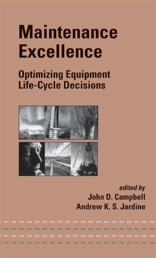
2. How long until you get 1% failures? Rearranging the equa-
tion for F (t) to solve for t
ln[1 Ϫ F (t)] ln(1 Ϫ 0.01)
tϭϪ ϭϪ ϭ 25,126 hr
λ 0.0000004
3. What would be the mean time to failure (MTTF)?
∞ ∞
MTTF ϭ Ύ
0
tf (t)dt ϭ Ύ tλe
0
Ϫλt
dt ϭ
1
λ
ϭ 2,500,000 hr
4. What would be the median time to failure (the time when
half the number will have failed?
F (T 50) ϭ 0.5 ϭ 1 Ϫ e ϪλT50
ln2 0.693
T 50 ϭ ϭ ϭ 1,732,868 hr
λ 0.0000004

273. 252 Chapter 9
This is the kind of information you can retrieve using the reli-
ability engineering principles in user-friendly software. Read
on to discover how.
9.6 REAL-LIFE CONSIDERATIONS:
THE DATA PROBLEM
Ironically, reliability management data can slip unnoticed
through your fingers as you relentlessly try to control mainte-
nance costs. Data management can prevent that from happen-
ing and provide critical information from past experience to
improve your current maintenance management process. It is
up to upper-level managers, though, to provide trained main-
tenance professionals with ample computer and technical
tools to collect, filter, and process data.
Without doubt, the first step in any forward-looking activ-
ity is to get good information. In fact, this is more important
than anything else. History proves that progress is built on
experience, but there are countless examples where ignoring
the past resulted in missed opportunities. Unfortunately,
many maintenance departments are guilty of this too.
Companies can be benchmarked against world-class best
practices by the extent to which their data effectively guides
their maintenance decisions and policies. Here are some ex-
amples of how you can make decisions using reliability data
management:
1. A maintenance planner notices that an in-service
component has failed three times within three
months. The superintendent uses this information to
estimate the failure numbers in the next quarter, to
make sure there will be enough people available to
fix them.
2. When ordering spare parts and scheduling mainte-
nance labor, determine how many gearboxes will be

274. Statistics and Economics of Maintenance 253
returned to the depot for overhaul for each failure
mode in the next year.
3. An effluent-treatment system must be shutdown and
overhauled whenever the contaminant level exceeds
a toxic limit for more than 60 seconds in a month.
Avoid these production interruptions by estimating
the level and frequency of preventive maintenance
needed.
4. After a design modification to eliminate a problem,
determine how many units must be tested, for how
long, to verify that the old failure mode has been elim-
inated, or significantly improved with 90% confi-
dence.
5. A haul truck fleet of transmissions is routinely over-
hauled at 12,000 hours, as stipulated by the manufac-
turer. A number of failures occur before the overhaul.
Find out how much the overhaul should be advanced
or retarded to reduce average operating costs.
6. The cost in lost production is 10 times more than for
preventive replacement of a worn component. From
this, determine the optimal replacement frequency.
7. You can find valuable information in the database to
help with maintenance decisions. For instance, if you
know the fluctuating values of iron and lead from
quarterly oil analysis of 35 haul truck transmissions,
and their failure times over the past three years, you
can determine the optimal preventive replacement
age (examined in Chapter 12).
Obviously, it is worth your while to obtain and record life
data at the system and, where warranted, component levels.
When tradespeople replace a component—say, a hydraulic
pump—they should indicate which specific pump failed. It
may be one of several identical pumps on a complex machine
that is critical to operations. They should also specify how it
failed, such as ‘‘leaking’’ or ‘‘insufficient pressure or volume.’’

275. 254 Chapter 9
Because we know how many hours equipment operates, we
can track the lifetime of individual critical components. That
information will then become a part of the company’s valuable
intellectual asset: the reliability database.
9.7 WEIBULL ANALYSIS
Weibull analysis supported by powerful software is formidable
in the hands of a trained analyst. Many examples and com-
ments are given in the practical guidebook The New Weibull
Handbook (2).
One of the distinct advantages of Weibull analysis is that
it can provide accurate failure analysis and forecasts with ex-
tremely small samples (2). Let’s look closely at the prime sta-
tistical failure investigation tool, the Weibull plot. Failure
data is plotted on Weibull probability paper but, fortunately,
modern software (3–6) provides a ‘‘virtual’’ version. The Wei-
bull plot uses x and y scales, transformed logarithmically so
that the Weibull CDF function:
F (t) ϭ 1 Ϫ eϪ (t/η) β
takes the form y ϭ βx ϩ Constant. By using Weibull probabil-
ity ‘‘paper,’’ you get a straight line when you plot failure data
that fits the Weibull distribution. What’s more, the slope of
the line will be the Weibull shape parameter β, and the charac-
teristic life η will be the time at which 63.2% of the failures
occurred.
9.7.1 Weibull Analysis Steps
Software makes Weibull analysis far more pleasant than it
used to be. Conceptually, the software:
• Groups the data in increasing order of time to failure,
as in Section 9.2.
• Obtains the median rank from tables for each time

276. Statistics and Economics of Maintenance 255
group (the median rank is explained in Section 9.7.3
and the median rank table for up to 12 samples is pro-
vided in Appendix 2)
• Plots on Weibull probability paper the median rank
versus failure time of each group of observations
For example, in the table in Figure 9-9, the April failures, will
have a median rank of 44.83% (Appendix 2), meaning that
roughly 44.83% of them occurred up to and including April.
The result is a plot such as Figure 9-9. You can see from the
graph that the shape parameter β is 1.97 and the characteris-
tic life η is 5.21. Furthermore, the mean life is 4.62 months
and the accuracy of how the data fits the Weibull distribution
is 99.08%.
Figure 9-9 Weibull plot.

277. 256 Chapter 9
9.7.2 Advantages
Much can be learned from the plot itself, even how the data
deviates from the straight line. For example:
• Whether and how closely the data follows the Weibull
distribution
• The type of failure (infant mortality, random, or
wearout)
• The component’s B n life (the time at which n% of a
population will have failed)
• Whether there may be competing failures (for exam-
ple, from fatigue and abrasion occurring simulta-
neously)
• Whether some other distribution, such as log normal,
is a better fit
• Whether there may have been predelivery shelf-life
degradation
• Whether there is an initial failure-free period that
needs to be accounted for
• Forecasts for failures at a given time or during a fu-
ture given period
• Whether there are batch or lot manufacturing defects
For more information about these deductions, see Ref. 2.
Surprisingly little data, as you will see, is required to
draw accurate and useful conclusions. Even with inadequate
data, engineers trained to read Weibull plots can learn a lot
from them. The horizontal scale is a measure of life or aging
such as start/stop cycles, mileage, operating time, takeoff, or
mission cycles. The vertical scale is the cumulative percentage
failed. The two defining parameters of the Weibull line are the
slope β and the characteristic life η.
The characteristic life η, also called the B 63.2 life, is the
age at which 63.2% of the units will have failed. Similarly,
where the Weibull line and the 10% CDF horizontal intersects
is the age at which 10% of the population fails, or the B 10 life.

278. Statistics and Economics of Maintenance 257
For more serious or catastrophic failures, the B 1, B 0.1 or B 0.01
lives are readily obtained from the Weibull plot.
The slope of the Weibull line, β, shows which failure class
is occurring. This could be infant mortality (decreasing hazard
function, β Ͻ 1), random (constant hazard function, β ϭ 1), or
wearout (increasing hazard function, β Ͼ 1). The B 63.2 life is
approximately equal to the mean-time-to-failure, MTTF.
(They are equal when β ϭ 1. That is when Weibull is equiva-
lent to the exponential distribution.) See Figure 9-10.
A significant advantage of the Weibull plot is that even
if you don’t immediately get a straight line (such as in Figure
9-9) when plotting the data, you can still learn something
quite useful. If the data points are curved downward (Figure
9-11, bottom), it could mean the time origin is not at zero. This
could imply that the component had degraded on the shelf, or
suffered extended burn-in time after it was made but before
delivery. On the other hand, it could show that it was physi-
cally impossible for the item to fail early on. Any of these rea-
sons could justify shifting the origin and replotting.
Alternatively, the concave downward curve could be say-
ing that the data really fit a log normal distribution. You can,
using software, quickly and conveniently test these hypothe-
ses, replot with a time-origin shift, or transform the scale for
log normal probability ‘‘paper.’’ Once you apply the appro-
Figure 9-10 Hazard function for burn-in, random, and wearout
failures.

279. 258 Chapter 9
priate origin-shift correction (adding or subtracting a value t 0
to each data point time), the resulting plot will be straight and
you will know a lot more about the failure process.
Further, if the plotted data forms a dogleg downward
(Figure 9-11, top), it could mean that something changed when
the failed part was manufactured. The first, steeper-sloped leg
reflects low time failures. The second, lower-sloped line indi-
cates failures from batches without the defect. When there are
dual failure modes like this, it’s known as a batch effect. When
there are many suspensions (parts that have been removed
for reasons besides failure, or parts that haven’t failed at the
end of the sampling period) it can be a clue that a batch prob-
lem exists. Failure serial numbers clustered closely along a
leg support the theory that there was some manufacturing
process change before the specific units were produced. Sched-
uled maintenance can also produce batch effects (2).
An upward-pointing dogleg bend (Figure 9-11, center) in-
dicates multiple failure modes. Investigate the failed parts. If
the different failures are plotted separately, treating the other
failure as a suspension, two straight lines should be observed.
This is the classic bi-Weibull, showing the need for a root cause
Figure 9-11 Various Weibull plotted data.

280. Statistics and Economics of Maintenance 259
failure analysis (RCFA) to eliminate, for example, an infant-
mortality problem. Several dogleg bends distinguish various
multiple failure modes (2).
When the Weibull plot forms a downward concave curve,
you may need to use an origin shift, t 0 , equivalent to using a
three-parameter Weibull (2):
F (t) ϭ 1 Ϫ eϪ(tϪt0/ηϪt0)β
There should be a physical explanation of why failures cannot
occur before t 0. For example, bearings, even in an infant-mor-
tality state, will continue to operate for some time before fail-
ing. Use a large sample size, at least 20 failures. If you know,
from earlier Weibulls, that the third parameter is appropriate,
you might use a smaller sample size, say, eight to ten (2).
For Weibull and other statistical modeling methods, the
data requirements are straightforward. Maintenance person-
nel should be able to collect it during routine activities. There
are three criteria for good data, stipulated by D. R. Cox (2):
1. The time origin must be clear.
2. The scale for measuring time must be agreed to.
3. The meaning of failure must be clear.
Although all modern CMMSs (Computerized Maintenance
Management Systems) and EAM (Enterprise Asset Manage-
ment) systems can provide this level of data collection, unfor-
tunately they have been mostly underused. To be fair, writing
out failure and repair details isn’t part of the tradesperson’s
job description. Many in the field don’t yet see that adding
meticulous information to the maintenance system makes or-
ganization assets function more reliably. Training in this area
could yield untapped benefits.
Although the technicians performing the work provide
the most useful information, collecting it is the responsibility
of everyone in maintenance. Data must be continually moni-

281. 260 Chapter 9
tored for both quality and relevance. Once the data flow is de-
veloped, it can be used in several areas, such as developing
preventive maintenance programs, predictive maintenance,
warranty administration, tracking vendor performance, and
improved decision making (7). As Weibull analysis and other
reliability methods become prevalent through advanced soft-
ware, data will improve. The result? Management and staff
will recognize the potential of good data to sharpen their com-
pany’s competitive edge.
9.7.3 Median Ranks
Suppose that five components fail at 67, 120, 130, 220, and
290 hours. To plot this data on Weibull probability paper, you
need the CDF’s corresponding estimates. You must estimate
the fraction that is failing before each of the failure ages. You
can’t simply say that the percentage failed at 120 hours is 40
(2/5), because that would imply that the cumulative probabil-
ity at 290 hours, a random variable, is 100%. This small sam-
ple size doesn’t justify such a definitive statement. Taken to
the absurd, from a sample size of 1 you certainly couldn’t con-
clude that the time of the single failure reflects 100% of total
failures. The most popular approach to estimating the Y-axis
plotting positions is the median rank. Obtain the CDF plotting
values from the median ranks table in Appendix 2, or from a
reasonable estimate of the median rank, Benard’s formula:
i Ϫ 0.3
Median rank ϭ
n Ϫ 0.4
where i ϭ chronological order of the component’s failure and
n ϭ sample size, 5 in this instance.
Determined by either method, this item’s cumulative fail-
ure probabilities are 0.13, 0.31, 0.5, 0.69, and 0.87, respec-
tively, for the first, second, third, fourth, and fifth ordered fail-
ure observations. When you use reliability software, you do
not have to look up the median ranks in tables or perform

282. Statistics and Economics of Maintenance 261
manual calculations. The program automatically calculates
and applies the median ranks to each observation.
9.7.4 Censored Data or Suspensions
It is an unavoidable data-analysis problem that, at the time
you are observing and analyzing, not all the units will have
failed. You know the age of the unfailed units and that they
are still working properly, but not when they will fail. Also,
some units may have been replaced preventively. In those
cases too, you don’t know when they would have failed. These
units are said to be suspended or right-censored. Left-censored
observations are failures whose starting times are unavail-
able. While not ideal, statistically you can still use censored
data, since you know that the units lasted at least this long.
Ignoring censored data would seriously underestimate the
item’s reliability.
Account for censored data by modifying the order num-
bers before plotting and determining the CDF values (from
Benard’s formula or from the median ranks table). Assuming
item 2 was removed without having failed, the order numbers
1, 2, 3, 4, and 5 in the previous section (9.7.3) would become:
1, 2.5, 3.75, and 5.625. The formula used to calculate these
modified orders is in Appendix 3. Consequently, the modified
median ranks would become those shown in Table 9-1. Now
Table 9-1 Modified Orders and Median Ranks for Samples with
Suspensions
Modified Median
Hours Event Order order rank
67 F 1 1 0.13
120 S 2 — —
130 F 3 2.5 0.41
220 F 4 3.75 0.64
290 F 5 5.625 0.99
F, failure; S, suspension (or censored observation).

283. 262 Chapter 9
you can plot the observations on Weibull probability paper
normally.
9.7.5 The Three-Parameter Weibull
For the reasons described in Section 9.7.2, including physical
considerations, the time of the observations may need to be
shifted for the Weibull data to plot to a straight line. By chang-
ing the origin, you activate another parameter in the Weibull
equation. To make the model work, you must estimate three
parameters rather than two. See Appendix 4 for the procedure
to estimate the third parameter, also called the location pa-
rameter, the guarantee life, or the minimum-life parameter
(8). A two-parameter Weibull model is a special case of the
more general three-parameter model, with the location pa-
rameter equal to zero.
9.7.6 The Five Parameter Bi-Weibull (9)
As shown in Figure 9-11, more than one behavior (of burn-in,
random, and wearout) can be reflected by your sample data.
The bi-Weibull model can represent two failure types, for
example, a stress (random) failure-rate phase followed by a
wearout phase; a random phase followed by another random
phase, at some higher failure rate; or a burn-in failure fol-
lowed by random failure. Six common failure patterns are il-
lustrated in Figure 9-12.
A limitation of the Weibull distribution is that it does not
cover patterns B and F (Figure 9-12), which often occur (9). A
bi-Weibull distribution is formed by combining two Weibull
distributions. The five-parameter Weibull, known as the Has-
tings bi-Weibull, is implemented in the RelCode (3) package.
Its hazard function form is:
βϪ1
h(t) ϭ λθ(λγ) θϪ1
ϩ
΂ ΃΂ ΃
β
η
tϪγ
η

284. Statistics and Economics of Maintenance 263
Figure 9-12 System failure rate patterns.
If γ ϭ θ ϭ 0, the Hastings bi-Weibull reduces to a Weibull dis-
tribution. The bi-Weibull distribution includes the Weibull as
a special case, but allows two failure phases, so patterns B and
F are now covered. Software (3) will fit the most appropriate of
the various models (two-parameter Weibull, three-parameter
Weibull, or five-parameter bi-Weibull) to the data. For a ran-
dom failure phase followed by a wearout phase, knowing the
onset of the wearout helps decide when to begin preventive
repair or replacement.
9.7.7 Confidence Intervals
You need to be confident that any actions you take based on
your statistical analysis and observed data modeling will be
successful. In Figure 9-9, we plotted failure observation times
of 48 failures over a period of 10 months against the CDF val-
ues estimated by the median rank. The median rank estimates
that 50% of the time the true percentage of failures lies above
or below it.
Similarly, you can estimate the CDF according to another

285. 264
Table 9-2 Cumulative Probability Distribution Including 95% and 5% Ranks
Month: Jan Feb Mar Apr May Jun Jul Aug Sep Oct
Failures: 2 5 7 8 7 6 5 4 3 1
Median rank: 3.47 13.84 28.31 44.83 54.30 71.70 82.02 90.30 96.49 98.55
95% rank: 9.51 23.19 39.57 56.60 70.41 81.43 89.85 95.81 99.23 99.89
5% rank: 0.75 7.05 18.57 33.43 47.52 60.43 71.93 81.94 90.49 93.95
Chapter 9

286. Statistics and Economics of Maintenance 265
Figure 9-13 Weibull plot showing 5% and 95% confidence limits.
set of tables, the 95% rank tables. This allows that 95% of the
time the percentage of failures will be below this value. The
same applies for a 5% rank, where 95% of the time the percent-
age will be above this value. Table 9-2 introduces rows for the
5% and 95% rank values into our original example. The 5%
and 95% rank tables are given in Appendix 5. Figure 9-13
shows the data of Table 9-2 on the Weibull plot.
From the Weibull plot of the median, between 95%, and
5% rank lines, you can conclude that the distribution function
at the end of May will have a value between 48% and 70%,
with a confidence of 90%. This means that, after 5 months, in
90% of the tests you conduct, between 48% and 70% of the
items will fail. Or that the reliability (which is 100% minus
the CDF value) of this type of item surviving 5 months is be-
tween 30% and 52%, 90% of the time.
The vertical distance between the 5% and 95% lines

287. 266 Chapter 9
represents a 90% confidence interval. By plotting all three
lines, you get a confidence interval showing that the cumu-
ulative probability of failure will assume a value in the in-
terval defined by the intersection of the age and the 5% and
95% lines, with 90% confidence. As a second example, an
item’s failure probability, up to and including June, is be-
tween 60% and 81%, 90% of the time. Or, knowing that
R(t) ϭ 1 Ϫ F(t), the item’s reliability that it will survive to
the end of 6 months is between 19% and 40%, with 90%
confidence. See Appendix 5 for another example of how this
methodology achieves a confidence interval for an item’s reli-
ability.
9.7.8 Goodness of Fit
You would, quite naturally, like to have a quantitative mea-
sure of how well your model fits the data. How good is the fit?
Goodness-of-fit testing provides the answer. Methods such as
least-squares or maximum-likelihood (described in Appendix
6) are used to fit an assumed distribution model to the data
and estimate the parameters of its distribution function. That
information, and the confidence intervals discussed in the pre-
vious section, will help you judge the validity of your model
choice (be it Weibull, log normal, negative exponential, or an-
other) and your estimation method. One of the methods com-
monly used is the Kolmogorov-Smirnov test described in Ap-
pendix 7.
9.8 ECONOMIC CONSIDERATIONS IN
PHYSICAL ASSET MANAGEMENT
Many asset management decisions, such as whether to replace
an expensive piece of equipment, require large investments of
money. The cost and benefits will continue for a number of
years. When an investment today influences future cash flow,
keep in mind that the money’s value now depends on when it

288. Statistics and Economics of Maintenance 267
is due. For example, $1000 received in the future is worth less
than $1000 received today.
To compare alternative investments, convert the future
dollar costs and benefits to their present-day value. In one nu-
merical index, you can summarize the current value of cash
flow streams, and rank alternative investments in order of
preference (7).
9.8.1 Aspects of Discounting for Capital
Equipment Replacement Analysis
If you invest $1000 in a bank account, at an annual interest
rate of 10%, after 1 year you will have $1100. If you leave the
money in the bank for another year, and the 10% interest rate
remains, it will grow to $1210. Discounting uses the same fa-
miliar calculation, but in reverse. For example, if you know
that in 2 years you will have a maintenance bill of $1210, you
can determine the value today of that future cash flow. If the
interest rate for discounting is 10%, the current value will be
$1000. Details of the calculation are provided in Appendix 8,
‘‘Present Value.’’
The key to discounting is knowing the right interest rate
to use in your calculations. Most organizations have clearly
stated rates, taking into account the time value of money in
capital equipment replacement decisions (7). Rates used in-
clude:
• Rate of return on new investments
• Weighted average of market yields on debt and equity
• Cost of additional borrowing
• Rate that keeps the market price of a common stock
from falling
• Spread between the prime rate and inflation
The examples in Chapter 11, ‘‘Optimizing Maintenance
and Replacement Decisions,’’ specify the interest rate to use
and explain the calculation method.

289. 268 Chapter 9
Another economic calculation is to convert the present
value of a replacement policy to an equivalent annual cost
(EAC). This shows the constant value of the cash flow year to
year. Some years produce high cash flow—from purchasing
new assets, for instance. There are also low-yielding years,
such as when maintenance costs are covered by warranty. The
EAC smoothes them out into an ‘‘average’’ value year to year
for the actual cash flows. See Appendix (9) for a detailed EAC
description.
REFERENCES
1. Ernst G. Frankel. Systems Reliability and Risk Analysis. 2nd
ed. Norwell, MA: Kluwer Academic, 1983.
2. Robert B. Abernethy. The New Weibull Handbook. 2nd ed.
Houston: Gulf Publishing, 1996.
3. Oliver Interactive Inc.: www.oliver-group.com.
4. ReliaSoft: www.weibull.com/home.htm.
5. M-Tech Consulting Engineers: http://www.m-tech.co.za.
6. WinSmith for Windows, Fulton Findings: http://www/weibull
news.com.
7. Andrew K.S. Jardine. Optimizing Equipment Maintenance and
Replacement Decisions, course notes. Department of Mechani-
cal and Industrial Engineering, University of Toronto.
8. K.C. Kapur, L.R. Lamberson. Reliability in Engineering De-
sign. New York: Wiley, 1977.
9. N.A.J. Hastings. RelCode for Windows User’s Manual.
BIBLIOGRAPHY
Fabrycky, W.J., Thuesen, Gerald J. Engineering Economy, 9th ed.
Englewood Cliffs, NJ: Prentice Hall, 2001.
Park, C.S., Pelot, R., Porteous, K.C., Zuo, M.J. Contemporary Engi-
neering Economics, 2nd Canadian Edition. Toronto: Addison
Wesley Longman, 2000.
RelCode Users’ Manual. Albany Interactive, Samford Valley,
Queensland, Australia 4520. albany.interactive@bigpond.com

290. 10
Maintenance Optimization Models
Maintenance optimization is all about getting the best result
possible, given one or more assumptions. In this chapter, we
introduce the concept of optimization through a well under-
stood traveling problem—identifying the best mode of travel,
depending on different requirements. We also examine the im-
portance of building mathematical models of maintenance de-
cision problems to help arrive at the best decision.
We look at key maintenance decision areas: component
replacement, capital-equipment replacement, inspection pro-
cedures, and resource requirements. We use optimization
models to find the best possible solution for several problem
situations.
Finally, you will learn about the role that artificial intelli-
gence plays in optimization of maintenance decisions.
269

291. 270 Chapter 10
10.1 WHAT IS OPTIMIZATION ALL ABOUT?
Optimal means the most desirable outcome possible under re-
stricted circumstances. For example, following an RCM study,
you could conduct condition-monitoring maintenance tactics
and/or time-based maintenance and/or time-based discard for
specific parts of a machine or system.
In this chapter, we introduce maintenance decision optimi-
zation. In the following two chapters, we discuss detailed mod-
els for asset maintenance and replacement decision making.
To understand the concept of optimization, consider this
travel routing problem: you have to take an airplane trip, with
three stops, before returning home to Chicago. First destina-
tion is London, then Moscow, and finally Hawaii.
Before purchasing a ticket, you would weigh a number of
options, including airlines, fares, and schedules. You’d make
your decision based on such factors as economy, speed, safety,
and extras.
• If economy is most important, you’d choose the airline
with the cheapest ticket. That would be the optimal
solution.
• If speed is your top priority, you’d consider only the
schedules and disregard the other criteria.
• If you wanted to optimize safety, you’d avoid airlines
with a dubious safety record and pick only a well-
regarded carrier.
• If you wanted a free hotel room (an ‘‘extra’’) for three
nights in Hawaii, you’d opt for the airline that would
provide that benefit.
The above illustrates the concept of optimization. When you
optimize in one area—economy, for example—then you al-
most always get a less desirable (suboptimal) result in one or
more of the other criteria.
Sometimes you have to accept a tradeoff between two cri-
teria. For example, although speed may be most important to

292. Maintenance Optimization Methods 271
you, the cost of traveling on the fastest schedule might be un-
acceptable. The solution is somewhere in the middle: opting
for an acceptable cost (but not the very lowest) and speed (but
not the very fastest).
In any optimization situation, including maintenance de-
cision optimization, you should:
• Think about optimization when making maintenance
decisions.
• Consider what maintenance decision you want to opti-
mize.
• Explore how you can do this.
10.2 THINKING OPTIMIZATION
Thinking about optimization means considering tradeoffs—
the pros and cons. Optimization always has to do with getting
the best result where it counts most, while consciously ac-
cepting less than that elsewhere.
A Customer Service Manager was asked by the VP of
Marketing what he thought his main mission was. His an-
swer: to get every order for every customer delivered without
fail on the day the customer specified, 100% of the time. To
achieve this goal, the inventory of ready-to-ship goods would
have to include every color, size, and style in sufficient quanti-
ties to ensure that no matter what was called for, it could be
shipped. In spite of unusually big orders, a large number of
customers randomly wanting the same thing at the same time,
or machinery failure, the manager would have to deliver. His
inventory would have had an unacceptably high cost.
The manager failed to realize that a delivery performance
just slightly less, say 95%, would be better. In fact, it would
be a profit-optimization strategy, the best tradeoff between the
cost of inventory and an acceptable and competitive customer-
satisfaction level.

293. 272 Chapter 10
10.3 WHAT TO OPTIMIZE
Just as in other areas, you can optimize in maintenance for
different criteria, including cost, availability, safety, and profit.
Lowest-costs optimization is often the maintenance
goal. The cost of the component or asset, labor, lost production,
and perhaps even customer dissatisfaction from delayed deliv-
eries are all considered. Where equipment or component wear-
out is a factor, the lowest possible cost is usually achieved by
replacing machine parts late enough to get good service out
of them but early enough for an acceptable rate of on-the-job
failures (to attain a zero rate, you’d probably have to replace
parts every day).
Availability can be another optimization goal: getting
the right balance between taking equipment out of service for
preventive maintenance and suffering outages due to break-
downs. If safety is most important, you might optimize for the
safest possible solution but with an acceptable impact on cost.
If you optimize for profit, you would take into account not only
cost but the effect on revenues through greater customer satis-
faction (better profits) or delayed deliveries (lower profits).
10.4 HOW TO OPTIMIZE
One of the main tools in the scientific approach to manage-
ment decision making is building an evaluative model, usually
mathematical, to assess a variety of alternative decisions. Any
model is simply a representation of the system under study.
When applying quantitative techniques to management prob-
lems, we frequently use a symbolic model. The system’s rela-
tionships are represented by symbols and properties described
by mathematical equations.
To understand this model-building approach, examine
the following maintenance stores problem. Although simpli-
fied, it illustrates two important aspects of model use: con-

294. Maintenance Optimization Methods 273
Figure 10-1 An inventory problem.
structing a model of the problem being studied and its solu-
tion.
10.4.1 A Stores Problem
A stores controller wants to know how much to order each time
the stock level of an item reaches zero. The system is illus-
trated in Figure 10-1. The conflict here is that the more items
ordered at any time, the more ordering costs will decrease but
holding costs increase, since more stock is kept on hand. These
conflicting features are illustrated in Figure 10-2. The stores
controller wants to determine which order quantity will mini-
mize the total cost. This total cost can be plotted, as shown on
Figure 10-2, and used to solve the problem.
A much more rapid solution, however, is to construct a
mathematical model of the decision situation. The following
parameters can be defined:
D ϭ Total annual demand
Q ϭ Order quantity
C o ϭ Ordering cost per order
C h ϭ Stockholding cost per item per year
Total cost per year of ϭ Ordering cost per year ϩ
ordering and holding stock Stockholding cost per year

295. 274 Chapter 10
Figure 10-2 Economic order quantity.
Now
Ordering cost per year ϭ Number of orders placed
per year ϫ Ordering cost
per order
D
ϭ Co
Q
Stockholding cost per year ϭ Average number of items
in stock per year (assum-
ing linear decrease of
stock) ϫ Stockholding cost
per item
Q
ϭ Ch
2
Therefore, the total cost per year, which is a function of the
order quantity and denoted C(Q), is

296. Maintenance Optimization Methods 275
D Q
C(Q) ϭ Co ϩ Ch (1)
Q 2
Equation (1) is a mathematical model of the problem relating
order quantity Q to total cost C(Q).
The stores controller wants to know the number of items
to order to minimize the total cost, i.e., the right-hand side of
Equation (1). The answer is obtained by differentiating the
equation with respect to Q, the order quantity, and equating
the answer to zero as follows:
dC(Q) D C
ϭ Ϫ 2 Co ϩ h ϭ 0
dQ Q 2
Therefore:
D C
Co ϭ h
Q2 2
√
2DC o
Qϭ (2)
Ch
Since the values of D, C o , and C h are known, substituting them
into Equation (2) optimizes the value of the order quantity Q.
Strictly check that the value of Q obtained from Equation 2
is a minimum and not a maximum. You can ensure that this
is the case by taking the second derivative of C(Q) and noting
the positive result. In fact, the order quantity equalizes the
holding and ordering costs per year.
Example: Let D ϭ 1000 items, C o ϭ $5, C h ϭ $0.25:
√
2 ϫ 1000 ϫ 5
Qϭ ϭ 200 items
0.25
Each time the stock level reaches zero, the stores controller
should order 200 items to minimize the total cost per year of
holding and ordering stock.

297. 276 Chapter 10
Note that various assumptions have been made in the in-
ventory model presented, which may not be realistic. For ex-
ample, no consideration has been given to quantity discounts,
the possible lead time between placing an order and its re-
ceipt, and the fact that demand may not be linear or known for
certain. The purpose of the above model is simply to illustrate
constructing a model and attaining a solution for a particular
problem. There is abundant literature about stock-control
problems without many of these limitations. If you are inter-
ested in stock-control aspects of maintenance stores, see Nah-
mias (1).
It’s clear from the above inventory control example that
we need the right kind of data, properly organized. Most orga-
nizations have a Computerized Maintenance Management
System (CMMS) or an Enterprise Asset Management (EAM)
system. The vast amount of data they store makes optimiza-
tion analyses possible.
Instead of building mathematical models of maintenance
decision problems, software is available to help you make op-
timal maintenance decisions. This is covered in Chapters 11
and 12.
10.5 KEY MAINTENANCE MANAGEMENT
DECISION AREAS
There are four key decision areas that maintenance managers
must address to optimize their organization’s human and
physical resources. These areas are depicted in Figure 10-3.
The first column deals with component replacement, the sec-
ond with establishing the economic life of capital equipment,
the third with inspection decisions, including condition moni-
toring. The final column addresses decisions concerning re-
sources required for maintenance and their location. To build
strong maintenance optimization, you need an appropriate
source, or sources, of data. The foundations for this, as shown
in Figure 10-3, are the CMMS and the EAM system.

298. Maintenance Optimization Methods 277
Figure 10-3 Maintenance decision optimization.

299. 278 Chapter 10
In Chapters 11 and 12 we discuss optimization of key
maintenance decisions in component replacement, capital
equipment replacement, and inspection procedures (columns
1, 2, and 3 of the framework illustrated in Figure 10-3). The
framework’s foundation, or database, is addressed in detail in
Chapter 4. In this chapter, we focus on column 4, resource re-
quirements, and comment briefly on the role of artificial intel-
ligence in maintenance optimization.
10.5.1 Resource Requirements
When it comes to maintenance resource requirements, you
must decide what resources there should be, where they
should be located, who should own them, and how they should
be used.
If sufficient resources aren’t available, your maintenance
customers will be dissatisfied. Having too many resources,
though, isn’t economical. Your challenge is to balance spend-
ing on maintenance resources such as equipment, spares, and
staff with an appropriate return for that investment.
10.5.2 Role of Queuing Theory to Establish
Resource Requirements
The branch of mathematics known as queuing theory, or
waiting-line theory, is valuable in situations where bottle-
necks can occur. You can explore the consequences of alterna-
tive resource levels to identify the best option. Figure 10-4 il-
lustrates the benefit of using queuing theory to establish the
optimal number of lathes for a workshop. In this example the
objective is to ensure that the total cost of owning and op-
erating the lathes and tying up jobs in the workshop is mini-
mized. For a model of this decision process, see Appendix 10.
10.5.3 Optimizing Maintenance Schedules
In deciding maintenance resource requirements, you must
also consider how to use resources efficiently. An important

300. Maintenance Optimization Methods 279
Figure 10-4 Optimal number of machines in a workshop.
consideration is scheduling jobs through a workshop. If there
is restricted workshop capacity and jobs cannot be contracted
out, you must decide which job should be done first when a
workshop machine becomes available.
Sriskandarajah et al. (2) present a unique and highly
challenging maintenance overhaul scheduling problem at the
Hong Kong Mass Transit Railway Corporation (MTRC). In
this case, preventive maintenance keeps trains in a specified
condition, taking into account both the maintenance cost and
equipment-failure consequences. Since maintenance tasks
done either ‘‘too early’’ or ‘‘too late’’ can be costly, how mainte-
nance activities were scheduled was important.
Smart scheduling reduces the overall maintenance bud-
get. In establishing a schedule, it’s essential to acknowledge
constraints, such as the number of equipment/machines that

301. 280 Chapter 10
can be maintained simultaneously, as well as economic, reli-
ability, and technological concerns. Most scheduling problems
are a combination of factors. Because of this complexity, a heu-
ristic technique known as genetic algorithms (GAs) was used
in this case to arrive at the global optimum.
The performance of the algorithm compared well with
manual schedules established by the Hong Kong MTRC. For
example, total costs were reduced by about 25%. The study
supports the view that genetic algorithms can provide good
solutions to difficult maintenance scheduling problems.
10.5.4 Optimal Use of Contractors
(Alternative Service Delivery Providers)
The above decision process assumed that all the maintenance
work had to be done within the railway company’s own main-
tenance facility. If you can contract out the maintenance
tasks, you must decide, for instance, whether to contract out
all, some, only during peak demand periods, or none of them.
The conflicts of making such decisions are illustrated in Fig-
ure 10-5.
If your organization doesn’t have any maintenance re-
sources, you will need to contract out all the work. The only
cost will be paying for the alternative delivery service. If your
organization has a maintenance division, though, there will
be two cost components. One is a fixed cost for the facility,
shown in Figure 10-5 to increase linearly as the facility size
expands. The second cost is variable, increasing as more work
is handled internally but leveling off when there is overca-
pacity.
The optimal decision is a balance between internal re-
sources and contracting out. Of course, this isn’t always the
best solution. You have to assess the demand pattern, and
both internal and external maintenance costs. If it is cheaper
not to have an internal maintenance facility, the optimal solu-
tion would be to contract out all the maintenance work. Alter-
natively, the optimal solution could be to gear up your own

302. Maintenance Optimization Methods 281
Figure 10-5 Optimal contracting-out decision.
organization to do all the work internally. See Appendix 11
for a model of this decision process.
10.5.5 Role of Simulation in
Maintenance Optimization
Common maintenance management concerns about resources
include:
• How large should the maintenance crews be?
• What mix of machines should there be in a workshop?
• What rules should be used to schedule work through
the workshop?
• What skill sets should we have in the maintenance
teams?
Some of these questions can be answered by using a mathe-
matical model. For complex cases, though, a simulation model

303. 282 Chapter 10
of the decision situation is often built. You can use the simula-
tion to evaluate a variety of alternatives, then choose the best.
Many simulation software packages are available that require
minimal programming.
Many resource decisions are complex. Take, for example,
a situation where equipment in a petrochemical plant requires
attention. If the maintenance crew is limited by size or at-
tending to other tasks, the new job may be delayed while an-
other emergency crew is called in. Of course, if there had been
a large crew in place initially, this wouldn’t have occurred.
Since there can be many competing demands on the mainte-
nance crew, it’s difficult to establish the best crew size.
This is where simulation is valuable. Figure 10-6 illus-
trates a case in which simulation was used to establish the
Figure 10-6 Maintenance crew size simulation.

304. Maintenance Optimization Methods 283
optimal maintenance crew size and shift pattern in a petro-
chemical plant. For illustration purposes, statistics are pro-
vided for the failure pattern of select machines, along with
repair-time information. The study was undertaken to in-
crease the plant’s output. The initial plan was to add a fourth
finishing line, to reduce the bottleneck at the large mixing
tank (TK18XB), just before the finishing lines. The
throughput data, though, showed that once a machine failed,
there was often a long wait until the maintenance crew ar-
rived. Rather than construct another finishing line, it was de-
cided to increase maintenance resources. By using simulation,
the throughput from the plant was significantly increased
with little additional cost. Increasing crew size was a much
cheaper alternative and achieved the required increased
throughput.
10.6 ROLE OF ARTIFICIAL INTELLIGENCE
IN MAINTENANCE OPTIMIZATION:
EXPERT SYSTEMS AND NEURAL
NETWORKS
Collecting data for maintenance decision making is the rela-
tively easy part. There are many hardware and software prod-
ucts with impressive accuracy, capacity, and computer inter-
faces on the market. The result is oceans of data. However,
analyzing the data is more difficult, because human experts
are required to interpret it. Two technological solutions are in
varying evolutionary states: expert systems and neural net-
works.
10.6.1 Expert Systems
Table 10-1 shows the kind of experience and engineering
know-how you will find in expert system knowledge bases.
It presents the likelihood that a particular problem is re-
lated to the pattern of vibration irregularities by frequency
order.

305. 284 Chapter 10
Table 10-1 An Example of an Expert System Knowledge Base
Probabilities (%)
Fault 1x rpm 2x rpm Ͼ2x Ͼ
Ͼ2x Other Ͻ1x
Shaft imbalance 90 5 5
Shaft bent 90 5 5
Lost rotor vanes 90 5 5
Case distortion 60 20 10 10
Foundation distortion 40 30 10 20
Bearing damage 40 20 20
Gear damage 20 60 20
Bearing casing loose 30 10 90
Bearing liner loose 10 90
Bearing eccentricity 40 60
Casing structural resonance 70 10 10
Coupling damage 20 30 10 80 20
Rotor resonance 100
Rotor looseness 10 10 10 10 40
Shaft misalignment 30 60 10
Expert systems are a branch of artificial intelligence.
They can be used to process and interpret large numbers of
data, including trends, ratios, and other combinations of sig-
nals. Figure 10-7 depicts a rule that is part of an expert system
knowledge base on oil analysis.
Expert systems consist of rules, possibly thousands, such
as those in Figure 10-7, that ‘‘fire’’ in sequence to arrive at a
set of final recommendations. When all the conditions in the
IF part of the rule are true, the rule fires. Each statement,
called a choice, in the THEN and ELSE part of a rule is
weighted (3). The same choices can appear in many rules.
Their weights are totaled and divided by the number of times
they appear in rules that have fired. A choice will appear in
the set of final recommendations if its average weight exceeds
some predefined limit, say 8/10. A fuzzy expert system is an
expert system that uses a collection of fuzzy membership func-
tions and rules, instead of Boolean logic, to reason about data
(described in Appendix 12).

306. Maintenance Optimization Methods 285
Figure 10-7 An oil-analysis expert system rule.
10.6.2 Neural Networks
A disadvantage of expert systems is their dependence on hu-
man knowledge. Programming the expert system with human
experience can be time-consuming and error-prone. Another
approach is to use neural networks, the other main branch
of artificial intelligence. Unlike expert systems, they do not
require that human knowledge be programmed into them, be-
cause they observe and learn on their own during a training
period.
Each of the nodes in Figure 10-8 is called a neuron. This
type of neural network is known as a multilayer perceptron
(MLP). The neurons of an MLP are arranged in layers. The
bottom layer is the input layer. The top one is the output layer.
There can be any number of middle or hidden layers. The lines
connecting the nodes are known as synaptic links, whose val-
ues or weightings change as the neural net is trained.

307. 286 Chapter 10
Figure 10-8 A neural network.
Figure 10-8 represents a three-layer neural network, pro-
viding XOR (the Boolean ‘‘exclusive or’’) functionality. After a
suitable training period the values of the synaptic links are
as shown. To get an answer, first compute the sum of inputs
to the hidden layer neuron h: s ϭ (1 ϫ 7.1) ϩ (1 ϫ Ϫ2.76) ϩ
(0 ϫ 7.1) ϭ 4.34. Then apply an activation function v ϭ 1/(1
ϩ e Ϫs) to compute the activation value, v ϭ 1/(1 ϩ e Ϫ4.34) ϭ
0.98%. The output neuron is computed similarly: s ϭ (1 ϫ
Ϫ4.95) ϩ (0 ϫ Ϫ4.95) ϩ (0.98% ϫ 10.9) ϩ (1 ϫ Ϫ3.29) ϭ 2.52
and v ϭ 0.926. Of course, 0.91 is not quite 1 but for this exam-
ple, is close enough. Appendix 13 shows how this particular
neural net is trained. You will find more practical information
on neural networks in Ref. 4.
A Condition Maintenance Fault Diagnosis (CMFD) sys-
tem can use an MLP classifier to determine the state of a plant
from a measurement pattern. The classifier chooses a class
from among a number of predefined classes (e.g., Normal,
Fault A, Fault B, etc). Each potential condition is represented
by an output neuron.
Training neural networks is like ‘‘curve fitting.’’ Think of

308. Maintenance Optimization Methods 287
it as a form of nonlinear regression (4). One limitation is that
you may need an astronomical number of training cycles for
problems with many inputs, such as those related to condition-
based maintenance. Nonetheless, active research is reporting
new successful applications (5). Among them, neural nets
have become popular in cameras and cars, in which the auto-
matic transmission learns your driving style during the first
few hundred miles.
REFERENCES
1. S. Nahmias. Production and Operations Analysis. 3rd ed. Irwin/
McGraw-Hill, 1997.
2. C. Sriskandarajah, A. K. S. Jardine, C. K. Chan. Maintenance
Scheduling of Rolling Stock Using a Genetic Algorithm. Journal
of the Operational Research Society 1998; 49:1130–1145.
3. www.exsys.com.
4. Donald R. Tveter. Manual to the pro version of Backprop Algo-
rithm software. http://www.dontveter.com/bpr/bptutinps.zip
and http:/ /www.dontveter.com/bpr/public2.html.
5. M. H. Jones and D. G. Sleeman, eds. Condition Monitoring ’99.
Coxmoor Publishing, 1999.

310. 11
Optimizing Maintenance and
Replacement Decisions
In this chapter, we explore the various strategies and tools
you need to make the best maintenance and replacement deci-
sions. In particular, you need to know the optimal replacement
time for critical system components (also known as line-
replaceable units, or LRUs), and capital equipment.
At the LRU level, we examine age- and block replacement
strategies. You’ll learn how RelCode software can help you op-
timize LRU maintenance decisions to keep costs under control
and increase equipment availability.
With capital equipment, it’s critical to establish economic
viability. We examine how to do this in two operating environ-
ments:
• Constant use, year by year
• Declining use, year by year (older equipment is used less)
289

311. 290 Chapter 11
In this chapter, you’ll discover how to extend the life of
capital equipment through a major repair or rebuild, and
when that is more economical than replacing it with new
equipment. The optimal decision is the one that minimizes the
long-run Equivalent Annual Cost (EAC), the life-cycle cost of
owning, using, and disposing of the asset. Our study of capital-
equipment replacement includes a description of AGE/CON
and PERDEC software, which simplify the job of managing
assets.
Finally, we address the importance of inspection fre-
quency, including a case study for a fleet of buses subject to
A, B, C, and D inspection levels.
11.1 INTRODUCTION: ENHANCING
RELIABILITY THROUGH
PREVENTIVE REPLACEMENT
Generally, preventing a maintenance problem is always pre-
ferred to fixing it after the fact. You’ll increase your equipment
reliability by learning to replace critical components at the op-
timal time, before a breakdown occurs. When is the best time?
That depends on your overall objective. Do you most want to
minimize costs or maximize availability? Sometimes the best
preventive replacement time accomplishes both objectives,
but not necessarily.
Before you start, you need to obtain and analyze data to
identify the best preventive replacement time. Later in this
section, we present some maintenance policy models of fixed
interval and age-based replacements to help you do that.
For preventive replacement to work, these two conditions
must first be present:
1. If cost is most important, the total cost of a replace-
ment must be greater after failure than before. If re-
ducing total downtime is most essential, the total
downtime of a failure replacement must be greater

312. Maintenance and Replacement Decisions 291
than a preventive replacement. In practice, this usu-
ally happens.
2. The risk of a component failing must increase as it
ages. How can you know? Check that the Weibull
shape parameter associated with the component’s
failure times is greater than 1. It is often assumed
that this condition is met, but be sure that is in fact
the case. See Chapter 9 for a detailed description of
Weibull analysis.
11.1.1 Block Replacement Policy
The block replacement policy is sometimes called the group or
constant interval policy, since preventive replacement occurs
at fixed times and failure replacements whenever necessary.
The policy is illustrated in Figure 11-1. Cp is the total cost of
a preventive replacement, Cf is the total cost of a failure re-
placement, and tp is the interval between preventive replace-
ments.
You can see that for the first cycle of tp, there isn’t a fail-
ure, while there are two in the second cycle and none in the
third and fourth. As the interval between preventive replace-
ments decreases, there will be fewer failures in between. You
want to obtain the best balance between the investment in
preventive replacements and the economic consequences of
failure replacements. This conflict is illustrated in Figure
11-2. C(tp) is the total cost per week of preventive replace-
ments occurring at intervals of length tp, with failure replace-
Figure 11-1 Constant-interval replacement policy.

313. 292 Chapter 11
Figure 11-2 Constant-interval policy: optimal replacement time.
ments occurring whenever necessary. See Appendix 14 for the
total cost curve equation.
The following problem is solved using RelCode software
(1), incorporating both the cost model and Weibull analysis to
establish the best preventive replacement interval.
11.1.1.1 Problem
A bearing has failed in the blower used in diesel engines. The
failure has been established according to a Weibull distribu-
tion, with a mean life of 10,000 km and a standard deviation
of 4500 km. The bearing failure is expensive, costing 10 times
as much to replace than if it had been done as a preventive
measure. Determine:
• The optimal preventive replacement interval (or block
policy) to minimize total cost per kilometer
• The expected cost saving of the optimal policy over a
run-to-failure replacement policy

314. Maintenance and Replacement Decisions 293
Figure 11-3 RelCode output: block replacement.
• Given that the cost of a failure is $2000, the cost per
km of the optimal policy
11.1.1.2 Result
Figure 11-3 shows a screen capture from RelCode. You can see
that the optimal preventive replacement time is 4140 kilome-
ters (4139.13 in the chart). The figure also provides valuable
additional information. For example:
• The cost per kilometer of the best policy is $0.0843/km
• The cost saving compared to a run-to-failure policy is
$0.1035/km (55.11%)
11.1.2 Age-Based Replacement Policy
In the age-based policy, the preventive replacement time de-
pends on the component’s age—if a failure replacement oc-
curs, the component’s time clock is reset to zero. In the block

315. 294 Chapter 11
Figure 11-4 Age-based replacement policy.
replacement policy, however, preventive replacements occur
at fixed intervals regardless of the operating component’s age.
In this case, the component is replaced only when it reaches
the specified age.
Figure 11-4 illustrates the age-based policy. Cp and Cf
represent the block replacement policy, and tp represents the
component age when preventive replacement occurs. You can
see that there aren’t any failures in the first cycle, which is
tp. After the first preventive replacement, the component must
have failed before reaching its next planned preventive re-
placement age. After the first failure replacement, the clock
is set to zero and the next preventive replacement scheduled.
However, before it’s reached, the component is again replaced
due to failure. After this second failure replacement, the com-
ponent survives to the planned preventive replacement age of
tp. Similarly, the next replacement cycle shows that the compo-
nent made it to its planned preventive age.
The conflicting cost consequences are identical to those
in Figure 11-2, except that the x-axis measures the actual age
(or utilization) of the item, rather than a fixed time interval.
See Appendix 15 for the mathematical model depicting this
preventive replacement policy.
The following problem is solved using RelCode software,
which incorporates the cost model, to establish the best pre-
ventive replacement age.
11.1.2.1 Problem
A sugar-refinery centrifuge is a complex machine composed of
many parts that can fail suddenly. It’s decided that the plow-

316. Maintenance and Replacement Decisions 295
setting blade needs preventive replacement. Based on the age-
based policy, replacements are needed when the setting blade
reaches a specified age. Otherwise, a costlier replacement will
be needed when the part fails. Consider the optimal policy to
minimize the total cost per hour associated with preventive
and failure replacements.
To solve the problem, you have the following data:
• The labor and material cost of a preventive or failure
replacement is $2000.
• The value of production losses is $1000 for a preven-
tive replacement and $7000 for a failure replacement.
• The failure distribution of the setting blade can be de-
scribed adequately by a Weibull distribution with a
mean life of 152 hours and a standard deviation of 30
hours.
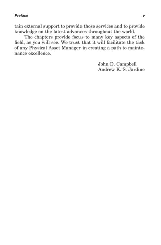
11.1.2.2 Result
Figure 11-5 shows a screen capture from RelCode. As you can
see, the optimal preventive replacement age is 112 hours
(111.77 hours in the figure), and there’s additional key infor-
mation that you can use. For example, the preventive replace-
ment policy costs 45.13% of a run-to-failure policy [(59.19 Ϫ
32.48)/59.1] ϫ 100, making the benefits very clear. Also, the
total cost curve is fairly flat in the 90 to 125 hours region, pro-
viding a flexible planning schedule for preventive replace-
ments.
11.1.3 When to Use Block Replacement
On the face of it, age replacement seems to be the only sensible
choice. Why replace a recently installed component that is still
working properly? In age replacement, the component always re-
mains in service until its scheduled preventive replacement age.
To implement an age-based replacement policy, though,
you must keep an ongoing record of the component’s current
age and change the planned replacement time if it fails.
Clearly, the cost of this is justified for expensive components,

317. 296 Chapter 11
Figure 11-5 RelCode output: age-based replacement.
but for an inexpensive one the easily implemented block re-
placement policy is often more cost-efficient.
11.1.4 Safety Constraints
With both block and age replacement, the objective is to estab-
lish the best time to preventively replace a component, to min-
imize the total cost of preventive and failure replacements. If
you want to ensure that the failure probability doesn’t exceed
a particular value—say, 5%—without cost considerations be-
ing formally taken into account, you can determine when to
schedule a preventive replacement from the cumulative fail-
ure distribution. This is illustrated in Figure 11-6, in which
you can see that the preventive replacement should be
planned once the item is at 4000 km.
Alternatively, you can preventively replace a critical com-
ponent so that the risk, or hazard, doesn’t exceed a specified

318. Maintenance and Replacement Decisions 297
Figure 11-6 Optimal preventive replacement age: risk-based
maintenance.
value, such as 5 ϫ 10Ϫ5 failures per km. In this case, you need to
use the hazard plot to identify the preventive replacement age.
This is illustrated in Figure 11-7, which shows that the compo-
nent’s appropriate preventive replacement age is 4500 km.
11.1.5 Minimizing Cost and Maximizing
Availability
In both block and age replacement, the objective is minimizing
cost. Maximizing availability simply requires replacing the to-
tal costs of preventive and failure replacement in the models
with their total downtime. Minimizing total downtime is then
equivalent to maximizing availability. In Appendix 16, you’ll
find total downtime-minimization models for both block and
age replacement.

319. 298 Chapter 11
Figure 11-7 Optimal preventive replacement age: hazard limit.
11.2 DEALING WITH REPAIRABLE
SYSTEMS
Rather than completely replace a failed unit, you may be able
to get it operating with minor corrective action. This is what’s
known as a minimal repair. It’s assumed that the unit’s over-
all hazard rate hasn’t been changed, that the maintenance fix
has simply made it operational again, and that the previous
hazard level has remained the same. This is illustrated in Fig-
ure 11-8, where h(t) is the component’s hazard rate at age t.
On the other hand, you could decide to take significant
maintenance action when an item fails. This is called a gen-
eral repair in maintenance and is illustrated in Figure 11-9.
You can see that a general repair reduces the unit’s hazard
rate, but not to zero, which would be the case if you completely
renewed it. Taking into account the costs of minimal repair (a

320. Maintenance and Replacement Decisions 299
Figure 11-8 Minimal repair.
minor fix), general repair (such as an overhaul), and a com-
plete renewal, you want to know the best maintenance action
when a unit fails.
This is an area that is not well developed, although prog-
ress is being made. One approach is illustrated in Figure
11-10. Virtual age, just after the last repair, is measured on
the x-axis and length of operating time (run time) since last
repair is measured on the y-axis, at the top of the figure. The
Figure 11-9 Minimal and general repair.

321. 300 Chapter 11
Figure 11-10 Repairable system optimization.
optimal policy for this system is explained through the differ-
ent regions shown in the figure.
When a failure occurs, if the repair cost—shown on the
y-axis in the bottom of the figure—is less than a constant
value C0, the maintenance is minimal repair. Otherwise, it is
a general repair, provided the cost doesn’t exceed the lower
boundary. If it does exceed the lower boundary, you must re-
place the system. You should preventively replace the system
whenever the length of operating time (run time) reaches the
upper boundary. Otherwise, the system is in the safe op-
erating region (2).
In Figure 11-10, you can see that at the start the unit
was of virtual age V0. At first failure time (X1), the cost was
C1, resulting in a general repair and the equipment’s virtual
age being V1. At failure time X2, the repair cost was C2 and,

322. Maintenance and Replacement Decisions 301
again, there is a general repair resulting in the unit’s virtual
age becoming V2.
11.3 ENHANCING RELIABILITY THROUGH
ASSET REPLACEMENT
Eventually, it becomes economically justifiable to replace an
aging asset with a new one. Since it’s usually years between
replacements, rather than weeks or months as it often is for
component preventive replacement, you must consider the fact
that money changes in value over time. This is known as dis-
counted cash-flow analysis. Figure 11-11 shows the different
cash flows when replacing an asset on a 1-, 2-, and 3-year cycle.
To decide which of the three alternatives would be best,
you must compare them fairly. You can do this by converting
all cash flows associated with each cycle to today’s prices, or
their current value. In Chapter 9, ‘‘Reliability Management
and Maintenance Optimization: Basic Statistics and Econom-
ics,’’ we examined the process of discounting cash flows. Also,
Figure 11-11 Asset-replacement cycles.

323. 302 Chapter 11
to be fair, you must compare all possible cycles for the alterna-
tives over the same period of time, often infinity. This may
seem unrealistic, but it isn’t; it actually keeps the analysis
straightforward. The process is used in the following section.
11.3.1 Economic Life of Capital Equipment
There are two key conflicts in establishing the economic life
of capital equipment:
• The increasing operations and maintenance costs of
the aging asset
• The declining ownership cost in keeping the asset in
service, since the initial capital cost is being written
off over a longer time period
These conflicts are illustrated in Figure 11-12, in which fixed
costs (such as operator and insurance charges) are also de-
picted by the horizontal line.
Figure 11-12 Economic-life problem.

324. Maintenance and Replacement Decisions 303
The asset’s economic life is the time at which the total
cost is minimized. You will find the total cost curve equation,
along with its derivation, in Appendix 17. Rather than rely
directly on the economic-life model, you can use software
that incorporates it. The following problem is solved using
PERDEC software (3), which contains the economic-life model
provided in Appendix 18.
11.3.1.1 Problem
Canmade Inc. wants to determine the optimal replacement
age for its materials handling turret side loaders, to minimize
total discounted cost. Historical data analysis has produced
the information in Table 11-1 (all costs are in present-day
prices). The cost of a new turret side loader is $150,000 and
the interest rate, for discounting purposes, is 12%.
11.3.1.2 Solution
Using PERDEC produces Figure 11-13, which shows that the
economic life of a side loader is 3 years, with an annual cost
of $79,973. This amount would be sufficient to buy, operate,
and sell side loaders on a 3-year cycle. This is the optimal deci-
sion. Note that the amount in the annual budget to fund re-
placements would be calculated based on the number and age
of side loaders and based on a 3-year replacement cycle.
Although the above example has considered only O&M
costs and resale value, you must be sure to include all relevant
Table 11-1 Sample Historical Data for Determining Life Cycle of
Equipment
Average operating and
maintenance cost Resale value at end
Year ($/year) of year ($)
1 16,000 100,000
2 28,000 60,000
3 46,000 50,000
4 70,000 20,000

325. 304 Chapter 11
Figure 11-13 PERDEC optimal replacement age.
costs. Figure 11-14, taken from an American Public Works As-
sociation publication (3), shows that, for example, the cost of
holding spares (inventory) and downtime is included in the
analysis.
The calculation using the ‘‘classic’’ economic-life model
assumes that equipment is being replaced with similar equip-
ment. It also assumes that the equipment is used steadily year
by year. You may find this useful for some analyses, such as
forklift-truck replacement, if the equipment’s design isn’t im-
pacted significantly and its use is constant.
Some equipment isn’t used steadily year to year. You
might use new equipment frequently and older equipment
only to meet peak demands. In this case, you need to modify
the classic economic model and examine the total cost of the
group of similar equipment rather than individual units. Ex-
amples where this applies include:
• Machine tools, when new tools are heavily used to
meet basic workload and older tools used to meet peak
demands, say, during annual plant shutdowns.
• Materials handling equipment, such as older forklift
trucks in a bottling plant, when they are kept to meet
seasonal peak demands.

326. Maintenance and Replacement Decisions 305
Figure 11-14 APWA economic-life model: establishing the eco-
nomic life of equipment whose utilization varies during its life.
(From Ref. 4.)
• Trucking fleets undertaking both long-distance and
local deliveries. New trucks are used on long haul
routes initially, then, as they age, are relegated to lo-
cal deliveries.
The following is an example of establishing the economic
life of a small fleet of delivery vehicles, using AGE/CON soft-
ware (3).
11.3.1.3 Problem
A company has a fleet of eight vehicles to deliver their prod-
ucts to customers. The company uses its newest vehicles dur-
ing normal demand periods and the older ones to meet peak
demands. In total, the fleet travels 100,000 miles per year, and
these miles are distributed, on average, among the eight vehi-
cles as follows:

327. 306 Chapter 11
Vehicle 1 travels 23,300 miles/year
Vehicle 2 travels 19,234 miles/year
Vehicle 3 travels 15,876 miles/year
Vehicle 4 travels 15,134 miles/year
Vehicle 5 travels 12,689 miles/year
Vehicle 6 travels 8,756 miles/year
Vehicle 7 travels 3,422 miles/year
Vehicle 8 travels 1,589 miles/year
Determine the optimal replacement age for this class of deliv-
ery vehicle.
11.3.1.4 Solution
You must first establish how often a vehicle is used as it ages.
(For the underlying mathematical model of when best to re-
place aging equipment, see Appendix 19. It features a case
study that establishes the economic replacement policy for a
large fleet of urban buses.) The utilization data will look like
Figure 11-15. The trend in this figure can be described by the
equation of a straight line:
Y ϭ a Ϫ bX
where Y is miles/year and X is the vehicle number—vehi-
cle 1 is the most utilized; 8 is the least utilized. Using the ac-
tual figures given above, you can establish from AGE/CON
(or by plotting the data on graph paper or using a trend-fitting
software package) that the equation in this case would read:
Y ϭ 26,152 Ϫ 3034X
Next you must establish the trend for Operating and
Maintenance (O&M) costs. For vehicle 1, (your newest vehi-
cle, and the one used the most) you need the following infor-
mation:
Miles traveled last year (already given) 23,300
O&M cost—say, for last year $3150

328. Maintenance and Replacement Decisions 307
Figure 11-15 Vehicle-utilization trend.
Cumulative miles on the odometer to 32,000
the midpoint of last year
As you can see, the O&M cost/mile is $0.14 for vehicle 1. Do
the same for all eight vehicles. Vehicle 8 (the oldest, and the
one least used) may have data that looks like this:
Miles traveled last year (already given) 1589
O&M—say, for last year $765
Cumulative miles on the odometer to 120,000
the midpoint of last year
In this case, the O&M cost/mile is $0.48 for vehicle 8. A plot
of the trend in O&M cost would look like Figure 11-16. Each
vehicle’s O&M cost is represented by a dot on the graph. Vehi-
cles 1 and 8 are identified in the diagram. The straight line

329. 308 Chapter 11
Figure 11-16 Trend in O&M cost.
is the trend that has been fitted to the dots. The equation you
get this time is:
Z ϭ 0.0164 ϩ 0.00000394T
where Z ϭ $/mile and T ϭ cumulative miles traveled. The two
trend lines are both used as input to AGE/CON. Note that in
both cases, a straight (linear) relationship existed for Y(X) and
Z(T) so that the fitted lines read Y ϭ a Ϫ bX and Z ϭ c ϩ dT.
Often a polynomial equation will give a better fit to a particu-
lar series of data. These polynomial equations can be gener-
ated by using a standard statistical package such as Minitab
or SPSS.
To solve the problem, you require additional information.
Assume that a new delivery vehicle costs $40,000. The resale
values for this particular type of vehicle are:

330. Maintenance and Replacement Decisions 309
1-year-old vehicle: $28,000
2-year-old vehicle: $20,000
3-year-old vehicle: $13,000
4-year-old vehicle: $6,000
The interest rate for discounting purposes is 13%.
Figure 11-17, from AGE/CON, shows that the optimal re-
placement age of a delivery vehicle is 4 years with an associ-
ated EAC of $14,235. To implement this recommendation,
you’d likely need to replace a quarter of the fleet each year,
so the same number of vehicles would be replaced each year.
All vehicles, then, would be replaced at the end of their fourth
year of life.
11.3.2 Before- and After-Tax Calculations
In most cases, you conduct economic-life calculations on a
before-tax basis. This is always the case in the public sector,
where tax considerations are not applicable. In the private sec-
tor, your financial group can help decide the best course of
Figure 11-17 AGE/CON optimal replacement age.

331. 310 Chapter 11
Figure 11-18 Economic life: before and after tax calculation
(Feller Buncher data).
action. In many cases, the after-tax calculation doesn’t alter
the decision, although the EAC is reduced when the result is
in after-tax dollars.
Figure 11-18 illustrates what happened when Feller
Buncher was replaced in the forestry industry. The data used
is provided in Tables 11-2 and 11-3. You can see from the fig-
ure that the general trend of the EAC curve remains the same,
but it veers downward when the tax implications are included
in the economic-life model. In before-tax dollars the economic
Table 11-2 Feller Buncher: Base Data
Acquisition cost of Feller Buncher $526,000
Discount rate 10%
Capital cost allowance (CCA) 30%
Corporation tax (CT) 40%

332. Maintenance and Replacement Decisions 311
Table 11-3 Feller Buncher: Annual Data
Year O&M cost Resale value
1 8332 368,200
2 60,097 275,139
3 107,259 212,423
4 116,189 169,939
5 113,958 104,189
6 182,516 95,085
7 173,631 85,981
8 183,883 83,958
9 224,899 73,842
10 330,375 40,462
life of the Feller Buncher is 5 years, while in after-tax dollars
the minimum is 8 years. Note that in both cases the total cost
curve is flat around the minimum. In this example, a replace-
ment age between 5 and 8 years would be good for either a
before-tax or an after-tax calculation.
In Appendix 20, you’ll find the form of the EAC model for
after-tax, taking into account corporation tax and capital-cost
allowance. The model is in AGE/CON, which provided the
graphs in Figure 11-18.
If you are making after-tax calculations, take care that
all relevant taxes and current rules are incorporated into the
model. One example is the report by Buttimore and Lim (5)
that deals with the cost of replacing shovels in the mining in-
dustry on an after-tax basis. It includes not only corporation
tax and capital-cost allowances, but federal and provincial
taxes applicable to the mining industry at the time.
11.3.3 The Repair-Versus-Replacement Decision
You may be facing a sudden major maintenance expenditure
for equipment, perhaps due to an accident. Or you may be able
to extend the life of an asset through a major overhaul. In ei-
ther case, you have to decide whether to make the mainte-
nance expenditure or dispose of the asset and replace it with

333. 312 Chapter 11
a new one. The example below illustrates an approach that
can help you make the most cost-effective decision.
11.3.3.1 Problem
A major piece of mobile equipment, a front-end loader used in
open-pit mining, is 8 years old. It can remain operational for
another 3 years, with a rebuild costing $390,000. The alterna-
tive is to purchase a new unit costing $1,083,233. Which is the
better alternative?
11.3.3.2 Solution
You need additional data to make an informed decision that
will minimize the long-run EAC. Review historical mainte-
nance records for the equipment to help forecast what the fu-
ture O&M costs will be after rebuild, and obtain O&M cost
estimates and tradein values from the supplier of the potential
new purchase.
Figure 11-19 depicts the cash flows from acquiring new
equipment at time T where:
• R is the cost of the rebuild
• Cp,i is the estimated O&M cost of using the present
equipment after rebuild in year i; i ϭ 1, 2, . . . T
• A is the cost of acquiring and installing new equip-
ment
Figure 11-19 Cash flows associated with acquiring new equip-
ment at time T.

334. Maintenance and Replacement Decisions 313
Table 11-4 Cost Data: Current
Equipment
Cp,1 ϭ $138,592 Sp,0 ϭ $300,000
Cp,2 ϭ $238,033 Sp,1 ϭ $400,000
Cp,3 ϭ $282,033 Sp,2 ϭ $350,000
Sp,3 ϭ $325,000
• T is the time at which the changeover occurs from the
present equipment to new equipment; T ϭ 0, 1, 2, 3
• Sp,T is the tradein value of the present equipment at
the changeover time T
• Ct,j is the estimated O&M cost associated with using
the new equipment in year j; j ϭ 1, 2, . . . n
• Sn is the tradein value of the new equipment at age n
years
• n is the economic replacement age of the new equip-
ment
The necessary data for the current equipment is provided
in Table 11-4 and for the new equipment in Table 11-5. The
interest rate for discounting is 11% and the purchase price for
the new equipment is: A ϭ $1,083,233. Evaluating the data
gives the new equipment an economic life of 11 years, with an
associated EAC of $494,073.
11.3.3.3 Solution
To decide whether to rebuild, calculate the EAC associated
with not rebuilding (i.e., T ϭ 0), replacing immediately, re-
Table 11-5 Cost Data: New Equipment
Ct,1 ϭ $38,188 S1 ϭ $742,500
Ct,2 ϭ $218,583 S2 ϭ $624,000
Ct,3 ϭ $443,593 S3 ϭ $588,000
Ct,4 ϭ $238,830 S4 ϭ $450,000
Etc. Etc.

335. 314 Chapter 11
Table 11-6 Optimal Changeover Time
Changeover time to new loader, T
Tϭ0 Tϭ1 Tϭ2 Tϭ3
Overall EAC ($) 449,074 456,744 444,334 435,237
(minimum)
building then replacing after 1 year (i.e., T ϭ 1), and rebuild-
ing then replacing after 2 years (i.e., T ϭ 2), rebuilding and
replacing after 3 years (i.e., T ϭ 3), and so on. The result of
these various options is shown in Table 11-6. The solution is
to rebuild and then plan to replace the equipment in 3 years,
at a minimum EAC of $435,237.
Note: In a full study, the rebuilt equipment might be kept
for a longer time. See Appendix 21 for the model used to con-
duct the above analysis.
11.3.4 Technological Improvement
If a new, more technically advanced model of equipment you
are using becomes available, you will have to weigh the costs
and benefits of upgrading. See Appendix 22 for a basic model
to evaluate whether or not to switch. The case study by Butti-
more and Lim (5) dealing with shovel replacement in an open-
pit mining operation is an extension of the model in Appendix
22, with a technologically improved design also having a bet-
ter productivity rate.
11.3.5 Life-Cycle Costing
Life-cycle costing (LCC) analysis considers all costs associated
with an asset’s life cycle, which may include:
• Research and development
• Manufacturing and installation
• Operation and maintenance
• System retirement and phaseout

336. Maintenance and Replacement Decisions 315
Figure 11-20 The life-cycle cost iceberg. (From Ref. 6.)
Essentially, when making decisions about capital equip-
ment—be it for replacement or new acquisition—reflect on all
associated costs. Figure 11-20 (6) is a good illustration of what
can be involved. The iceberg shows very well that, while costs
like up-front acquisition are obvious, the total cost can be
many times greater. In the airline industry, the life-cycle cost
of an aircraft can be five times its initial purchase. An adver-
tisement by Compaq Computer Corp. states that 85% of com-
puter costs are usually hidden, going to administration (14%),
operations (15%), and the bulk—about 56%—to asset man-
agement and service and support.
In the economic-life examples covered in this chapter, we
take an LCC approach, including costs for:
• Purchase
• O&M
• Disposal value

337. 316 Chapter 11
Of course, if necessary, you may have to include other costs
that contribute to the LCC, such as spare-parts inventory and
software maintenance.
11.4 ENHANCING RELIABILITY THROUGH
INSPECTION
A big part of the maintenance mandate, of course, is to ensure
that the system is reliable. One way to achieve this is to iden-
tify critical components that are likely to fail and preventively
replace them. In Section 11.1, we covered methods to identify
which components (line-replaceable units) are candidates for
preventive replacement, and how to decide when to do it.
An alternative is to consider the system as a whole and
make regular inspections to identify problem situations. Then,
carry out minor maintenance, such as changing a component
or topping up the gearbox with oil to prevent system failure.
You need to know, though, the best frequency of inspection
(Section 11.4.1).
Yet another approach is to monitor the health of the sys-
tem through predictive maintenance and act only when you
get a signal that a defect is about to happen that, if not cor-
rected, will cause a system failure. This third approach is cov-
ered in detail in the next chapter.
11.4.1 Establishing the Optimal Inspection
Frequency
Figure 11-21 shows a system composed of five components,
each having its own failure distribution. (In Reliability-
Centered Maintenance terminology, these components are
different modes of system failure.)
Because the Weibull failure pattern is so flexible, all the
components can likely be described as failing according to a
Weibull distribution, but with different shape parameters.
That is, depending on the component, the risk of it failing as
it ages can either increase, remain constant, or decrease. The

338. Maintenance and Replacement Decisions 317
Figure 11-21 System failures.
overall effect is that there will be system failures from any
number of causes. If you analyze the overall system failure
data, again a Weibull would fit. The shape parameter almost
certainly would equal 1.0, though, indicating that system fail-
ures are occurring strictly randomly. This is what you should
expect. The superposition of numerous failure distributions
creates an exponential failure pattern, the same as a Weibull
with shape parameter of 1.0 (7).
To reduce these system failures, you can inject inspec-
tions, with minor maintenance work, into the system, as
shown in Figure 11-21. The question is then: How frequently
should inspections occur? While you may not know the individ-
ual risk curves of system components, you can determine the
overall system failure rate by examining the maintenance rec-
ords. The pattern will almost certainly look like Figure 11-22,
in which the system failure rate is constant but can be reduced
through increasing the inspection frequency. The risk curve

339. 318 Chapter 11
Figure 11-22 System failure rate.
may not be constant if system failures emanate from one main
cause. In this case, the system-failure distribution will be
identical to the component’s failure pattern.
Another way of viewing the situation is to consider the
system’s Mean Time to Failure (MTTF). As the system failures
decline, the MTTF will increase. This is illustrated in the prob-
ability density functions in Figure 11-23.
If the optimal inspection frequency minimizes the total
downtime of the system, you get the conflicting curves of Fig-
ure 11-24. See Appendix 23 for the underlying mathematical
model that establishes the optimal frequency.
11.4.1.1 Case Study
An urban transit fleet had a policy of inspecting the buses ev-
ery 5000 km. At each inspection, an A, B, C, or D check was
made. An A check is a minor maintenance inspection; a D

340. Maintenance and Replacement Decisions 319
Figure 11-23 Inspection frequency versus MTTF.
Figure 11-24 Optimal inspection frequency.

341. 320 Chapter 11
Table 11-7 Transit Commission’s Bus Inspection Policy
Inspection type
km (1000) A B C D
5 ϫ
10 ϫ
15 ϫ
20 ϫ
25 ϫ
30 ϫ
35 ϫ
40 ϫ
45 ϫ
50 ϫ
55 ϫ
60 ϫ
65 ϫ
70 ϫ
75 ϫ
80 ϫ
Total 8 4 3 1 ∑ ϭ 16
Ri 0.5 0.25 0.1875 0.0625 ∑ ϭ 1.0
Ri ϭ no. of type i inspections/total no. of inspections.
i ϭ A, B, C, or D.
check is the most detailed. The policy is illustrated in Table
11-7.
Since the 5000-km inspection policy was not followed pre-
cisely, some inspections took place before 5000 km, and others
were delayed. As a result, as shown in Figure 11-25, the aver-
age distance traveled by a bus between failures decreased as
the interval between the checks was increased.
Knowing the average time a bus was out of service due
to repair and inspection established the optimal inspection in-
terval at 8000 km, as Figure 11-26 shows. Note that the total
downtime curve is very flat around the optimum, so the cur-
rent policy of making inspections at the easily implemented
5000-km interval might be best. Before the analysis, though,

342. Maintenance and Replacement Decisions 321
Figure 11-25 Mean distance to failure versus inspection interval.
Figure 11-26 Optimal inspection interval.

343. 322 Chapter 11
it wasn’t known whether the current policy was appropriate
or should be modified. As you can see, data-driven analysis
revealed the answer. The study by Jardine and Hassounah (8)
provides full details.
11.5 SOFTWARE THAT OPTIMIZES
MAINTENANCE AND REPLACEMENT
DECISIONS
In this chapter, we have referred to several software packages:
RelCode for component-replacement decisions, AGE/CON for
mobile-equipment replacement, and PERDEC for fixed-equip-
ment replacement. There are other good software tools on the
market, and more becoming available all the time, all of which
you can find on the Web.
REFERENCES
1. RelCode, Albany Interactive, Stamford Valley, Queensland,
Australia. albany.interactive@bigpond.com
2. X. Jiang, V. Makis, A. K. S. Jardine. Optimal repair/replacement
policy for a general repair model. Advances in Applied Probabil-
ity, 2001; Vol. 33.
3. www.oliver-group.com
4. H. Green, R. E. Knorr. Managing Public Equipment. The APWA
Research Foundation, 1989:105–129.
5. B. Buttimore, A. Lim. Noranda equipment replacement system.
In: Applied Systems and Cybernetics. Vol 2. Pergamon Press,
1981:1069–1073.
6. B. S. Blanchard. Logistics Engineering and Management. 5th
ed. Englewood Cliffs, NJ: Prentice Hall, 1998.
7. R. F. Drenick. The failure law of complex equipment. Journal of
the Society of Industrial Applied Math 1960; 8:680–690.
8. A. K. S. Jardine, M. I. Hassounah. An optimal vehicle-fleet in-
spection schedule. Journal of the Operations Research Society
1990; 41(9):791–799.

344. 12
Optimizing Condition-Based
Maintenance
The best time for preventive repairs or machinery and compo-
nent replacements is just before a failure occurs. That’s only
logical, but it can be hard to judge. In this chapter, we explore
condition-based maintenance (CBM), an effective new ap-
proach to help you extend the usefulness of your equipment,
and overcome the challenge of predicting when it will fail.
We discuss the difficulty of assessing the large volume
of data (known as condition data) captured by such proactive
maintenance tactics as oil and vibration analysis and the ben-
efits of Proportional Hazards Modeling. This statistical tech-
nique connects condition data to the corresponding component
failure age, using EXAKT™ software (1). Its use is described
in seven steps starting with preparing, or cleaning, the data
the model will be based on.
323

345. 324 Chapter 12
After building the PHM, we take you through the process
of conducting a statistical confidence test to determine how
well the model fits the data. Once that’s done, you calculate
the transition probabilities between each state (equipment
condition). Then the various hypotheses are tested to fine-tune
the model. That’s followed by comparing the preventive repair
costs with those when a system or component fails. The re-
sulting decision model defines the optimal maintenance policy
that applies each time you receive and process new condition
data. The decision model includes an estimate of the equip-
ment’s remaining useful life (RUL) and recommends whether
maintenance should be done immediately.
Finally, we show how a sensitivity analysis is performed.
The objective is to determine how much the optimal replace-
ment policy will be affected by operational changes in mainte-
nance costs.
12.1 INTRODUCTION
CBM is obviously a good idea. Of course, you want the maxi-
mum useful life from each physical asset before taking it out
of service for preventive maintenance. But translating this
into an effective monitoring program, and timely mainte-
nance, isn’t necessarily easy. It can be difficult to select the
monitoring parameters most likely to indicate the machine’s
state of health, and then to interpret the influence of those
measured values on the machinery’s RUL. We address these
problems in this chapter.
The essential questions to pose when implementing a
CBM program are:
• Why monitor?
• What equipment components need to be monitored?
• What monitoring technologies should be used?
• How (according to what signals) should the monitor-
ing be done?

346. Condition-Based Maintenance 325
• When (how often) should the monitoring be done?
• How should the condition monitoring results be inter-
preted and acted on?
Reliability-Centered Maintenance (RCM), described in Chap-
ter 7, helps to find the right answers to the first three ques-
tions. However, additional optimizing methods are required
to handle the remainder. In Chapters 9 and 10, you learned
that the way to approach these problems is to build a model
describing the factors surrounding maintaining or replacing
equipment. In Chapter 10, we dealt with the lifetime of compo-
nents considered independent random variables, meaning
that no additional information, other than equipment age, is
used to schedule preventive maintenance.
CBM, however, introduces new information, called condi-
tion data, to determine more precisely the most advantageous
moment at which to make a repair or replacement. We extend
the models in Chapter 10 to include the influence of condition
data on the RUL of machinery and its components. The ex-
tended modeling method we introduce in this chapter, which
takes measured data into account, is known as Proportional
Hazards Modeling (PHM), and the measured condition data
are referred to as covariates.
Since D. R. Cox’s pioneering paper on PHM was pub-
lished in 1972 (cited in Ref. 2), it has been used primarily to
analyze medical survival data. Since 1985, it has been used
more extensively, including application to marine gas tur-
bines, nuclear reactors, aircraft engines, and disk brakes on
high-speed trains. In 1995, A. K. S. Jardine and V. Makis at
the University of Toronto initiated the CBM Laboratory (3) to
develop general-purpose software applying proportional haz-
ards models to available maintenance data. The software was
designed to be integrated into a plant’s maintenance informa-
tion system to optimize its CBM activities. The result, in 1997,
was a program called EXAKT™, now in its second version and
rapidly earning attention as a CBM-optimizing methodology.
We produced the examples in this chapter, with their graphs

347. 326 Chapter 12
and calculations, using the EXAKT program. To work through
the examples using the program, contact the author for a dem-
onstration version (4).
Industry has adopted various monitoring methods that
produce a signal when a failure is about to occur. The most
common are vibration monitoring and oil analysis. Moubray
(5) provides an overview of condition-monitoring techniques,
including the following:
• Vibration analysis
• Ultrasonic analysis
• Ferrography
• Magnetic chip detection
• Atomic emission spectroscopy
• Infrared spectroscopy
• Gas chromatography
• Moisture monitoring
• Liquid dye penetrants
• Magnetic particle inspection
• Power signature analysis
As Pottinger and Sutton (6) said, ‘‘much condition-monitoring
information tells us something is not quite right, but it does
not necessarily inform us what margins remain for exploita-
tion before real risk, and particularly real commercial risk,
occurs.’’ In this chapter, you will learn how to accurately esti-
mate equipment health using condition monitoring. The goal
is to make the optimal maintenance decision, blending eco-
nomic considerations with estimated risk.
Early work on estimating equipment risk dealt with jet
engines on aircraft (7). Oil analysis was conducted weekly and,
if unacceptable metal levels were found in the samples, the
engine was removed before its scheduled removal time of
15,000 flying hours. A PHM was constructed by statistically
analyzing the condition data, along with the corresponding
age of the engines that functioned for the duration and those
that were removed due to failure (in this case, operating out-

348. Condition-Based Maintenance 327
side tolerance specifications). Three key factors, of a possible
20, emerged for estimating the risk that the engine would fail:
• Age of engine
• Parts per million of iron (Fe) in the oil sample at the
time of inspection
• Parts per million of chrome (Cr) in the oil sample at
the time of inspection
The PHM also identifies the weighting for each risk fac-
tor. The complete equation used to estimate risk of the jet en-
gine failing was:
΂ ΃
3.47
4.47 t
Risk at time of inspection ϭ e0.41Feϩ0.98Cr
24,100 24,100
where the contribution of the engine age toward the overall
failure risk is:
΂ ΃
3.47
4.47 t
24,100 24,100
(this is termed a Weibull baseline failure rate), and the contri-
bution to overall risk from the risk factors from the oil analysis
is e0.41Feϩ0.98Cr.
The constants in the age-contribution portion of the risk
model 4.47, 24,100, and 3.47 are obtained from the data and
will change depending on the equipment. They may even be
different for the same equipment if operating in a different
environment. The key iron and chrome risk factors are also
equipment- and operating environment–specific. In this case,
it was the absolute values of iron and chrome that were used.
In other cases, rates of change or cumulative values may be
more meaningful for risk estimation. By carefully analyzing
condition-monitoring data, along with information about the

349. 328 Chapter 12
age and reason for equipment replacement, you can construct
an excellent risk model.
Optimizing maintenance decisions usually requires that
more than just risk of failure be taken into account. You may
want to maximize the operating profit and/or equipment
availability or minimize total cost. In this chapter, we assume
your objective is to minimize the total long-term cost of pre-
ventive and failure maintenance. Besides determining the
risk curve, then, you must get cost estimates for both preven-
tion and failure replacement, and failure consequences.
Being able to detect failure modes, which gradually
lessen functional performance, can dramatically impact over-
all costs. This, therefore, is the first level of defense in the
RCM task planning logic as illustrated in Figure 12-1. The
Figure 12-1 RCM logic diagram.

350. Condition-Based Maintenance 329
diagram shows that CBM is preferred if the impending failure
can be ‘‘easily’’ detected in ample time. This proactive inter-
vention is illustrated in the P-F interval (8) in Figure 12-2.
Investigating the relationship between past condition surveil-
lance and past failure data helps develop future mainte-
nance management policy and specific maintenance decisions
(9). In addition, modern, flexible maintenance information-
management systems compile and report performance, cost,
repair, and condition data in numerous ways.
Maintenance engineers, planners, and managers perform
CBM by collecting data that reflects the state of equipment or
component health. These condition indicators (or covariates)
can take various forms. They may be continuous, such as oper-
ational temperature or feed rate of raw materials. They may
Figure 12-2 The P-F interval.

351. 330 Chapter 12
be discrete, such as vibration- or oil-analysis measurements
(2). They may be mathematical combinations or transforma-
tions of the measured data, such as measurement change
rates, rolling averages, and ratios. Since it’s hard to know ex-
actly why failures occur, the condition indicator choices are
endless. Without a systematic means of judging and rejecting
superfluous data, you will find CBM far less useful than it
should be. PHM is an effective approach to dealing with infor-
mation overload because, based on substantial historic condi-
tion and corresponding failure-age data, it can decipher the
equipment’s current condition and make an optimal recom-
mendation.
In this chapter, we describe, with examples, each step
of the PHM process. An integral part of the process is statisti-
cal testing of various hypotheses. This helps avoid the trap
of blindly following a method without adequately verifying
whether the model suits the situation and data.
We divide the problem of optimizing CBM into seven
steps:
1. Preparing and studying the data
2. Estimating the parameters of the Proportional Haz-
ards Model
3. Testing how ‘‘good’’ the PHM is
4. Defining states (designating, for example, low, me-
dium, and high ranges) and determining the transi-
tion probabilities from one state to another
5. Testing various assumptions concerning transition
behavior in different time intervals and the interde-
pendence of covariate groups
6. Making the optimal decision for lowest, long-run
maintenance cost
7. Analyzing the sensitivity of the optimal decision pol-
icy to operational cost changes
These steps are graphically represented in the software’s in-
teractive flow diagram in Figure 12-3.

352. Condition-Based Maintenance 331
Figure 12-3 PHM flow diagram.
12.2 STEP 1: DATA PREPARATION
No matter what tools or computer programs are available, you
should always examine the data in several ways (10). For ex-
ample, many data sets can have the same mean and standard
deviation and still be very different. That can be of critical
significance. As well, instrument calibration and transcription
mistakes have likely caused some data errors. You may have
to search archives for significant data that’s missing. To de-

353. 332 Chapter 12
velop accurate decision models, you must be fully immersed
in the operating and maintenance context. You must know the
failure and repair Work Order process. Properly collected and
validated subjective data that reflect all that is currently
known about a problem is invaluable, but it’s not enough. You
also need to collect sound objective data about the problem
or process, for a complete analysis and to confirm subjective
opinion (11).
Generally, the maintenance engineer or technologist
starts out with an underlying model based on the type of data,
where the observations came from, and previous experience.
After obtaining or converting the data into well-structured da-
tabase tables, you must verify the model in stages before
plunging ahead. This is where the tools of descriptive statis-
tics—graphics (frequency histograms and cumulative fre-
quency curves) and numbers (mean, median, variance, skew-
ness)—are very useful. Some of these EXAKT™ methods are
described in the following sections.
Although the use of powerful Computerized Maintenance
Management Systems (CMMS) and Enterprise Asset Manage-
ment (EAM) systems is growing, too little attention has been
paid to data collection. Existing maintenance information-
management database systems are underused. A clear rela-
tionship between accurately recorded component-age data and
effective maintenance decisions has not been established.
Tradespeople need to be educated about the value of such
data, so that they meticulously record it when they replace
failed components. Consistent with the principles of Total Pro-
ductive Maintenance described in Chapter 8, maintenance
and operational staff are the true custodians of the data and
the models it creates.
12.2.1 Events and Inspections Data
Unlike simple Weibull analysis, described in Chapter 9 and
applied in Chapter 11, PHM requires two types of equally im-
portant information: event data and inspection data. Three

354. Condition-Based Maintenance 333
types of events, at a minimum, define a component’s lifetime
or history:
• The beginning (B) of the component life (the time of
installation)
• The ending by failure (EF)
• The ending by suspension (ES), e.g., a preventive re-
placement
These events are identified in the events graph in Figure 12-
4. Additional events should be included in the model if they
directly influence the measured data. One such event is an oil
change (designated by OC in Figure 12-4 and Table 12-1). Into
the model, you should input that at each oil change some co-
variates—such as the wear metals—are expected to be reset
to zero. This will prevent the model from being ‘‘fooled’’ by pe-
riodic decreases in wear metals. This point is illustrated in
Figure 12-5.
Periodic tightening or recalibrating the machinery may
have similar effects on measured values and should be ac-
counted for in the model. The events graph for a particular
unit in Example 1 is shown in Figure 12-4.
Example 1: Table 12-1 displays a partial data set from
a fleet of four haul truck transmissions. You can contact the
author for a complete data set in electronic form (4). You need
such data to build a proportional hazard model. The inspec-
tions in this case are oil-analysis results (b in the Event
Figure 12-4 Events graph for unit HTT66.

355. 334
Table 12-1 Haul Truck Transmission Inspection and Event Data
Ident Date Wage HN P Event Iron Lead Calcium Mag
HTT66 12/30/93 0 1 4 Ba 0 0 5000 0
b
HTT66 1/1/94 33 1 0 2 0 3759 0
b
HTT66 1/17/94 398 1 0 13 1 3822 0
b
HTT66 2/14/94 1028 1 0 11 0 3504 0
HTT66 2/14/94 1028 1 1 OCc 0 0 5000 0
b
HTT66 3/14/94 1674 1 0 10 0 4603 0
b
HTT66 4/12/94 2600 1 0 14 2 5067 0
a
Beginning of life of component.
b
Oil analysis results.
c
Oil change.
Chapter 12

356. Condition-Based Maintenance 335
Figure 12-5 The actual transition is A-B-C-D, not A-B-D.
column. The data comprise the entire history of each unit,
identified by the designations HTT66, HTT67, HTT76, and
HTT77, between December 1993 and February 1998. The
event and inspection data are displayed chronologically.
Example 2: In a food-processing company, shear pump
bearings are monitored for vibration. In this example, 21 vi-
bration covariates from the shear pump’s inboard bearing
(represented in Figure 12-6) are reduced to only the three sig-
nificant ones shown in Table 12-2. As an exercise, you can de-
velop and test the model using the same techniques described
for Example 1 in the following sections.
Figure 12-6 Shear pump.

357. 336
Table 12-2 Significant Covariates
Ident. Date Working age VEL 1A VEL 2A VEL 1V
B1 29-Sep-94 1 0.09 0.017 0.066
B1 08-Nov-94 41 0.203 0.018 0.113
B1 24-Nov-94 57 0.142 0.021 0.09
B1 25-Nov-94 58 0.37 0.054 0.074
B1 26-Nov-94 59 2.519 0.395 0.081
B2 11-Jan-95 46 0.635 0.668 0.05
B2 12-Jan-95 47 1.536 0.055 0.0078
B3 19-Apr-95 97 0.211 0.057 0.144
B3 04-May-95 112 0.088 0.022 0.079
B3 06-May-95 114 0.129 0.014 0.087
B3 29-May-95 137 0.225 0.021 0.023
B3 05-Jun-95 144 0.05 0.021 0.04
B3 20-Jul-95 189 1.088 0.211 0.318
B4 21-Jul-95 1 0.862 0.073 0.102
B4 22-Jul-95 2 0.148 0.153 0.038
B4 23-Jul-95 3 0.12 0.015 0.035
B4 24-Jul-95 4 0.065 0.021 0.018
B4 21-Aug-95 33 0.939 0.1 0.3
Chapter 12

358. Condition-Based Maintenance 337
The bearing measurements were taken in three directions:
axial, horizontal, and vertical. In each direction, the fast Fourier
transform of the velocity vector was taken in five frequency
bands. The overall velocity and acceleration were also mea-
sured. This provided a total of 21 vibration measurements from
a single bearing. Example 2 analyzes these 21 signals using
EXAKT™ software, concluding that only three of the vibration-
monitoring measurements are key risk factors that need to be
considered. They are two different velocity bands in the axial
direction and one velocity band in the vertical direction.
By combining the risk model with economic factors, you
can devise a replacement decision policy, such as the one rep-
resented by Figure 12-7. The cost of a failure repair, compared
to a preventive repair, was input into the decision model, and
the ratio of failure cost to preventive cost was 9:1. On the
graph, the composite covariate Z—the weighted sum of the
three significant influencing factors—are points plotted
Figure 12-7 Optimal condition-based replacement policy.

359. 338 Chapter 12
Figure 12-8 Lead versus iron cross graph.
against working age. If the current inspection point falls in
the top section (above the curve), the unit should be repaired
immediately, due to the combination of risk of failure and its
cost exceeding an acceptable limit before the next inspection.
If the current point is in the bottom section (below the
curve), the optimal decision to minimize the long-run cost is to
continue operating the equipment and inspect it at the next
scheduled inspection. If the point is in the light central zone, the
optimal decision is to keep operating it but preventively replace
the component before the next scheduled inspection. The chart
also indicates how much longer (the remaining useful life) the
equipment should run before being repaired or replaced.
Using the decision chart shown in Figure 12-7, total
maintenance cost was reduced from $59.46/day to $26.83/
day—an impressive 55% saving. Also, by following the recom-
mendation on the chart, the mean time between bearing re-
placement is expected to increase by 10.2%.
12.2.2 Cross Graphs
The modeler must examine and completely understand the
data in Table 12-1, and there are several software graphical

360. Condition-Based Maintenance 339
tools that are a big help. The cross graph (Figure 12-8), for
instance, simplifies graphical statistical analysis, such as the
possible correlation between two diagnostic variables. This
correlation becomes evident when the points are clustered
around a straight line. If the points are randomly scattered,
as they are in Figure 12-8 (which is a plot of lead versus iron),
you can easily see that there is no correlation between the two
covariates. If there is an obvious correlation, you can use this
knowledge in subsequent modeling steps.
12.2.3 Events and Inspections Graphs
We highly recommend that you use various methods to vali-
date the data. For example, errors in transcribing hour-meter
readings are common. Figures 12-9 and 12-10 reveal just such
a transcription error. The graph of working age versus calen-
dar time shows an irregularity and, in the inspections table,
the date and age (or usage) data are out of synchronization.
This type of false data needs to be corrected before you build
a decision model.
The technical term used by statisticians when the data
contains inappropriate and misleading information is ‘‘dirty.’’
Figure 12-9 Working age versus calendar time showing data
error.

361. 340 Chapter 12
Figure 12-10 Data in inspections table to be corrected.
Dirty data must be cleaned before synthesizing it into a model
for future decisions and policy.
The inspections graph should be used to investigate data
outliers, which, if not valid, skew the information used to build
the model. Instrument or transcription errors most frequently
cause outliers. Eliminate these data points before building the
model. Discuss the failure events (Figure 12-4) with the con-
cerned maintenance and operational personnel. A failure from
human error, such as wiring an electric motor in reverse, is
normally included in the model not as a failure event but as
a suspension.
If there are two or more independent failure modes, it
may be best for the model to focus on the dominant one. In
some cases, separate models are built for each kind of failure.
In each model, you would classify the result of the other failure
mode as a suspension. For a multicomponent system such as a
diesel engine, it often makes sense to model major components
such as the turbocompressor, fuel, and cooling systems sepa-
rately.
12.2.4 Data Transformations
To model condition and age data, you need not only the actual
information but any combinations (transformations) that are
influential covariates. One obvious transformed data field of

362. Condition-Based Maintenance 341
Figure 12-11 Iron versus oil age.
interest is the lubricating oil’s age. This is usually not directly
available in the database, but can be calculated knowing the
dates of the oil changes (OC). In the current example, you
would expect the ‘‘wear metals’’ iron or lead to be low just after
an oil change and increase linearly as the oil ages and particles
accumulate and remain in the oil circulating system. The cross
graph in Figure 12-11 of oil age and iron negates this theory,
except when the lubricating oil is relatively new. You can con-
clude that oil age, in this system, is not a significant covariate.
By applying a data ‘‘transformation’’ configurable in the
software, you get new variables, shown in Table 12-3, such as
oil age, component age (the column HW age), or the sum of
two measurements (FeNi). Similarly, rates of change, rolling
averages, and other combinations can be used in the premod-
eling statistical analysis (such as plotting various pairs of co-
variates in cross graphs) and in the model building.
12.3 STEP 2: BUILDING THE PHM
Examining the proportional hazards equation, you can see
that it is an extension of the Weibull hazard function described
in Chapter 9 and applied in Chapter 11.
βϪ1
h(t) ϭ
΂΃
β t
η η
eγ1Z1(t)ϩγ2 Z2(t)ϩ . . . ϩγnZn(t) (1)

363. 342
Table 12-3 Inspections Including Transformed Data
Ident. Date Working age HN P Event HW age Oil age FeNi Al Cr Cu Fe Ni
5501L 05/04/1991 40816 1 4 B 0 0 0 0 0 0 0 0
5501L 05/19/1991 41176 1 0 * 360 360 25 1 0 4 24 1
5501L 06/06/1991 41434 1 0 * 618 618 13 0 0 3 13 0
5501L 07/07/1991 41972 1 0 * 1156 1156 15 0 0 4 15 0
5501L 07/26/1991 42226 1 0 * 1410 1410 16 1 0 4 15 1
5501L 08/14/1991 42530 1 0 * 1714 1714 13 0 0 2 13 0
5501L 08/28/1991 42770 1 0 * 1954 1954 18 0 0 2 18 0
5501L 09/25/1991 43054 1 0 * 2238 2238 12 1 0 2 12 0
5501L 10/16/1991 43295 1 0 * 2479 2479 17 0 0 2 17 0
5501L 11/13/1991 43567 1 0 * 2751 2751 44 6 0 2 44 0
5501L 11/30/1991 43844 1 0 * 3028 3028 58 6 0 2 57 1
5501L 12/22/1991 44071 1 0 * 3255 3255 30 3 0 1 30 0
5501L 01/19/1992 44312 1 0 * 3496 3496 32 3 0 2 32 0
5501L 02/11/1992 44589 1 0 * 3773 3773 22 2 0 1 22 0
5501L 02/27/1992 44841 1 0 * 4025 4025 26 2 0 2 26 0
Chapter 12

364. Condition-Based Maintenance 343
The new part factors in (as an exponential expression) the co-
variates Zi(t). These are the measured signals at a given time
t of, for example, the parts per million of iron or other wear
metals in the oil sample. The covariate parameters γi specify
the relative impact that each covariate has on the hazard func-
tion. A very low value for γ1 indicates that the covariate isn’t
worth measuring. You’ll find that software programs provide
valuable criteria to omit unimportant covariates, as we cover
in Sections 12.4, 12.5, and 12.6
To fit the proportional hazards model to the data, you
must estimate not only the parameters β and η, as we did in
the simple Weibull examples in Chapter 9, but also the covari-
ate parameters γi.
Remember that condition monitoring isn’t actually moni-
toring the equipment’s condition per se, but variables that you
think are related to it. Those variables, or covariates influence
the failure probability shown by the hazard function h(t) in
Equation 1. From the model you construct, you want to learn
each covariate’s degree of influence (namely, the size of the
covariate parameters γi), based on past data.
Although oil analysis is the inspection method used in
Example 1, the covariates Zi can be used in many ways. One or
more covariates can come from the plant vibration monitoring
program; for instance, Zi(t) could represent the vibration level
at the first harmonic in the horizontal direction of an electric
motor’s inboard bearing. In vibration analysis, too, you have
many data choices to help make decisions. Example 2 de-
scribes how, using historical data, 21 possible covariates, from
readings in three directions and seven frequency bands, are
reduced to the three main predictors of failure.
12.3.1 How Much Data?
In Chapter 9, we described the need to collect good data. That
important message is a recurring theme in this chapter too.
Model accuracy depends solely on the quantity and quality of
the data collected and maintained. In Section 12.4 we describe

365. 344 Chapter 12
various statistical tests to determine how confident you should
be about the model.
Condition-monitoring data is quite often available in
large quantities because most industrial plants today have
regular predictive maintenance programs. On the other hand,
lifetime data is usually lacking or inadequate. By that, we
mean the dates when systems and components were replaced,
repaired, or overhauled, when they failed, and how. Although
collecting such data isn’t simple, increased effort, awareness,
and training will pay back significant future dividends.
The decision model’s accuracy depends on how many his-
tories have ended in failure and their corresponding condition
data. Fleets of equipment, or groups of similar items such as
bearings, obviously make good candidates for PHM.
12.3.2 Modeling the Data
After you have prepared and verified the data using the meth-
ods described in the previous sections, you’re ready for the
modeling work. The objective of this step is to estimate the
parameters in the Weibull part of the proportional hazards
model β and η, as well as the covariate parameters γi.
Table 12-4 shows that there are 138 lifetimes in the Ex-
ample 1 data for modeling, of which 32 end in failure, 62 in
preventive replacement, and 44 right-censored (they were still
in service when the model was built). The percent of censored
data helps you judge the model’s validity. Model accuracy de-
pends also on having as many component or system histories
as possible ending in actual failure. Table 12-5 provides the
parameter estimates for η, β, and the γ’s (in the second column,
Estimate).
Table 12-4 Summary of Events and Censored Values
Sample size Failed Censored (def.) Censored (temp.) % Censored
138 32 62 44 76.8

366. Condition-Based Maintenance
Table 12-5 Summary of Estimated Parameters (based on maximum-likelihood method) for
Four Covariates
95% CI
Standard Exp. of
a
Parameter Estimate Sig. error Wald DF p-Value estimate Lower Upper
Scale 3.318eϩ004 8840 1.585eϩ004 5.05eϩ004
Shape 1.755 Y 0.3087 5.983 1 0.01445 1.15 2.36
Sed. 8.638eϪ005 Y 2.097eϪ005 16.97 1 0 1 4.529eϪ005 0.0001275
Fe 0.002783 Y 0.0005467 25.91 1 0 1.003 0.001711 0.003854
Ni Ϫ0.02071 N 0.05421 0.1459 1 0.7025 0.9795 Ϫ0.127 0.08554
Visc40 Ϫ0.003 N 0.002336 1.649 1 0.199 0.997 Ϫ0.00758 0.001579
a
Based on 5% significance level.
Shape ϭ 1 tested; gamma (cov.) ϭ 0 tested.
See text for explanation of columns.
345

367. 346 Chapter 12
The software-assisted modeling process is iterative. You
begin by choosing all the covariates you believe could be im-
portant influences on future failure. The program tests the sig-
nificance of each covariate and reports the results, as in Table
12-5. Note that in this case, nickel (Ni) and viscosity (Visc40)
are designated N—not significant. The next step is to elimi-
nate one of them (the one with the highest p-value, nickel)
from the covariate selection list and recalculate the PHM. You
repeat the process, pruning the list, until only significant co-
variates are left.
Mathematically, there may not be a large enough number
of lifetimes (machine histories ending in failure) to resolve all
the model’s simultaneous equations. This happens when you
select too many covariates for the first model-building itera-
tion. The program will advise you that there isn’t enough his-
torical data to resolve so large a model. Eliminating, one by
one, the covariates that it indicates are insignificant will allow
you to continue the process.
Table 12-5 illustrates a typical model estimation report.
Note the N designation in the Significance column for nickel
and viscosity at 40°C. The normal procedure at this point is
to remove the nonsignificant covariates one at a time from the
model and recalculate. In this example, through two itera-
tions, we have eliminated nickel and viscosity. Table 12-6 is
the report on the final model containing covariates iron (Fe)
and sediment (Sed.). The parameter called ‘‘Shape’’ is also sig-
nificant because the component’s age influences its risk of fail-
ure. The shape parameter corresponds to the constant β of the
Weibull distribution (discussed in Chapter 9).
The columns in Tables 12-5 and 12-6 are:
Estimate: lists the estimated scale, shape, and covariate
parameters.
Sig.: Y or N. Indicates importance according to the Wald
test—whether the shape parameter is close to 1 and
the covariate parameters are close to 0. Y indicates

368. Condition-Based Maintenance
Table 12-6 Summary of Estimated Parameters (based on maximum-likelihood method) for Iron-
Sediment Model
95% CI
Standard Exp. of
a
Parameter Estimate Sig. error Wald DF p-Value estimate Lower Upper
Scale 4.293eϩ004 8868 2.555eϩ004 6.031eϩ004
Shape 1.817 Y 0.3094 6.972 1 0.008279 1.211 2.423
Sed. 7.725eϪ005 Y 2.114eϪ005 13.35 1 0.0002587 1 3.581eϪ005 0.0001187
Fe 0.002673 Y 0.000291 84.36 1 0 1.003 0.002103 0.003244
a
Based on 5% significance level.
347

369. 348 Chapter 12
that the shape is significantly different from 1 and
the covariate parameters are significantly different
from 0. A test significance level of 5% is applied,
meaning that there is a 5% chance of being wrong
that the significance is Y.
The remaining seven columns provide the Wald test calculation
numbers that determine the Y or N in the significance column.
Standard error: shows how precise the estimates are.
Larger standard deviations mean estimates are less
precise. The standard error depends on the sample
size and relationship between failure times and co-
variates.
Wald: a test used to check whether risk can occur anytime
and that the covariate parameter is close to 0. It
checks whether the shape factor β is equal to 1, and
if any of the covariate parameters γ are equal to 0.
The test reports a probability value called a p-value.
If the p-value is small (e.g., Ͻ5%–10%), the hypothe-
sis (β ϭ 1 or γ ϭ 0) can be rejected (statistically).
DF: degrees of freedom refers to the chi-squared distribu-
tion used to calculate the p-value.
p-value: probability value as defined above in Wald.
Exp. of estimate: shows how much the hazard is related
to this covariate. This is just another way to express
(as a factor) the covariate’s influence on the hazard.
95% CI: 95% confidence interval for each of the estimated
parameters.
The maximum likelihood in the report heading refers to the
estimation (curve-fitting) method used by the software.
12.4 STEP 3: TESTING THE PHM
At this point, you need to review the objectives of your
stated maintenance management philosophy. Management’s
role is to establish policies and systems to garner the highest

370. Condition-Based Maintenance 349
average return on investment in the long run, with ‘‘accept-
able’’ risk.
In real life, when you estimate parameters from data, you
can come up with many widely differing results, depending
on the estimation method used. Due to the random nature of
sample data, your arbitrary guess after looking at a few data
points might be closer than the result offered by the most
highly recommended computer program. Statistical theory de-
scribes how well various methods work compared to one an-
other in the long run—over many, many applications—so it
makes sense (from a long-term business perspective) to use
the best long-run method on any single set of data you want
to analyze (12). The following statistical testing methods are
meant to provide ‘‘long-run’’ levels of confidence.
12.4.1 Residual Analysis
Residual analysis tells how well the PHM fits the data. These
graphical techniques and statistical tests check whether some
data points are not well enough represented by the estimated
model (2). If the data contain numerous histories that end in
suspensions (see Chapter 9 for an explanation of suspended
data) or if the sample size (number of histories) is small, these
procedures are not very accurate.
To test the model fit, you apply the Cox-generalized resid-
uals method. Numbers called residuals (r1, r2,...) are calculated
for every event time (either a failure or a suspension). Then
you test whether the residuals r1, r2,...follow, statistically, the
negative exponential distribution, as you expect if the model
fits the data.
12.4.1.1 Graphical Techniques
There are four types of residual plots to look at the model fit.
Each successive plot enhances visibility and your ability to
judge the fit. The first plot is of residuals in order of appear-
ance, Figure 12-12. This graphical method plots the residuals
in the same order as the histories in the inspections table (Ta-
ble 12-1). The average residual value must equal 1. So, expect

371. 350 Chapter 12
Figure 12-12 Residuals in order of appearance.
a random scatter of points around the horizontal line y ϭ 1 if
the model fits the data well. Note that the residuals from cen-
sored values are always above the line y ϭ 1. To help in exam-
ining residuals, the 5% lower limit (LL ϭ 0.05) and the 95%
upper limit (UL ϭ 0.95) are included on the graph. If the Wei-
bull PHM fits data well, at least 90% of the residuals will be
within these limits.
Another interesting plot is of ordered residuals against
expectations, in Figure 12-13. This graphical method uses the
residuals r1, r2,...arranged in ascending order against their ex-
pected values. If the Weibull PHM fits the data well, the points
will be scattered around the line y ϭ x. The difference between
consecutive expectations increases, so the concentration of
points in 50%–60% of the cases will be below the value 1. The
residuals’ variability also increases with order number. The
points, then, on the right side of the plot needn’t be close to
the line y ϭ x for the model to be appropriate. You can adjust
with a suitable transformation of residuals in the next plot,
of transformed ordered residuals, Figure 12-14.

372. Condition-Based Maintenance 351
Figure 12-13 Ordered residuals against expectations.
Figure 12-14 Ordered residuals transformed to displace all points
between 0 and 1, and with approximately the same distance on the
x-axis.

373. 352 Chapter 12
Figure 12-15 Variance-stabilized transformation.
The final plot, Figure 12-15, is of variance-stabilized
transformation, which transforms the data to displace all
points between 0 and 1. The variance has been ‘‘stabilized’’ to
further reduce noise and improve ability to judge the fit.
12.4.1.2 The Kolmogorov-Smirnov (K-S) test
Similar to the Wald test discussed in Section 12.3.2 to deter-
mine whether component age and the covariates were signifi-
cant, the K-S test indicates whether and how well the model
fits the data. Table 12-7 displays a summary report of the
PHM goodness-of-fit test (based on Cox-generalized resid-
uals).
The K-S statistical test checks whether the residuals
calculated from an estimated Weibull PHM follow the nega-
tive exponential distribution. The test calculates the distance
between the theoretical exponential distribution and the

374. Condition-Based Maintenance 353
Table 12-7 PHM Goodness-of-Fit Test (based on Cox-generalized
residuals)
Summary of events and censoring values
Sample size Failed Censored (def.) Censored (temp.) % Censored
13 6 3 4 53.8
Summary of estimated parameters
Scale Shape Iron Lead
38994 5.00736 0.262649 1.05221
Summary of goodness-of-fit test
Observed
Test value p-Value PHM fits data
Kolmogorov-Smirnov 0.288364 0.191285 Not rejecteda
a
Based on 5% significance level.
distribution estimated from the residuals, adjusted for sus-
pensions, and reports the p-value (probability value). This
test will not work well if the suspensions are not randomly
distributed. For instance, if a warranty limit requires that
parts be replaced unilaterally at a fixed time (working age),
this doesn’t disqualify the model, but it’s not an appropriate
test of the model’s accuracy.
The hypotheses in Table 12-7 that the PHM fits the data
is not rejected. That conclusion comes from observing the p-
value. If the p-value is small enough (Ͻ5%–10%), the hypothe-
sis should be rejected. If the p-value is large enough (Ͼ5%–
10%), the hypothesis can be accepted. That’s the reason why
the PHM-fits-data conclusion is not rejected. This is based on
a significance level of 5%, i.e., 0.05. This test is not particularly
reliable, though, with a large number of suspended values in
the sample and/or a small sample size.

375. 354
Table 12-8 PHM Parameter Estimation—Comparison
Close to Deviance Proba- Standard Proba-
Submodel Basea change DF bility Parameter Estimate error Wald bility
Base 0 0 1 Scale 3.899eϩ004 1.638eϩ004
iron-lead Shape 5.007 1.157 11.99 0.000535
Iron 0.2626 0.07739 11.52 0.0006888
Lead 1.052 0.376 7.83 0.005139
Iron N 10.6114 1 0.00112 Scale 1.895eϩ004 3076
Shape 5.505 1.577 8.165 0.00427
Iron 0.2292 0.05106 20.15 0
a
Based on 5% significance level.
Chapter 12

376. Condition-Based Maintenance 355
12.4.1.3 Comparative Analysis
By now, you will have examined and recorded a number of
models, rejected some (nonsignificant covariates), and identi-
fied several whose fit is acceptable. You must then compare
alternative models to see which is the ‘‘best.’’ As a general rule,
the least complex model (the one with the smallest number of
covariates) that still fits the data is preferred. Using compara-
tive analysis to compare the models, decide which one to use
for the next phase—building the optimal decision policy
model.
The comparison’s main goal is to ascertain whether a
simpler submodel can adequately replace a (bigger) parent
model containing more covariates. The comparison uses a chi-
squared test based on deviance change. The deviance is a
value for every submodel during the estimation procedure.
The difference between the basic submodel deviance and that
of another submodel is called the deviance change, used to test
the hypothesis that two submodels are statistically equiva-
lent. For every deviance change, a p-value is calculated. For
the basic parent model, the deviance change is equal to 0 and
the p-value ϭ 1 by definition, because the basic model is al-
ways compared to itself. If the p-value for a submodel is small
(e.g., Ͻ5%–10%), it may not be good enough to replace the ba-
sic one. In Table 12-8, the iron submodel is rejected for that
reason. Comparing two submodels, the one with the higher p-
value (column 5) is the one that better represents the data.
Columns 8, 9, and 10 provide additional insight. For ex-
ample, column 8 puts confidence intervals on the parameter
estimates of column 7.
12.5 STEPS 4 AND 5: THE TRANSITION
PROBABILITY MODEL
12.5.1 Covariate Bands
You have developed and tested the Proportional Hazards
Model using the software tools described in the previous sec-

377. 356 Chapter 12
tions. For each of the covariates in the model, you must now
define ranges of values or states, for example, low, medium,
high, or normal, marginal, and critical levels. These covariate
bands are set by gut feel, plant experience, eyeballing the
data, or a statistical method. This could be placing the bound-
ary at two standard deviations above the mean to define the
medium level and at three standard deviations to define the
high value range.
12.5.2 Discussion of Transition Probability
Once you have established the covariate bands, the software
can calculate the Markov chain model transition-probability
matrix, Table 12-9, which shows the probability of going from
one state (for example, light contamination, medium contami-
nation, heavy contamination) to another, between inspection
intervals.
Given a variable’s present value range, you can predict
(based on history) with a certain probability what it will be at
the next inspection. For example, if the last inspection showed
an iron level less than 13 parts per million (ppm) you can pre-
dict that the next record will be between 13 and 26 ppm with
a probability of 12% (0.11918 in Table 12-9) and more than 26
ppm with a probability of 1.6%. Probabilities such as these are
called transition probabilities.
12.5.3 Covariate Groups
Here is another way to make the model more accurate. Within
the transition-probability model, you can group the covariates
Table 12-9 The Markov Chain Model Transition-Probability
Matrix
Iron 0 to 13.013 13.013 to 25.949 Above 25.949
0 to 13.013 0.864448 0.11918 0.0163723
13.013 to 25.949 0.139931 0.657121 0.202947
Above 25.949 0 0 1

378. Condition-Based Maintenance 357
that you believe are related. Perhaps you found correlation or
partial correlation in the premodeling exercises discussed in
Section 12.2.2. If high values of one variable usually corre-
spond with the same in another, they should be specified as
a group of dependent variables for the transition-probability
model. Variables from different groups are then assumed to
be independent. The default is that all covariates are in the
same group. In other words, they are all assumed dependent
on one another. Grouping choices constitute a hypothesis that
is, once again, statistically tested in the software as part of
the modeling process. Table 12-10 is based on Example 2 data
that assumes that the vibration in the axial direction of bear-
ing A isn’t related to the vibration in another direction and in
a second band. That hypothesis is rejected.
A chi-squared test determines whether the assumed co-
variate grouping is appropriate, that is, whether variables
from different groups are independent. The test calculates the
Table 12-10 Testing the Hypothesis that Two Groups of
Condition Data Are Independent
Grouping
Covariate Group
VEL 1A 1
VEL 2A 0
VEL 1V 0
Time intervals (days)
Above MCM
0 Total p-value fits data
Observed 59.9546 59.9546
chi-squared
DFϩ 27 27 0.00027 Rejecteda
DF(Avg) 20.63 20.63 0.00001 Rejecteda
DFϪ 6 6 0.00000 Rejecteda
a
Based on 5% significance level.

379. 358 Chapter 12
observed chi-squared value by comparing the transition fre-
quencies for a given grouping, then reports a p-value. Selected
time intervals are also taken into account. The chi-squared
distribution depends on the parameter DF (degrees of free-
dom). The exact calculation of DF is complicated, so three in-
terpolated values of DF are used to calculate three versions
of the p-value: less conservative (DFϩ), more conservative
(DFϪ), and average (DF(Avg.)). How to test the hypothesis
that the covariate groups are independent: reject if DFϩ p-
value is small (Ͻ5%–10%); accept if DFϪ p-value is large
(Ͼ5%–10%); use DF(Avg.) p-value in other cases. The test can
be used if there are at least two groups.
12.5.4 Time Intervals
You may suspect that different time periods in the compo-
nent’s life exhibit different transition probabilities. By speci-
fying those time periods in the model, you can improve model
accuracy. As in the determination of independent covariate
groups, there is a software test to determine whether the tran-
sition behavior among states is different for various time pe-
riods in the life of a machine or component. This function,
called the test for homogeneity, provides further insight into
the model.
You specify to the software that two or more time periods
may exhibit different transition behaviors. Then a chi-squared
test performed by the software determines whether the Mar-
kov chain is homogeneous, i.e., whether the transition proba-
bilities depend on time (working age) periods you guessed. The
test calculates an observed chi-squared value, comparing the
transition rates calculated from the one time interval, and the
specified time intervals, and reports a p-value. If the test re-
ports that indeed time periods are significant with regard to
covariate transitions, they should be left in the model. Other-
wise they should be removed.
Table 12-11 shows the results of the homogeneity test for
the Example 1 data. In this case, the hypothesis of a wear-in

380. Condition-Based Maintenance 359
Table 12-11 Determining Whether Transition Probabilities
Depend on Time
Time intervals (hr) 0–500 Above 500 Total Max. time
Inspections 19 (7.4%) 238 (92.6%) 257 12639
Time intervals (hr)
MCM fits
0–500 Above 500 Total p-value data
Observed 12.0697 0.554869 12.6246
chi-Squared
DFϩ 0.5 4.5 5 0.02716 Rejecteda
DF(Avg) 0.31 2.81 3.13 0.00623 Rejecteda
DFϪ 0 0 0 Undefined Undetermined
a
Based on 5% significance level.
interval between 0 and 500 hours is not rejected. To test the
hypothesis that transition probabilities don’t depend on time
intervals: reject the hypothesis if DFϩ p-value is small (Ͻ5%–
10%); accept it if DFϪ p-value is large (Ͼ5%–10%); use
DF(Avg.) p-value in other cases, but with caution. This test
can be used if at least two time intervals are included. It is not
reliable if a small number of inspections occur in any interval.
12.6 STEP 6: THE OPTIMAL DECISION
12.6.1 The Cost Function
In Chapters 10 and 11, you learned how models optimize an
objective such as the overall long-run cost to maintain a sys-
tem. An analogous process is used in PHM. C designates the
cost of a planned repair. An amount K is added to C if the
repair occurs as a result of failure. K would include the extra
costs due to the consequences of the item’s having failed in
service. The planned-to-failure cost ratio C/(C ϩ K) is blended
into the model represented by the cost function graph, Figure
12-16, which shows the minimum cost ($0.358/hr) associated

381. 360 Chapter 12
Figure 12-16 Cost function.
with the optimal replacement policy determined by the pro-
gram.
The abscissa measures the risk. When the risk level goes
up (toward the right-hand edge of the graph), the cost of fail-
ure replacement and repair also increases. As the risk rises
to infinity, the average cost of maintenance approaches the
cost of a run-to-failure policy, $0.53/hr. The average long-run
cost of maintenance is the sum of the costs due to preventive
replacements (upper part zone) and failure replacements
(lower zone). You want to select the lowest possible risk level
(horizontal axis), without increasing the total maintenance
cost per hour. Naturally, zero risk would entail infinite cost.
An infinite risk is tantamount to a run-to-failure policy whose
cost is indicated by the dashed line.
12.6.2 The Optimal Replacement Decision Graph
The replacement decision graph, Figure 12-17, reflects and
culminates the entire modeling exercise to date. It com-
bines the proportional hazards model results, the transition-

382. Condition-Based Maintenance 361
Figure 12-17 The optimal replacement decision graph.
probability model, the various hypotheses accepted for groups
and time intervals, and the relative costs of failure and
planned repairs into the best (lowest-cost) decision policy for
the component or system in question.
The ordinate is the composite covariate Z, a balanced sum
of covariates that statistically influence failure probability.
Each covariate contributes to the risk of failure in the next
inspection interval according to its influence as determined by
the decision model.
A major advantage of this system is that a single graph
combines the information you need to make a replacement de-
cision. The alternative is to examine the trend graphs of per-
haps dozens of parameters and guess whether to replace the
component immediately or a little later. The optimal replace-
ment decision graph recommendation is the most effective
guide to minimize maintenance cost in the long run. It pro-
vides an unambiguous decision that can be automated by inte-
grating the model into the maintenance management com-
puter systems and associated business processes.

383. 362 Chapter 12
12.7 STEP 7: SENSITIVITY ANALYSIS
How do you know that the optimal replacement decision graph
constitutes the best policy, considering your plant’s ever-
changing operations? Are the assumptions you used still valid
and, if not, what will be the effect of those changes? Is your
decision still optimal? These questions are addressed by sensi-
tivity analysis.
The assumption you made in building the cost function
model centered on the relative costs of a planned replacement
versus those of a sudden failure. That cost ratio may have
changed. If your accounting methods don’t provide precise re-
pair costs, you had to estimate them when building the cost
portion of the decision model. In either case, these uncertain
costs can create doubts about whether the optimal replace-
ment decision graph policy is well founded.
The sensitivity analysis allays unwarranted fears, and in-
dicates when to obtain more accurate cost data. Figure 12-18,
Figure 12-18 Sensitivity of optimal policy to cost ratio.

384. Condition-Based Maintenance 363
the hazard sensitivity of optimal policy graph, shows the rela-
tionship between the optimal hazard or risk level and the cost
ratio. If the cost ratio is low, less than 3, the optimal hazard
level would increase exponentially. We need, then, to track
costs very closely to substantiate the benefits calculated by the
model. On the other hand, if the cost ratio is in the 4 to 6 range,
where the curve is fairly flat, changes in the cost ratio will not
greatly affect the benefits derived from adhering to the opti-
mal replacement policy determined by the model.
The cost sensitivity of optimal policy graph, Figure 12-19,
has two lines. Solid line: If the actual (C ϩ K)/C (the cost of
a failure replacement divided by the cost of a preventive re-
placement) differs from that specified when you built the
model, it means that the current policy (as dictated by the opti-
mal replacement graph) is no longer optimal. The solid line
tells what percentage you will be paying (when you adhere to
the policy) above the optimal cost/unit time originally calcu-
lated. Dashed line: Again, assume the actual cost ratio has
strayed. How much will the optimal average cost of mainte-
Figure 12-19 Cost sensitivity of optimal policy.

385. 364
Table 12-12 Summary of Recorded Benefits
% Cost savings
over run-to-failure
policy or simple
Data reduction of key age-based Average extension in
Industry condition indicators maintenance policy replacement life
Mining 21 oil-analysis measurements, 3 25 13%
found to be significant
Mass transit A single-color observation used 55 More frequent maintenance in-
spections but less extensive re-
pairs required.
Food processing 21 vibration signals, 3 found to 5
be significant
Petrochemical 12 vibration signals, 2 found to 42
be significant
Chapter 12

386. Condition-Based Maintenance 365
nance change if you rebuilt the model using the new ratio of
(C ϩ K)/C. The dashed line tells how much your new optimal
cost would change if you follow the new policy. The sensitivity
graphs assume that only K (failure repair cost) changes and
C (planned repair cost) remains the same.
12.8 CONCLUSION
In this chapter, we have explored a new approach to present-
ing, processing, and interpreting condition data. You have
seen the benefits of applying proportional hazards models to
condition-monitoring and equipment-performance data. Sev-
eral industries, including petrochemicals, mining, food pro-
cessing, and mass transit have successfully applied these tech-
niques. Table 12-12 summarizes the advantages of CBM
optimization by proportional hazards modeling in four compa-
nies. Good data and the increasing use of software will fuel
even greater maintenance progress in the coming years.
REFERENCES
1. Trademark of Oliver Interactive Inc.
2. Brian D. Bunday. Statistical Methods in Reliability Theory and
Practice. Upper Saddle River, NJ: Prentice Hall, 1991.
3. www.mie.utoronto.ca/labs/cbm.
4. murray.z.wiseman@ca.pwcglobal.co. Data sets for the exercises
and software are available in electronic form from the author.
5. John Moubray. Reliability-Centered Maintenance. 2nd ed. Ox-
ford: Butterworth-Heinemann, 1997.
6. K. Pottinger, A. Sutton. Maintenance management: an art or
science? Maintenance Management International, 1983.
7. M. Anderson, A.K.S. Jardine, R.T. Higgins. The use of concomi-
tant variables in reliability estimation. Modeling and Simula-
tion 1982; 13:73–81.
8. F.S. Nowlan, H. Heap. Reliability-Centered Maintenance.
Springfield, VA: National Technical Information Service, US
Department of Commerce, 1978.

387. 366 Chapter 12
9. Murray Wiseman, A.K.S. Jardine. Proportional Hazard Model-
ling: A New Weapon in the CBM Arsenal. Proceedings of the
Condition Monitoring ’99 Conference, University of Wales,
Swansea, April 12–15, 1999.
10. Paul A. Tobias, David C. Trinidade. Applied Reliability. 2nd
ed. Boca Raton, FL: CRC Press, 1995.
11. Philip A. Scarf. On the application of mathematical models
in maintenance. European Journal of Operational Research,
1997.
12. EXAKT Users’ Manual. Condition Based Maintenance Labora-
tory, University of Toronto. www.mie.utoronto.ca/cbm.

388. 13
Achieving Maintenance Excellence
A friend who travels extensively for his work in the mining
industry describes his most anxious moment abroad: ‘‘I was
˜
just back in Sao Paulo from the Amazon basin, driving and
not paying attention, when it dawned on me that I hadn’t a
clue where I was. It was dark, I don’t speak Portuguese, my
rental was the best car in sight, and I was sure I was getting
eyeballed by some of the locals.’’ Luckily, he got back to famil-
iar territory, but not without a lot of stress and wasted effort.
Like this intrepid traveler, you need to keep your wits about
you to successfully reach your destination. So, to achieve
maintenance excellence, you must begin by first checking
where you are.
The preceding chapters described the evolution from re-
active to proactive maintenance, managing equipment reli-
367

389. 368 Chapter 13
ability to reduce failure frequency, and optimizing equipment
performance by streamlining maintenance for total life-cycle
economics. In this final chapter, we look at the specifics of im-
plementing the concepts and methods of this process.
We take you through a three-step approach to put a main-
tenance excellence program into place and achieve results:
• Step 1: Discover. Learn where you are in a mainte-
nance maturity profile, establish your vision and
strategy based on research and benchmarking, and
know your priorities, the size of the gap, and how
much of it you want to close for now
• Step 2: Develop. Build the conceptual framework
and detailed design, set your action plan and schedule
to implement the design, obligate the financial re-
sources, and commit the managers and skilled staff to
execute the plan
• Step 3: Deploy. Document and delegate who is ac-
countable and responsible, fix milestones, set perfor-
mance measures and reporting, select pilot areas, and
establish detailed specifications and policy for pro-
curement, installation and training
Finally, we review the why’s and how’s of managing suc-
cessful change in the work environment.
Before you implement reliability improvement and main-
tenance optimization, you must set up an organization or team
mandated to effect change. You will need an executive sponsor
to fund the resources and a champion to spearhead the pro-
gram. You will need a steering group to set and modify direc-
tion. Members are typically representatives from the affected
areas, such as maintenance, operations, materials, informa-
tion technology, human resources, and engineering. A facilita-
tor is invaluable, particularly one who has been through this
process before and understands the shortcuts and pitfalls.
Last, but certainly not least, you need a team of dedicated

390. Achieving Maintenance Excellence 369
Figure 13-1 Steps to implementing for maintenance excellence.
workhorses to execute the initiatives. The process for achiev-
ing maintenance excellence is depicted in Figure 13-1.
13.1 STEP 1: DISCOVER
13.1.1 Mobilize
Mobilizing is getting off the mark—establishing the final proj-
ect structure; staking out a work area, conference room, or of-
fice; and setting the broad ‘‘draft’’ project charter. You then
develop the ‘‘first-cut’’ work plan, which will undoubtedly be
modified after the next step, assessment.
13.1.2 Assess
This answers the ‘‘Where am I?’’ question, and follows a strict
methodology to ensure completeness and objectivity.

391. 370 Chapter 13
13.1.2.1 Self-Diagnostic
The employees of the plant, facility, fleet, or operation give
feedback on maintenance management proficiency—identi-
fying areas of strength and weakness at a fairly high level,
based on a standard questionnaire. One is shown in Appendix
24, designed as an initial improvement assessment of:
• Current maintenance strategy and acceptance level
within the operations
• Maintenance organization structure
• Human resources and employee empowerment
• Use of maintenance tactics—PM, PdM, CBM, RTF,
TBM, etc.
• Use of reliability engineering and reliability-based ap-
proaches to equipment performance monitoring and
improvement
• Use of performance monitoring, measures, and bench-
marking
• Use of information technology and management sys-
tems with particular focus on integrating with ex-
isting systems or any new systems needed to support
best practices (e.g., document management, project
planning)
• Use and effectiveness of planning and scheduling, and
shutdown management
• Procurement and materials management that support
maintenance operations
• Use of process analysis and redesign to optimize orga-
nizational effectiveness
The questionnaire can be developed with different em-
phases, depending on the area of focus. For example, for main-
tenance optimization, research could be conducted on what
the Best Practice companies are doing with expert systems,
modeling techniques, equipment and component replacement
decision making, and life-cycle economics. Questions are posed
to reflect how these Best Practices are understood and

392. Achieving Maintenance Excellence 371
adopted. This self-assessment exercise builds ownership of the
need to change, improve, and close the gaps between current
and best practices. The questionnaire replies are summarized,
graphed, and analyzed, and augment information from the
next activity.
13.1.2.2 Data Collection and Analysis
While the questionnaire is being completed, gather operating-
performance data at the plant for the review. The data needed
includes:
• Published maintenance strategy, philosophy, goals,
objectives, value, or other statements
• Organization charts and staffing levels for each divi-
sion and its maintenance organization
• Maintenance budgets for the previous year (showing
actual costs compared with budgeted costs, noting any
extraordinary items) and for the current year
• Current maintenance-specific policies, practices, and
procedures (including collective agreement, if appli-
cable)
• Sample maintenance reports currently in use (weekly,
monthly, etc.)
• Current process or workflow diagrams or charts
• Descriptions or contracts concerning outsourced or
shared services
• Descriptions of decision support tools
• Summaries of typical spreadsheets, databases, and
maintenance information-management systems
• Descriptions of models and special tools
• Position/job descriptions used for current mainte-
nance positions, including planning, engineering, and
other technical and administrative positions, as well
as line functions
Although the above information is usually sufficient, you
sometimes discover additional needs once work starts at the

393. 372 Chapter 13
plant. Compare against the background data and reconcile
any issues that come to light.
13.1.2.3 Site Visits and Interviews
If you’re not familiar with the plant’s layout or operation,
you will need to spend time on a tour and learning safety pro-
cedures. A thorough tour that follows the production flow
through the plant is best.
To facilitate the interview process on site, present the
self-diagnostic results to management and other key person-
nel in a ‘‘kickoff’’ meeting. This will serve as an introduction
to Best Practice. Introduce what you are doing and describe
generic industrial Best Practices and what you will do on site.
Then, conduct interviews of various plant personnel, using
both the self-assessment and documentation collected earlier
as question guides.
The interview questions are driven somewhat by areas of
weakness and strength revealed through the self-diagnostic
and through what you learn as you progress through the on-
site diagnostic work. The interviewees will generally be:
• Plant manager, human resources/industrial relations
manager
• Operations/production managers
• Information technology manager and systems admin-
istrators
• Purchasing manager, stores manager/supervisors
• Maintenance manager, superintendent, maintenance/
plant engineers, planners, supervisors
• Several members of the maintenance workforce (at
least two from each major trade or area group)
• Representatives of any collective bargaining unit or
employee association
Conduct interviews in either a private offices or the plant
while the interviewee walks through his or her job and work-
place. You may also want to observe how a planner, mechanic,

394. Achieving Maintenance Excellence 373
or technician, for instance, spends the workday. This can re-
veal a lot about systemic and people issues, as well as opportu-
nities that can impact Best Practices.
13.1.2.4 Maintenance Process Mapping
A group session is one of the best ways to identify major pro-
cesses and activities. The processes should be the actual ones
practiced at the plants, which may not coincide with the pro-
cess maps developed for an ISO 9000 certification. Treat ex-
isting charts or maps as ‘‘as-designed’’ drawings, not necessar-
ily ‘‘as-is’’ ones. These are mapped graphically to illustrate
how work, inventory, and other maintenance practices are
managed and performed. Through the mapping process, draw
out criticisms of the various steps to reveal weaknesses. This
not only will help you understand what is happening now but
can be used for the ‘‘as-is’’ drawings. Or it can provide a base-
line for process redesign, along with Best Practices deter-
mined from benchmarking or expert advice.
Through process mapping, you will gain significant in-
sight into the current degree of system integration and areas
where it may help. Redesigning processes will be part of any
implementation work that follows the diagnostic.
The key processes to examine in your interviews and
mapping include:
• PM development and refinement
• Procurement (stores, nonstores, services)
• Demand/corrective maintenance
• Emergency maintenance
• Maintenance prevention
• Work Order management
• Planning and scheduling of shutdowns
• Parts inventory management (receiving, stocking, is-
suing, distribution, review of inventory investment)
• Long-term maintenance planning and budgeting
• Preventive/predictive maintenance planning, sched-
uling, and execution

395. 374 Chapter 13
Through the interviews, identify and map other processes
unique to your operations.
13.1.2.5 Report and Recommendations
At the end of the site visit, compile all the results into a single
report showing overall strengths and weaknesses, the specific
performance measures that identify and verify performance,
and the most significant gaps between current practices and
the vision. The report should contain an ‘‘opportunity map’’
that plots each recommendation on a grid, showing relative
benefit compared to the level of difficulty to achieve it (see Sec-
tion 13.2.1).
13.1.3 Benchmark
In many companies, benchmarking is more industrial tourism
than an improvement strategy. After you have completed a
diagnostic assessment, select the key factors for maintenance
success specific to your circumstances. You need to focus
sharply to gain useful information that can actually be imple-
mented. Look both within and outside your industry to dis-
cover who excels at those factors. Compare performance mea-
sures, the process they now use, and how they were able to
achieve excellence. But finding organizations that have excel-
lent maintenance optimization can be difficult. There may
only be a few dozen, for example, who have successfully imple-
mented condition-based maintenance optimization using sto-
chastic techniques and software.
13.2 STEP TWO: DEVELOP
13.2.1 Prioritize
You will not be able to implement everything at once. In fact,
limited resources and varying benefits will whittle down your
‘‘short list.’’ One technique to quickly see the highest-value ini-
tiatives versus those with limited benefit and expensive price
tags is shown in Figure 13-2.

396. Achieving Maintenance Excellence 375
Figure 13-2 Opportunity mapping.
The benefit is often measured in a log 10 savings scale,
e.g., $10,000, $100,000, $1,000,000, or $10,000,000. The de-
gree of difficulty could be shown on a similar scale, an imple-
mentation timeline such as 1 year, 2 years, 3 years, 4 years,
or a factor related to the degree of change required in the orga-
nization for the initiative.
13.2.2 Plan and Schedule
Using software, such as Microsoft’s MS Project, you will make
the planning and scheduling process more rigorous. List the
projects in priority (Section 13.2.1) and with credible time-
lines. No one will commend you for taking the fast track in
the planning phase if the project fails several months along.
Be sure to include people from other functions or processes
related to maintenance, if they can help ensure project suc-
cess. Typically, you’ll look to procurement, production plan-
ning, human resources, finance and accounting, general engi-
neering, information technology, contractors, vendors, and/or
service providers.

397. 376 Chapter 13
13.2.3 Cost-Benefit
The priority assessment from Section 13.2.1 broadly groups
the recommendations. If there is a significant capital or em-
ployee time investment, calculate the cost-benefit. Whereas
costs are usually fairly straightforward—hardware, software,
training, consulting, and time—estimating benefits can be a
lot more nebulous. What are the benefits of implementing Root
Cause Failure Analysis, an RCM program, or the EXAKT ™
software for CBM optimization? In Chapter 1, we described
how to estimate the benefits of moving to more planned and
preventive maintenance, which can be modified for specific
projects targeting unplanned maintenance. Often, the equip-
ment and hardware manufacturer or software/methodology
designer can help, based on their experience with similar ap-
plications. Benchmarking partners or Web sites focused on
maintenance management are other sources of useful infor-
mation.
13.3 STEP 3: DEPLOY
13.3.1 Execute
If possible, consider a pilot approach to improvement initia-
tives. Not only does this provide proof of concept; more impor-
tantly, it acts as an excellent marketing tool for a full rollout.
What does experience teach us about program manage-
ment? Program management is managing a group of projects
with a common theme. Some of its key elements are:
• Define the scope (one large enough to capture manage-
ment’s attention and get meaningful results)
• Follow a documented approach
• Delineate roles and responsibilities
• Put a lot of effort up front in the discover and develop
phases (the measure-twice/cut-once approach)
• Assess the ‘‘doability’’ of the plan with all stakeholders
• Avoid shortcuts or fast-tracking

398. Achieving Maintenance Excellence 377
• Estimate the risk beyond the budget
• Work to get the right champion who will be in it for
the long run
13.3.2 Measure
The more detailed the implementation plan, the easier it is to
measure progress. Include scope, detailed activities, responsi-
bilities, resources, budgets, timelines for expenditures and ac-
tivities, and milestones. Ensure maximum visibility of these
measures by posting them where everyone involved can see
them. Often forgotten are the review mechanisms: supervisor
to subordinate, internal peer group or project team, manage-
ment reviews, start-of-day huddle. They are all performance
measures.
13.3.3 Analyze/Improve
After the initial round of piloting and implementation comes
the reality. Is the program actually delivering the expected
results? How are the cost-benefit actuals measuring up? De-
spite best efforts and excellent planning and execution, there
often still have to be adjustments to the original scope, work
plan, staffing, or expected results. But if you have closely fol-
lowed the discover and design stages, and set up and managed
performance measures, there will be few surprises at this
stage.
13.3.4 Managing the Change
Finally, let’s look at managing successful change during this
three-stage process. There are six absolutely critical elements:
• Ensure that everyone understands the compelling
need to change the current order, to close the gap be-
tween what is done today and the vision.
• Build this vision of what the new order will be like, so
that it is shared and all can buy into it.

399. 378 Chapter 13
• Obtain management commitment, staying power, and
the financial resources to get the job done.
• Get buy-in from those most affected by the change, by
linking performance with rewards and recognition.
• Monitor performance and exercise leadership and con-
trol, especially when the implementation begins to
drift off course.
• Communicate results at every step of the way, and at
regular intervals. This is the single most talked-about
pitfall by organizations that have stumbled in achiev-
ing the results hoped for at the outset of an improve-
ment project.
Every implementation to improve the way we manage
physical assets will be different. This is because we are all
individuals, operating in a unique company culture, imple-
menting projects that are people-driven. In this book, we have
tried to impart our knowledge of what works best in most
cases, for you to take and apply to your own particular circum-
stances.
Although you will strive to use the most cost-effective
methods and the best tools, these alone will not guarantee suc-
cess. What will is a committed sponsor with sufficient re-
sources, an enthusiastic champion to lead the way, a project
manager to stay the course, and a motivated team to take ac-
tion and set the example for the rest of the organization.

400. Appendix 1: Mean Time to Failure
The expected life, or the expected time during which a compo-
nent will perform successfully, is defined as
∞
E(t) ϭ Ύ
0
tf(t)dt
E(t) is also known as the Mean Time to Failure, or MTTF.
Integrate ∫∞ R(t)dt by parts using ∫udv ϭ uv Ϫ ∫vdu and
0
letting u ϭ R (t) and dv ϭ dt.
du dR (t)
ϭ
dt dt
but by examining Figure 9-2 (the Probability Density Func-
tion) we see that
R(t) ϭ 1 Ϫ F (t)
379

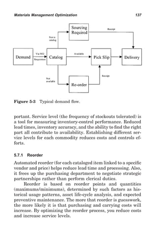
401. 380 Appendix 1
and
dF (t)
ϭ f (t)
dt
Therefore
du dR(t) dF(t)
ϭ ϭϪ ϭ Ϫf(t)
dt dt dt
Then du ϭ Ϫf (t)dt.
Substituting into ∫udv ϭ uv Ϫ ∫vdu
∞ ∞
Ύ
0
R (t)dt ϭ [tR(t)] ∞ ϩ
0 Ύ
0
tf (t)dt
∞
but limt→ ∞ tR(t) ϭ 0 when ∫0 tf(t)dt exists. Therefore the term
[tR (t)]∞ in the above equation is 0.
0
Hence
∞ ∞
Ύ
0
R (t)dt ϭ Ύ
0
tf (t)dt ϭ E(t) ϭ MTTF

402. Appendix 2: Median Ranks
When only a few failure observations are available (say, Յ12),
use is made of median rank tables (Table A.2.1).
Example: Bearing failures times (in months): 2, 3, 3.5,
4, 6. From median rank tables:
Median
rank (%)
First failure time 13.0 2 months
Second failure time 31.5 3 months
Third failure time 50.0 3.5 months
Fourth failure time 68.6 4 months
Fifth failure time 87.1 6 months
381

403. 382
Table A.2.1 Median Ranks
1 2 3 4 5 6 7 8 9 10 11 12
1 50 29.289 20.630 15.910 12.945 10.910 9.428 8.300 7.412 6.697 6.107 5.613
2 70.711 50.000 38.573 31.381 26.445 22.849 20.113 17.962 16.226 14.796 13.598
3 79.370 61.427 50.000 42.141 36.412 32.052 28.624 25.857 23.578 21.669
4 84.090 68.619 57.859 50.000 44.015 39.308 35.510 32.390 29.758
5 87.055 73.555 63.588 55.984 50.000 45.169 41.189 37.853
6 89.090 77.151 67.948 60.691 54.811 50.000 45.951
7 90.572 79.887 71.376 64.490 58.811 54.049
8 91.700 82.018 74.142 67.620 62.147
9 92.587 83.774 76.421 70.242
10 93.303 85.204 78.331
11 93.893 86.402
12 94.387
Appendix 2

404. Median Ranks 383
From a Weibull analysis:
µ ϭ 3.75 months
σ ϭ 1.5 months
Benard’s formula is a convenient and reasonable esti-
mate for the median ranks.
Cumulative probability estimator i Ϫ 0.3
ϭ
Benard’s formula N ϩ 0.4

406. Appendix 3: Censored Data
Modified Median
Hours Event Order order rank
67 F 1 1 0.13
120 S 2 — —
130 F 3 2.5 0.41
220 F 4 3.75 0.64
290 F 5 5.625 0.99
Procedure:
(n ϩ 1) ϫ Previous order number
Iϭ
1 ϩ Number of items following suspended set
385

407. 386 Appendix 3
where I ϭ increment. The first-order number remains un-
changed.
For the second, applying the equation for the increment
I, we get
(5 ϩ 1) ϫ (1)
Iϭ ϭ 1.5
1 ϩ (3)
Adding 1.5 to the previous order number 1 gives the order
number of 2.5 to the second failure:
Cumulative probability estimator i Ϫ 0.3
ϭ
Benard’s formula N ϩ 0.4
(5 ϩ 1) ϫ (2.5)
Iϭ ϭ 3.75
1 ϩ (3)
(5 ϩ 1) ϫ (3.75)
Iϭ ϭ 5.625
1 ϩ (3)
Applying Benard’s Formula to estimate median ranks for the
first failure:
1 Ϫ 0.3
Median rank ϭ ϭ .13
5 ϩ 0.4
Similarly, for the second, third, and fourth failures, re-
spectively:
2.5 Ϫ 0.3 3.75 Ϫ 0.3 5.625 Ϫ 0.3
ϭ 0.41; ϭ 0.64; ϭ 0.99.
5.4 5.4 5.4

408. Appendix 4: The Three-Parameter
Weibull Function
Failure Time of Median ranks
no. failure N ϭ 20
i ti F (t i)
1 550 3.406
2 720 8.251
3 880 13.147
4 1020 18.055
5 1180 22.967
6 1330 27.880
7 1490 32.975
8 1610 37.710
9 1750 42.626
10 1920 47.542
11 2150 52.458
12 2325 57.374
13–20 Censored data
387

409. 388 Appendix 4
The curvature suggests that the location parameter is greater
than 0.

410. Three-Parameter Weibull Function 389
Failure Time of Median ranks
no. failure N ϭ 20
i ti F (t i)
1 0 3.406
2 170 8.251
3 330 13.147
4 470 18.055
5 630 22.967
6 780 27.880
7 940 32.975
8 1060 37.710
9 1200 42.626
10 1370 47.542
11 1600 52.548
12 1775 57.374
13–20 Censored data
Now we get a line that is curved the other way, proving that
the location parameter has a value between 0 and 550. λ ϭ
375 yields a straight line, as shown in the following figure.

411. 390 Appendix 4
Failure Time of Median ranks
no. failure N ϭ 20
i ti F (t i)
1 375 3.406
2 495 8.251
3 705 13.147
4 845 18.055
5 1005 22.967
6 1155 27.880
7 1315 32.975
8 1435 37.710
9 1575 42.626
10 1745 47.542
11 1975 52.458
12 2150 57.374
13–20 Censored data
The three-parameter Weibull λ ϭ 375.

412. Appendix 5: Confidence Intervals
From the Weibull plot, we can say that at time t ϭ 7 the cumu-
lative distribution function will have a value between 30% and
73% with 90% confidence. In other words, after 7 hours in 90%
of the tests, between 30% and 73% of the batteries will have
stopped working.
If we want a confidence interval of 90% on the reliabil-
ity R(t) at the time t ϭ 7, we take the complement of the
limits on the confidence interval for F(t): (100–73, 100–30). So
the 90% confidence interval for the reliability at time t ϭ 7
hours is between 27% and 70%. Or we can say that we are
95% sure that the reliability after 7 hours will not be less than
27%.
391

413. Table A.5.1 12 Electrical Batteries
Failure Median 5% 95%
no. ranks ranks ranks ti
1 5.613 0.426 22.092 1.25
2 13.598 3.046 33.868 2.40
3 21.669 7.187 43.811 3.20
4 29.758 12.285 52.733 4.50
5 37.853 18.102 60.914 5.00
6 45.941 24.530 68.476 6.50
7 54.049 31.524 75.470 7.00
8 62.147 39.086 81.898 8.25
9–12 Still operating

414. Confidence Intervals
Table A.5.2 5% Ranks
1 2 3 4 5 6 7 8 9 10 11 12
1 5.00 2.53 1.70 1.27 1.02 0.85 0.71 0.64 0.57 0.51 0.47 0.43
2 22.36 13.054 9.76 7.64 6.28 5.34 4.62 4.10 3.68 3.33 3.05
3 36.84 24.86 18.92 15.31 12.88 11.11 9.78 8.73 7.88 7.19
4 47.24 34.26 27.13 22.53 19.29 16.88 15.00 13.51 12.29
5 54.93 41.82 34.13 28.92 25.14 22.24 19.96 18.10
6 60.70 47.91 40.03 34.49 30.35 27.12 24.53
7 65.18 52.9 45.04 39.34 34.98 31.52
8 68.77 57.09 49.31 43.56 39.09
9 71.69 60.58 52.99 47.27
10 74.11 63.56 56.19
11 76.16 66.13
12 77.91
393

415. 394
Table A.5.3 95% Ranks
1 2 3 4 5 6 7 8 9 10 11 12
1 95 77.64 63.16 52.71 45.07 39.30 34.82 31.23 28.31 25.89 23.84 22.09
2 97.47 86.46 75.14 65.74 58.18 52.07 47.07 42.91 39.42 36.44 33.87
3 98.31 90.24 81.08 72.87 65.87 59.97 54.96 50.69 47.01 43.81
4 98.73 92.36 84.68 77.47 71.08 65.51 60.66 56.44 52.73
5 98.98 93.72 87.12 80.71 74.86 69.65 65.02 60.90
6 99.15 94.66 88.89 83.13 77.76 72.88 68.48
7 99.27 95.36 90.23 85.00 80.04 75.47
8 99.36 95.90 91.27 86.49 81.90
9 99.43 96.32 92.12 87.22
10 99.49 96.67 92.81
11 99.54 96.95
12 99.57
Appendix 5

416. Appendix 6: Estimating (Fitting) the
Distribution
Maximum-likelihood estimate method:
n
Αx
΂ ΃
ˆ
β n ˆ
1/β
ln x i
Αx
i ˆ
n β
Α ln x Ϫ β ϭ 0,
1 1 i
iϭ1
n
Ϫ ˆ i ηϭ
ˆ iϭ1
n
Αx
iϭ1
ˆ
β
i
iϭ1
n
Method of least-squares estimate:
΂Α ΃
n 2
n
xi
ˆ
Αx 2
i Ϫ iϭ1
n
βϭ η ϭ eA
iϭ1 ˆ
n n
, ˆ
n Αx Αy i i
Αxy Ϫ
iϭ1
i i
iϭ1
n
iϭ1
395

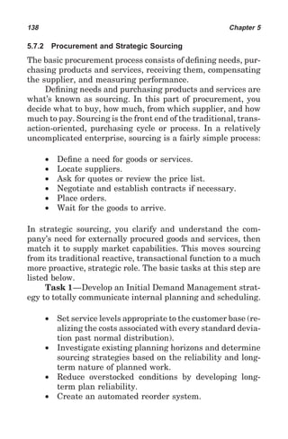
417. 396 Appendix 6
where
y i ϭ ln(t i) and x i ϭ ln[ln(1 Ϫ Median rank of y i )]
ˆ ∑y i 1 ∑x i
Aϭ Ϫ
n β n
The MLE method needs an iterative solution for the beta
estimate. Statisticians prefer maximum-likelihood estimates
to all other methods because MLE has excellent statistical
properties. They recommend MLE as the primary method.
In contrast, most engineers recommend the least-squares
method. In general, both methods should be used because each
has advantages and disadvantages in different situations.
Although MLE is more precise, for small samples it will be
more biased than rank-regression estimates (from Ref. 2 in
Chapter 9).

418. Appendix 7: Kolmogorov-Smirnov
Goodness-of-Fit Test
STEPS
1. Determine the distribution to which you want to fit
the data. Then determine the parameters of the cho-
sen distribution.
2. Determine the significance level of the test (α usually
at 1, 5 or 10%). It is the probability of rejecting the
hypothesis that the data follows the chosen distribu-
tion assuming the hypothesis is true.
3. Determine F(t i) using the parameters assumed in
step 1. F(t i ) is the value of the theoretical distribution
for failure number i.
4. ˆ
From the failure data compute F(t i ) using the median
ranks if appropriate.
397

419. 398 Appendix 7
5. Determine the maximum value of:
ˆ
|F(t i) Ϫ F(t i)|
Ά ˆ
|F(t i) Ϫ F(t iϪ1)|
ϭd ·
d Ͼ d α, we reject the hypothesis that the data can
be adjusted to the distribution chosen in step 1 (d α is
obtained for the K-S statistic table).
We have tested five items to failure. Here are the failure
times: 1, 5, 6, 8, and 10 hours. We assumed that the data fol-
lows a normal distribution and will check this assumption
with a K-S goodness-of-fit test.
SOLUTION
Estimate the parameters of the chosen distribution: Esti-
mate of
∑t i
µϭ ϭ6
n
and the estimate of
∑(t i Ϫ t)2
σ2 ϭ ϭ s2
(n Ϫ 1)
ti ˆ
F(t i) |F(t i)| ˆ
|F(t i) Ϫ F(t i)| ˆ
|F(t i) Ϫ F(t iϪ1)| d
1 0.070 0.129 0.059 0.059
5 0.390 0.314 0.076 0.261 d max 0.261
6 0.500 0.500 0.0 0.186 0.186
8 0.720 0.686 0.034 0.220 0.220
10 0.880 0.871 0.009 0.194 0.194
The values of F(t i ) are obtained from the normal distribu-
tion table. Here we are engaging in hypothesis testing. A sig-
nificance level is applied by some authority or standard gov-
erning the situation, either 0.01, 0.05, 0.10, 0.15, or 0.20.

420. K-S Goodness-of-Fit Test 399
Table A.7.1 Kolmogorov-Smirnov Critical Values
K-S level of significance (d α)
Sample
size n 0.20 0.15 0.10 0.05 0.01
1 0.900 0.925 0.950 0.975 0.995
2 0.684 0.726 0.776 0.842 0.929
3 0.565 0.597 0.642 0.708 0.828
4 0.494 0.525 0.564 0.624 0.783
5 0.446 0.474 0.510 0.565 0.669
6 0.410 0.436 0.470 0.521 0.618
7 0.381 0.405 0.438 0.486 0.577
8 0.358 0.381 0.411 0.457 0.543
9 0.339 0.360 0.388 0.432 0.514
10 0.322 0.342 0.368 0.410 0.490
11 0.307 0.326 0.352 0.391 0.468
12 0.285 0.313 0.338 0.375 0.450
13 0.284 0.302 0.325 0.361 0.433
14 0.274 0.292 0.314 0.349 0.418
15 0.266 0.283 0.304 0.338 0.404
16 0.258 0.274 0.295 0.328 0.392
17 0.250 0.266 0.286 0.318 0.381
18 0.244 0.259 0.278 0.309 0.371
19 0.237 0.252 0.272 0.301 0.363
20 0.231 0.246 0.264 0.294 0.356
25 0.21 0.22 0.24 0.27 0.32
30 0.19 0.20 0.22 0.24 0.29
35 0.18 0.19 0.21 0.023 0.27
Over 35 1.07 1.14 1.22 1.36 1.63
√n √n √n √n √n
Source: Journal of the American Statistical Association 46(53):70.
We apply our K-S statistic, 0.261, to the row for a sample
size of 5 of Table A.7.1. Assuming we wish to conform to a
significance level of 0.20, we note that 0.261 is not greater
than 0.446. That means that if we were to reject the model,
there will be a high probability (20%) that we’re wrong (in re-
jecting a good model). We therefore say that the model is not
rejected based on a 20% significance level. Frequently the less
stringent 5% significance level is applied.

422. Appendix 8: Present Value
PRESENT VALUE FORMULAE
To introduce the present-value criterion (or present dis-
counted criterion) consider the following. If a sum of money—
say, $1000—is deposited in a bank where the compound inter-
est rate on such deposits is 10% per annum, payable annually,
then after 1 year there will be $1100 in the account. If this
$1100 is left in the account for a further year, there will then
be $1210 in the account.
In symbol notation we are saying that if $L is invested
and the relevant interest rate is i% per annum, payable annu-
ally, then after n years the sum S resulting from the initial
invesment is
΂ ΃
n
i
S ϭ $L 1 ϩ (1)
100
401

423. 402 Appendix 8
Thus, if L ϭ $1000, i ϭ 10%, and n ϭ 2 years
S ϭ 1000(1 ϩ 0.1)2 ϭ $1210
The present-day value of a sum of money to be spent or
received in the future is obtained by doing the reverse calcula-
tion of that above. Namely, if $S is to be spent or received n
years in the future, and i% is the relevant interest rate, then
the present value of $S is
΂ ΃
n
1
PV ϭ $S (2)
i
1ϩ
100
where
΂ 1ϩ
1
i
100
΃ ϭ r is termed the discount factor.
Thus, the present-day value of $1210 to be received 2 years
from now is
΂ ΃
2
1
PV ϭ 1210 ϭ $1000
1 ϩ 0.1
That is, $1000 today is ‘‘equivalent’’ to $1210 2 years from now
when i ϭ 10%.
It has been assumed that the interest is paid once per
year. Interest may, in fact, be paid weekly, monthly, quarterly,
semiannually, etc., in which case the formulae (1) and (2) need
to be modified. In practice, with replacement problems it is
usual to assume that interest is payable once per year and so
Equation 2 is used in the present-value calculations.

424. Present Value 403
Figure A.8.1
It is usual to assume that the interest rate i is given as
a decimal, not in percentage terms. Equation 2 is then
written as
΂ ΃
n
1
PV ϭ $S (3)
1ϩi
An illustration of the sort of problem in which the pres-
ent-value criterion is used is the following. If a series of pay-
ments S 0, S 1, S 2 . . . S n, illustrated in Figure A.8.1, are to be
made annually over a period of n years, then the present value
of such a series is
΂ ΃ ΂ ΃ ΂ ΃
1 2 n
1 1 1
PV ϭ S 0 ϩ S 1 ϩ S2 ϩ ⋅ ⋅ ⋅ ϩ Sn (4)
1ϩi 1ϩi 1ϩi
If the payment is S j, where j ϭ 0, 1, . . . , n are equal, then
the series of payments is termed an annuity and Equation 4
becomes
΂ ΃ ΂ ΃ ΂ ΃
1 2 n
1 1 1
PV ϭ S ϩ S ϩS ϩ⋅⋅⋅ϩS (5)
1ϩi 1ϩi 1ϩi
which is a geometric progression and the sum of n ϩ 1 terms
of a geometric progression gives
΄ ΂ ΃
΅
nϩ1
1
1Ϫ
΂ ΃
1ϩi 1 Ϫ r nϩ1
PV ϭ S ϭS (6)
1Ϫr
1Ϫ
΂ ΃
1
1ϩi

425. 404 Appendix 8
If the series of payments of Equation 5 is assumed to con-
tinue over an infinite period of time, i.e., n → ∞, then from the
sum to infinity of a geometric progression we get
S
PV ϭ (7)
1Ϫr
In all the above formulae we have assumed that i remains
constant over time. If this is not a reasonable assumption,
then Equation 4 needs to be modified slightly; for example, we
may let i take the values i 1 , i 2 , . . . , in the different periods.
EXAMPLE: ONE-SHOT DECISION
To illustrate the application of the present-value criterion in
order to decide on the best of a set of alternative investment
opportunities we will consider the following problem.
A subcontractor obtains a contract to maintain special-
ized equipment for a period of 3 years, with no possibility of
an extension of this period. To cope with the work, the contrac-
tor must purchase a special-purpose machine tool. Given the
costs and salvage values shown in the table for three equally
effective machine tools, which should the contractor purchase?
We will assume that the appropriate discount factor is 0.9 and
that operating costs are paid at the end of the year in which
they are incurred.
Operating cost $
Machine Purchase Installation Salvage
tool price ($) cost ($) Year 1 Year 2 Year 3 value
A 50,000 1000 1000 1000 1000 30,000
B 30,000 1000 2000 3000 4000 15,000
C 60,000 1000 500 800 1000 35,000
For machine tool A:
Present value ϭ 50,000 ϩ 1000 ϩ 1000(0.9)
ϩ 1000(0.9)2 ϩ 1000(0.9)3 Ϫ 30,000(0.9)3
ϭ $31,570

426. Present Value 405
For machine tool B:
Present value ϭ 30,000 ϩ 1000 ϩ 2000(0.9)
ϩ 3000(0.9)2 ϩ 4000(0.9)3 Ϫ 15,000(0.9)3
ϭ $27,210
For machine tool C:
Present value ϭ 60,000 ϩ 1000 ϩ 500(0.9)
ϩ 800(0.9)2 ϩ 1000(0.9)3 Ϫ 35,000(0.9)3
ϭ $37,310
Thus equipment B should be purchased since it gives the mini-
mum present value of the costs.
FURTHER COMMENTS
In the above machine-tool-purchasing example, it will be no-
ticed that the same decision regarding the tool to purchase
would not have been reached if no account had been taken of
the time value of money. Note also that many of the figures
used in such an analysis will be estimates of future costs or
returns. When there is uncertainty about any such estimates,
or when the present-value calculation indicates several equally
acceptable alternatives (because their present values are more
or less the same), then a sensitivity analysis of some of the esti-
mates may provide information to enable an ‘‘obvious’’ decision
to be made. If this is not the case, then we may impute other
factors such as knowledge of supplier, spares availability, etc.,
to assist in reaching a decision. Of course, when estimating fu-
ture costs and returns, possible increases in materials costs,
wages, etc. (i.e., inflationary effects), should be considered.
When dealing with capital-investment decisions, a crite-
rion other than present value is sometimes used. For discus-
sion of such criteria—for example, payback period and inter-
nal rate of return—the reader is referred to the engineering
economic literature, such as Refs. 2 and 3 of the Bibliography
in Chapter 9.

428. Appendix 9: Cost of Capital
Required for Economic-Life
Calculations
Assume that the cost associated with burrowing money is an
interest charge of about 20% per annum. One of the reasons
for this high interest rate is inflation. When economic calcula-
tions are made, it is acceptable to work in terms of either
‘‘nominal’’ dollars—i.e., dollars having the value of the year
in which they are spent (or received)—or in ‘‘real’’ dollars—
i.e., dollars having present-day value. Provided that the cor-
rect cost of capital is used in the analysis, the same total dis-
counted cost is obtained whether nominal or real dollars are
used. (This does assume that inflation proceeds at a constant
annual rate.)
To illustrate the method for obtaining the cost of capital
if all calculations are done in present-day—i.e., real—dollars,
consider the following.
407

429. 408 Appendix 9
ASSUMING NO INFLATION
I put $100 in the bank today, leave it for 1 year, and the bank
will pay me 5% interest for doing so. Thus, at the end of the
year I can still buy $100 worth of goods plus an item costing
$5.00. My return for doing without my $100 for 1 year is an
item costing $5 (and I can still have goods costing $100 if I
wish).
ASSUME INFLATION AT 10% P.A.
I put $100 in the bank today. To obtain a ‘‘real’’ return of 5%
by foregoing the use of this $100 today requires that I can still
buy $100 worth of goods—which in 1 year would cost $110
since inflation occurs at 10%, plus the item originally costing
$5.00, which 1 year later would cost $5.00 ϩ 10% of $5.00,
which is $5.50. Thus, at the end of the year, I need to have
$100 ϩ $10 ϩ $5 ϩ $0.50 ϭ $115.50. The interest required on
my $100 investment, then, is
$10 ϩ $5 ϩ $0.50
ϭ θ ϩ i ϩ iθ
ϭ 10% ϩ 5% ϩ 0.5%
ϭ 15.5%
where θ ϭ inflation rate and i ϭ interest rate. Alternatively,
if the interest rate today for discounting is 15.5% and inflation
is at 10% then the ‘‘real’’ interest rate is:
iϭ
΂ ΃
1 ϩ 0.155
1 ϩ 0.10
Ϫ1
ϭ
΂ ΃ 1.155
1.10
Ϫ1
ϭ 1.05 Ϫ 1
ϭ 0.05 (or 5%)

430. Cost of Capital 409
Formally, the appropriate cost of capital when working
in present-day dollars is:
1 ϩ Cost of capital (as a decimal and with inflation)
i ϭ
1 ϩ Inflation rate (as a decimal)
AN EXAMPLE TO ILLUSTRATE THE USE OF
REAL AND NOMINAL DOLLARS
Assume we are in the year 2020:
Cost of truck in 2000 ϭ $75,000
Maintenance cost for a new truck in 2020
ϭ $5000
Maintenance cost for a 1 year old truck in 2020
ϭ $10,000
Maintenance cost for a 2 year old truck in 2020
ϭ $15,000
Assuming the real cost of capital ϭ 15%, then the total dis-
counted cost of the above series of cash flow is:
΂ ΃
1
1
$75,000 ϩ $5000 ϩ $10,000
1 ϩ .15
΂ ΃
2
1
ϩ $15,000
1 ϩ .15
ϭ $75,000 ϩ $5000 ϩ $10,000 (0.8696)
ϩ $15,000 (0.8696)2
ϭ $75,000 ϩ $5000 ϩ $8696 ϩ $11,342
ϭ $100,038
Assuming inflation now occurs at an average rate of 10% per
annum, then the cost of capital would be:
0.15 ϩ 0.10 ϩ 0.10(0.15) ϭ 0.265

431. 410 Appendix 9
The cost data would now be:
Cost of truck in 2020 ϭ $75,000
Maintenance cost of a new truck for 1 year in 2020
ϭ $5000
Maintenance cost of a 1-year-old truck for 1 year in 2021
ϭ $10,000 (1 ϩ 0.01) ϭ $11,000
Maintenance cost of a 2-year-old truck for 1 year in 2022
ϭ $15,000 (1 ϩ 0.1)2 ϭ $18,150
Using a cost of capital of 26.5%, the total discounted cost would
now be:
΂ ΃
1
1
$75,000 ϩ $5000 ϩ $11,000
1 ϩ 0.265
΂ ΃
2
1
ϩ $18,150
1 ϩ 0.265
ϭ $75,000 ϩ $5000 ϩ $11,000 (0.7905)
ϩ $18,150 (0.6249)
ϭ $75,000 ϩ $5000 ϩ $8696 ϩ $11,343
ϭ $100,038
(which is identical to the result obtained when present-day
dollars were used along with an ‘‘uninflationary’’ cost of cap-
ital.
EQUIVALENT ANNUAL COST
The economic-life model gives a dollar cost that is a conse-
quence of an infinite chain of replacements, or by modification
(see following) for the first N cycles. To ease interpretation
of this total discounted cost, it is useful to convert the total
discounted costs associated with the economic life to an Equiv-
alent Annual Cost (EAC).

432. Cost of Capital 411
In the calculations performed above, the total discounted
cost over the 3 years was $100,038 when the cost of capital
was 15%. Using a quantity called the “capital recovery factor”
(CRF) it is possible to convert the $100,038 to an equivalent
annual cost. The formula for calculating the CRF is:
i(1 ϩ i)n
CRF ϭ
(1 ϩ i)n Ϫ 1
Rather than use the above formula, most books dealing with
financial analysis include tables of CRFs for a variety of inter-
est rates. In such tables one would find for i ϭ 15% and n ϭ 3
years the CRF ϭ 0.4380 and the EAC is $100,038 (0.4380) ϭ
$43,816.644 p.a. This means that a constant payment of
$43,816.644 p.a. would result in a total discounted cost (TDC)
of $100,038 if the cost of capital is taken at 15%.
Check:
΂ ΃
1
1
TDC ϭ $43,816.644
1 ϩ 0.15
΂ ΃
2
1
ϩ $43,816.644
1 ϩ 0.15
΂ ΃
3
1
ϩ $43,816.644
1 ϩ 0.15
ϭ $38,101.43 ϩ $33,131.678 ϩ $28,810.152
ϭ $100,043
(given rounding errors, this is equal to $100,038).

434. Appendix 10: Optimal Number
of Workshop Machines to Meet
a Fluctuating Workload
STATEMENT OF PROBLEM
From time to time, jobs requiring the use of workshop ma-
chines (say, lathes) are sent from various production facilities
within an organization to the maintenance workshop. De-
pending on the workload of the workshop, these jobs will be
returned to production after some time has elapsed. The prob-
lem is to determine the optimal number of machines that min-
imizes the total cost of the system. This cost has two compo-
nents: the cost of the workshop facilities and the cost of
downtime incurred by jobs waiting in the workshop queue and
then being repaired.
413

435. 414 Appendix 10
CONSTRUCTION OF MODEL
1. The arrival rate of jobs to the workshop requiring
work on a lathe is Poisson-distributed with arrival
rate λ.
2. The service time a job requires on a lathe is negative-
exponentially distributed with mean 1/µ.
3. The downtime cost per unit time for a job waiting in
the system (i.e., being served or in the queue) is C d.
4. The cost of operation per unit time for one lathe (ei-
ther operating or idle) is C l.
5. The objective is to determine the optimal number of
lathes n to minimize the total cost per unit time C(n)
of the system.
C(n) ϭ Cost per unit time of the lathes
ϩ Downtime cost per unit time due to
jobs being in the system
Cost per unit time of the lathes
ϭ Number of lathes
ϫ Cost per unit time per lathe
ϭ nC 1
Downtime cost per unit time of jobs
being in the system
ϭ Average wait in the system per job
ϫ Arrival rate of jobs in the system per unit time
ϫ Downtime cost per unit time per job
ϭ W s λC d
where W s ϭ mean wait of a job in the system. Hence
C(n) ϭ nC l ϩ W s λC d
This is a model of the problem relating number of machines
n to total cost C(n).

436. Appendix 11: Optimal Size of a
Maintenance Workforce to Meet a
Fluctuating Workload, Taking into
Account Subcontracting
Opportunities
STATEMENT OF PROBLEM
The workload for the maintenance crew is specified at the be-
ginning of a period—say, a week. By the end of the week the
entire workload must be completed. The size of the workforce
is fixed—there is a fixed number of manhours available per
week. If demand at the beginning of the week requires fewer
manhours than the fixed capacity, no subcontracting takes
place. If, however, the demand is greater than the capacity,
then the excess workload is subcontracted and returned from
the subcontractor by the end of the week. Two sorts of costs
are incurred:
415

437. 416 Appendix 11
1. Fixed cost depending on the size of the workforce.
2. Variable cost depending on the mix of internal/exter-
nal workload
As the fixed cost is increased through increasing the size of
the workforce, there is less chance of subcontracting being nec-
essary. However, there may often be occasions when fixed
costs will be incurred yet demand low, i.e., considerable under-
utilization of workforce. The problem is to determine the opti-
mal size of the workforce to meet a fluctuating demand in or-
der to minimize expected total cost per unit time.
CONSTRUCTION OF MODEL
1. The demand per unit time is distributed according to
a probability density function f (r ), where r is the
number of jobs.
2. The average number of jobs processed per worker per
unit time is m.
3. The total capacity of the workforce per unit time is
nm, where n is the number of staff in the workforce.
4. The average cost of processing one job by the work-
force is C 1.
5. The average cost of processing one job by the subcon-
tractor is C s .
6. The fixed cost per man per unit time is C f .
The basic conflicts of this problem are illustrated in Fig-
ure A.11.1, in which it is seen that the expected total cost per
unit time C(n) is
C(n) ϭ Fixed cost per unit time
ϩ Variable internal processing per unit time
ϩ Variable subcontracting processing
cost per unit time

438. Optimal Size of Workforce 417
Figure A.11.1
Fixed cost per unit time ϭ Size of workforce
ϫ Fixed cost per person
ϭ nC f
Variable internal processing cost per unit time ϭ
Average number of jobs processed
internally per unit time
ϫ Cost per job
Now, number of jobs processed internally per unit time will be
1. Equal to the capacity when demand is greater than
capacity
2. Equal to demand when demand is less than, or equal
to, capacity
∞
Probability of no. 1 ϭ Ύ nm
f (r )dr
∞
Probability of no. 2 ϭ Ύ Ύ
nm
f (r )dr ϭ 1 Ϫ f (r )dr
Ϫ∞ nm

439. 418 Appendix 11
When no. 2 occurs, the average demand will be
ΗΎ
∞
Ύ
nm
f (r )dr f (r )dr
0 0
Therefore, variable internal processing cost per unit time is
΂ Ύ
΃
nm
∞ rf (r)dr
nmΎ f (r )dr ϩ Ύ
nm
0
rf (r)dr C w
Ύ
nm
nm 0
rf (r)dr
0
Variable subcontracting processing cost per unit time ϭ
Average number of jobs processed
externally per unit time
ϫ Cost per job
Now, the number of jobs processed externally will be
1. Zero when the demand is less than the workforce ca-
pacity
2. Equal to the difference between demand and capacity
when demand is greater than capacity.
Ύ
nm
Probability of no. 1 ϭ f (r )dr
0
∞
Probability of no. 2 ϭ Ύ Ύ
nm
f(r )dr ϭ 1 Ϫ f (r )dr
nm 0
When no. 2 occurs, the average number of jobs subcontracted
is:
ΗΎ
∞ ∞
Ύ
nm
(r Ϫ nm)f (r )dr
nm
f (r )dr
Therefore, variable subcontracting processing cost per unit
time is

440. Optimal Size of Workforce 419
΂ ΃
∞
Ύ (r Ϫ nm)f(r)dr ∞
Ύ Ύ
nm
0ϫ f (r )dr ϩ nm
∞
f (r)dr C s
Ύ
0 nm
f (r)dr
nm
Therefore
΂ ΃
∞
Ύ Ύ
nm
c(n) ϭ nC f ϩ nm f (r)dr ϩ f (r )dr C w
rm 0
∞
ϩ Ύ nm
(r Ϫ nm)f (r)dr
This is a model of the problem relating workforce size n to
total cost per unit time C(n).

442. Appendix 12: Fuzzy Logic
Fuzzy logic terminology: degree of membership, universe of
discourse, membership function/fuzzy subset. In Figure A.12.1,
as an example, the universe of discourse is the set of people.
To each person in the universe of discourse, we assign a degree
Figure A.12.1
421

443. 422 Appendix 12
of membership in the fuzzy subset TALL. George, who is 4′ 8″
(by substitution in the membership function above), has de-
gree of membership in TALL of 0. Sam, 5′ 9″, has a degree of
tallness of 0.38. Kareem, at 7′ 2″, is tall: dom. 1.0.

444. Appendix 13: Neural Nets
Here is the neural net example from Chapter 10 (which illus-
trates many of the concepts) taken from Donald R. Tveter’s
manual to the professional version of his Backprop Algorithm
software package (Ref. 4 in Chapter 10). A three-layer network
to provide XOR functionality after suitable ‘‘training’’ is de-
scribed below (how it gets trained is explained later).
A THREE-LAYER MULTILAYER
PERCEPTRON
Figure A.13.1 is a 2-1-1 network (multilayer perceptron, or
MLP) with extra input-output connections (better for some
problems like XOR). To get an answer for the case x ϭ 1 and
423

445. 424 Appendix 13
Figure A.13.1
y ϭ 0, first compute the sum of inputs to the hidden layer neu-
ron h: s ϭ (1 ϫ 7.1) ϩ (1 ϫ Ϫ2.76) ϩ (0 ϫ 7.1) ϭ 4.34. Then
apply the activation function v ϭ 1/(1 ϩ eϪS ) to compute the
activation value, v ϭ 1/(1 ϩ eϪ4.34) ϭ 0.98%. The output neuron
is computed similarly: s ϭ (1 ϫ Ϫ4.95) ϩ (0 ϫ Ϫ4.95) ϩ (0.98%
ϫ 10.9) ϩ (1 ϫ Ϫ3.29) ϭ 2.52 and v ϭ 0.926. Of course, 0.926
is not quite 1, but for this example it’s close enough. There are
other activation functions you can use that make it easier to
get closer to the targets. Here is the
net j ϭ Αw o
iϭ1,n
ij i o j ϭ f (net j)
where net j ϭ net input to neuron j ; f ϭ the activation function;
w ij ϭ the weight between neurons j and i. Now let’s see how
the network gets trained. The method is back-propagation.
These are the steps:
1. Start with arbitrary values for w ij . In this case the
network weights all start out at 0 (a bad idea in gen-
eral, but it works here). The activation values for the

446. Neural Nets 425
hidden and output neurons are both 0.5 as calculated
by the above two formulas.
2. Put one of the patterns to be learned on the input
units.
3. Find the values of the hidden and output units.
4. Find out how large the error is on the output unit.
5. Use one of the back-propagation formulas to adjust
the weights leading into the output unit.
6. Use another formula to find the errors for the hidden
layer unit.
7. Adjust the weights leading into the hidden layer unit
via another formula.
8. Repeat steps 2 to 7 for the second, third, and fourth
XOR patterns.
Even after all these changes, the answers will be only a little
closer to the right answers, and the whole process must be
repeated many times. Each time all the patterns in the prob-
lem are used is an epoch. Here are the formulas:
δ k ϭ (t k Ϫ o k)f ′(net k)
1
fϭ
1 ϩ eϪnetk
f ′ ϭ o k(1 Ϫ o k )
w jk ← w jk ϩ ηδ k o j
where: δ k ϭ error signal; t k ϭ target for unit k; f ′ ϭ derivative
of activation function f, η ϭ learning rate ϭ 0.1. Here is the
first set of calculations:
δz ϭ (1 Ϫ 0.5) ∗ 0.5 ∗ (1 Ϫ 0.5) ϭ 0.125
w xz ← 0 ϩ 0.1 ∗ 0.125 ∗ 1 ϭ 0.0125
w yz ← 0 ϩ 0.1 ∗ 0.125 ∗ 0 ϭ 0
w hz ← 0 ϩ 0.1 ∗ 0.125 ∗ 0.5 ϭ 0.00625
wbz ← 0 ϩ 0.1 ∗ 0.125 ∗ 1 ϭ 0.0125

447. 426 Appendix 13
δ j ϭ f ′(net j) Αδ w
k
k kj
where δ j ϭ error for a hidden unit j. Therefore, δ h ϭ o h(1 Ϫ
o h)δ zh ϭ 0.5 ∗ (1 Ϫ 0.5) ∗ 0.125 ∗ 0.00625 ϭ 0.000195313.
w ij ← w ij ϩ ηδ j o i is weight-change formula between
hidden unit j and input unit i. Therefore, w hx ϭ 0 ϩ
0.1 ∗ 0.000195313 ∗ 1 ϭ 0.0000195313; w hbh ϭ 0 ϩ 0.1 ∗
0.000195313 ∗ 1 ϭ 0.0000195313. The activation value for the
output layer will now calculate to 0.507031, a long way from
our target. If we do the same for the other three patterns we
get:
x y z desired z actual
1 0 1 0.499830
0 0 0 0.499893
0 1 1 0.499830
1 1 0 0.499768
The eight-step backprop training algorithm as given
above, although it works, is, strictly speaking, considered
wrong by mathematicians. Rather than changing the weights
leading into the output layer before propagating the error
back, it is mathematically more rigorous to compute the
weight changes for the upper layer of weights and then, with-
out changing them, compute weight changes for the lower
layer of weights. Then, with all the changes in hand, make
the changes to both sets.
Sadly, to get the outputs to within 0.1 requires 20,862
iterations (epochs)—a very long time, especially for such a
short problem. Fortunately, a lot of things can be done to speed
up the training so that the number of epochs can be reduced
to around 12–20. The simplest would be to increase the learn-
ing rate η (Figure A.13.2).

448. Neural Nets 427
Figure A.13.2
FAILURE OF A NEURAL NET TO TRAIN
An unfortunate problem with back-propagation is that, when
the learning rate is too large, the training can fail the figure
above. In this case, with η ϭ 3 after 10,000 epochs (iterations),
x ϭ 1, y ϭ 1 resulted in z ϭ 1, which is not an exclusive or.
The geometric interpretation (see Figure A.13.2) is that when
the network tries to make the error go down, it may get stuck
in a valley that is not the lowest possible valley. That is a local
minimum, which is not the global minimum that would give
perfect results. Once you go down into a shallow valley, if there
is no path downhill that will get you to the deeper valley you
are permanently stuck with a bad answer. There are ways to
break out of a local minimum, but in real-world problems you
never know when you’ve found the best (global) minimum. You
only hope to get a very deep minimum.

450. Appendix 14: Optimal Interval
Between Preventive Replacements
of Equipment Subject to
Breakdown
STATEMENT OF PROBLEM
Equipment is subject to sudden failure, and when failure oc-
curs the equipment must be replaced. Since failure is unex-
pected, it is not unreasonable to assume that a failure replace-
ment is more costly than a preventive replacement. For
example, when a preventive replacement is planned, arrange-
ments are made to perform it without unnecessary delays; a
failure may cause damage to other equipment. To reduce the
number of failures, preventive replacements can be scheduled
to occur at specified intervals. However, a balance is required
between the amount spent on the preventive replacements
and their resulting benefits, i.e., reduced failure replacements.
429

451. 430 Appendix 14
In this appendix it will be assumed, not unreasonably,
that we are dealing with a long period of time over which the
equipment is to be operated and relatively short intervals be-
tween the preventive replacements. When this is the case, we
need consider only one cycle of operations and develop a model
for the cycle. If the interval between the preventive replace-
ments is long, it is necessary to use the discounting approach
and the series of cycles must be included in the model.
The replacement policy calls for preventive replacements
to occur at fixed intervals of time and failure replacements to
occur when necessary, and we want to determine the optimal
interval between the preventive replacements to minimize
the total expected cost of replacing the equipment per unit
time.
CONSTRUCTION MODEL
1. C p is the cost of a preventive replacement.
2. C j is the cost of a failure replacement.
3. f(t) is the probability density function of the equip-
ment’s failure times.
4. The replacement policy is to perform preventive re-
placements at constant intervals of length t p, irre-
spective of the age of the equipment, and failure re-
placements occur as many times as required in
interval (0, t p). The policy is illustrated in Figure
A.14.1.
Figure A.14.1

452. Intervals Between Equipment Replacements 431
5. The objective is to determine the optimal interval be-
tween preventive replacements to minimize the total
expected replacement cost per unit time.
The total expected cost per unit time for preventive re-
placement at time t p, denoted C(t p), is
Total expected cost in interval (0, t p)
C(t p) ϭ
Length of interval
Total expected cost in interval (0, t p) ϭ Cost of a preventive
replacement ϩ Expected cost of failure replacements ϭ C p ϩ
C f H(t p) where H(t p) is the expected number of failures in inter-
val (0, t p).
Length of interval ϭ t p
Therefore
C p ϩ C f H(t p)
C(t p) ϭ
tp
This is a model of the problem relating replacement interval
t p to total cost C(t p).

454. Appendix 15: Optimal Preventive
Replacement Age of Equipment
Subject to Breakdown
STATEMENT OF PROBLEM
This problem is similar to that of Appendix 14 except that in-
stead of making preventive replacements at fixed intervals,
thus incurring the possibility of performing a preventive re-
placement shortly after a failure replacement, the time at
which the preventive replacement occurs depends on the age
of the equipment. When failure occurs, failure replacements
are made.
Again, the problem is to balance the cost of the preventive
replacements against their benefits. We do this by determin-
ing the optimal preventive replacement age for the equipment
to minimize the total expected cost of replacements per unit
time.
433

455. 434 Appendix 15
Figure A.15.1
CONSTRUCTION OF MODEL
1. C p is the cost of a preventive replacement.
2. C f is the cost of a failure replacement.
3. f(t) is the probability density function of the failure
times of the equipment.
4. The replacement policy is to perform preventive re-
placements once the equipment has reached a speci-
fied age at t p, plus failure replacements when neces-
sary. The policy is illustrated in Figure A.15.1.
5. The objective is to determine the optimal replace-
ment age of the equipment to minimize the total ex-
pected replacement cost per unit time.
In this problem, there are two possible cycles of operation:
one cycle is determined by the equipment’s reaching its
planned replacement age t p, the other by the equipment’s ceas-
ing to operate due to a failure occurring before the planned
replacement time. These two possible cycles are illustrated in
Figure A.15.2.
Figure A.15.2

456. Optimal Preventive Replacement Age 435
The total expected replacement cost per unit time C(t p) is
Total expected replacement cost per cycle
C(t p) ϭ
Expected cycle length
Total expected replacement cost per cycle
ϭ Cost of a preventive cycle
ϫ Probability of a preventive cycle
ϩ Cost of failure cycle
ϫ Probability of a failure cycle
ϭ C pR(t p) ϩ C f [1 Ϫ R(t p)]
Remember: if f (t) is as illustrated in Figure A.15.3, then the
probability of a preventive cycle equals the probability of fail-
ure occurring after time t p ; that is, it is equivalent to the
shaded area, which is denoted R(t p).
The probability of a failure cycle is the probability of a
failure occurring before time t p, which is the unshaded area
area of Figure A.15.3. Since the area under the curve equals
unity, then the unshaded area is [1 Ϫ R(t p)].
Expected cycle length ϭ Length of a preventive cycle
ϫ Probability of a preventive cycle
ϩ Expected length of a failure cycle
Figure A.15.3

457. 436 Appendix 15
Figure A.15.4
ϫ Probability of a failure cycle
ϭ t p ϫ R(t p)
ϩ (Expected length of a failure cycle) ϫ [1 Ϫ R(t p)]
To determine the expected length of a failure cycle, con-
sider Figure A.15.4. The mean time to failure of the complete
distribution is
∞
Ύ
Ϫ∞
tf(t)dt
which for the normal distribution equals the mode (peak) of
the distribution. If a preventive replacement occurs at time t p,
then the mean time to failure is the mean of the shaded por-
tion of Figure A.15.4 since the unshaded area is an impossible
region for failures. The mean of the shaded area is
Ύ
tp
tf(t)dt
Ϫ∞ 1 Ϫ R(t p)
denoted M(t p). Therefore, the expected cycle length ϭ t p ϫ
R(t p) ϩ M(t p) ϫ [1 Ϫ R(t p)]
C p ϫ R(t p) ϩ C f ϫ [1 Ϫ R(t p)]
C(t p) ϭ
t p ϫ R(t p) ϩ M(t p) ϫ [1 Ϫ R(t p)]
This is now a model of the problem relating replacement age
t p to total expected replacement cost per unit time.

458. Appendix 16: Optimal Preventive
Replacement Age of Equipment
Subject to Breakdown, Taking into
Account Time Required to Effect
Failure and Preventive
Replacements
STATEMENT OF PROBLEM
The problem definition is identical to that of Appendix 15 ex-
cept that, instead of assuming that the failure and preventive
replacements are made instantaneously, the time required to
make these replacements is taken into account.
The optimal preventive replacement age of the equip-
ment is again taken as the age that minimizes the total ex-
pected cost of replacements per unit time.
437

459. 438 Appendix 16
Figure A.16.1
CONSTRUCTION OF MODEL
1. C p is the cost of a preventive replacement.
2. C f is the cost of a failure replacement.
3. Tp is the time required to make a preventive replace-
ment.
4. Tf is the time required to make a failure replacement.
5. f(t) is the probability density function of the failure
times of the equipment.
6. M(t p) is the mean time to failure when preventive re-
placement occurs at time t p.
7. The replacement policy is to perform a preventive re-
placement once the equipment has reached a speci-
fied age at t p, plus failure replacements when neces-
sary. The policy is illustrated in Figure A.16.1.
8. The objective is to determine the optimal preventive
replacement age of the equipment to minimize the to-
tal expected replacement cost per unit time.
As was the case for the problem in Appendix 15, there
are two possible cycles of operation, which are illustrated in
Figure A.16.2.
The total expected replacement cost per unit time, de-
noted C(t p), is:
Total expected replacement cost per cycle
C(t p) ϭ
Expected cycle length

460. Equipment Age and Replacement Time 439
Figure A.16.2
Total expected replacement cost per cycle:
ϭ C p ϫ R(t p) ϩ C f [1 Ϫ R(t p)]
Expected cycle length:
ϭ Length of a preventive cycle
ϫ Probability of a preventive cycle
ϩ Expected length of a failure cycle
ϫ Probability of a failure cycle
ϭ (t p ϩ T p)R(t p) ϩ [M(t p) ϩ T f ] [1 Ϫ R(t p)]
C pR(t p) ϩ C f [1 Ϫ R(t p)]
C(t p) ϭ
(t p ϩ T p)R(t p) ϩ [M(t p) ϩ T f ] [1 Ϫ R(t p)]
This is a model of the problem relating preventive replace-
ment age t p to the total expected replacement cost per unit
time.

462. Appendix 17: Optimal Replacement
Interval for Capital Equipment:
Minimization of Total Cost
STATEMENT OF PROBLEM
This problem is introduced in Section 11.3. The objective is
to determine the replacement interval that minimizes the to-
tal cost of maintenance and replacement over a long period
where the trend in costs is taken to be discrete, rather than
continuous.
CONSTRUCTION OF MODEL
1. A is the acquisition cost of the capital equipment.
2. C i is the cost of maintenance in the ith period from
441

463. 442 Appendix 17
new, assumed to be paid at the end of the period i ϭ
1, 2, . . . , n.
3. S i is the resale value of the equipment at the end of
the ith period of operation i ϭ 1, 2, . . . , n.
4. r is the discount rate.
5. n is the age in periods of the equipment when replaced.
6. C(n) is the total discounted cost of maintaining and
replacing the equipment (with identical equipment)
over a long period of time with replacements oc-
curring at intervals of n periods.
7. The objective is to determine the optimal interval be-
tween replacements to minimize total discounted
costs C(n).
The replacement policy is illustrated in Figure A.17.1.
Consider first the cycle of operation. The total discounted
cost over the first cycle of operation, with equipment already
installed, is
C 1(n) ϭ C 1 r ϩ C 2 r 2 ϩ C 3 r 3 ϩ ⋅ ⋅ ⋅ ϩ C n r n ϩ Ar n Ϫ S nr n
n
ϭ ΑCr
iϭ1
i
i
ϩ r n (A Ϫ S n)
For the second cycle, the total cost discounted to the start of
the second cycle is
Figure A.17.1

464. Optimal Replacement Interval 443
n
C 2(n) ϭ ΑCr
iϭ1
i
i
ϩ r n (A Ϫ S n)
Similarly, the total costs of the third and fourth cycle, and
so on, discounted back to the start of their cycle, can be ob-
tained.
The total discounted costs, when discounting is taken to
the start of the operation, i.e., at time 0, is
C(n) ϭ C 1 (n) ϩ C 2 (n)r n ϩ C 3 (n)r 2n ϩ ⋅ ⋅ ⋅ ϩ C n (n)r (nϪ1)n ϩ ⋅ ⋅ ⋅
Since C 1 (n) ϭ C 2 (n) ϭ C 3 (n) ϭ ⋅ ⋅ ⋅ ϭ C n (n) ϭ . . . , we have a
geometric progression that gives, over an infinite period:
n
C 1(n)
ΑCr i
i
ϩ r n (A Ϫ S n)
C(n) ϭ ϭ iϭ1
1 Ϫ rn 1 Ϫ rn
This is a model of the problem relating replacement interval
n to total costs.

466. Appendix 18: The Economic-Life
Model Used in PERDEC
The economic life model used in PERDEC is:
n
ΑCr
΄ ΅
Aϩ i
i
Ϫ S nr n
EAC(n) ϭ iϭ0
∗i
1 Ϫ rn
where
A ϭ acquisition cost
C i ϭ O&M costs of equipment in its ith year of life, as-
suming payable at the start of year, i ϭ 1, 2, . . . , n
r ϭ Discount factor
S n ϭ Resale value of equipment of age n years
n ϭ Replacement age
C(n) ϭ Total discounted cost for a chain of replacements
every n years
445

468. Appendix 19: Economic Life of
Passenger Buses
The purpose of this appendix is to demonstrate how the stan-
dard economic life model for equipment replacement can be
modified slightly to enable the economic life of buses to be de-
termined, taking into account declining utilization of a bus
over its life. Specifically, new buses are highly utilized to meet
base load demand while older buses are used to meet peak
demands, such as during rush hour.
The case study describes a fleet of 2000 buses whose an-
nual fleet demand is 80 million kilometers. The recommenda-
tions resulting from the study were implemented and substan-
tial savings were reported.
447

469. 448 Appendix 19
INTRODUCTION
The study took place in Montreal, Canada, where Montreal’s
Transit Commission is responsible for providing bus services
to approximately 2 million people. To meet the bus schedules
requires a fleet of 2000 buses undertaking approximately
80,000,000 kilometers/year. Montreal has the third largest
fleet of North American bus operators, behind New York City
and Chicago. The bulk of the buses used in Montreal were
standard 42-seat GMC buses.
The objective of the study was to analyze bus operations
and maintenance costs to determine the economic life of a bus
and to identify a steady-state replacement policy, i.e., one in
which a fixed proportion of the fleet would be replaced on an
annual basis.
THE ECONOMIC-LIFE MODEL
Figure A.19.1 illustrates the standard conflicts associated
with capital-equipment replacement problems.
The standard economic life model is
Figure A.19.1

470. Economic Life of Buses 449
n
A ϩ C1 ϩ ΑCr i
iϪ1
Ϫ Snr n
C(n) ϭ iϭ2
1 Ϫ rn
where
A ϭ Acquisition cost
C 1 ϭ Operations and maintenance (O&M) cost of a bus
in its first year of life
C i ϭ O&M cost of a bus in its ith year of life, assuming
payable at the start of the year, i ϭ 2, 3, . . . , n
r ϭ Discount factor
S n ϭ Resale value of a bus of age n years
n ϭ Replacement age
C(n) ϭ Total discounted cost for a chain of replacements
every n years
The total discounted cost can be converted to an Equivalent
Annual Cost (EAC) by the Capital Recovery Factor, which in
this case is i, the interest rate appropriate for discounting.
Note:
1
rϭ
1ϩi
DATA ACQUISITION
Acquisition cost: In terms of 1980 dollars, the acquisition cost
of a bus was $96,330.
Resale value: The policy being implemented by Montreal
Transit was replacement of a bus on a 20-year-old cycle, at
which age the value of the bus was $1000. Because there was
considerable uncertainty in the resale value of a bus, for pur-
poses of the study two extremes were evaluated: a high and
low trend in resale value (Tables A.19.1 and A.19.2).

471. 450 Appendix 19
Table A.19.1 High
Trend in Resale Value
Resale
Replacement value
age (years) ($)
1 77,000
2 65,000
3 59,000
4 54,000
5 50,000
6 46,000
7 42,000
8 38,000
9 34,000
10 31,000
11 28,000
12 25,000
13 22,000
14 19,000
15 16,000
16 13,000
17 10,000
18 7,000
19 4,000
20 1,000
INTEREST RATE
The interest rate appropriate for discount was uncertain. In
the study a range (0% to 20%) was used to check the sensitivity
of the economic life to variations in interest rate. The major
conclusions of the study were based on an ‘‘inflation fee’’ inter-
est rate of 6%.
OPERATIONS AND MAINTENANCE COST
O&M costs are influenced by both age of a bus and its cumula-
tive utilization. O&M data were obtained for six cost catego-

472. Economic Life of Buses 451
Table A.19.2 High
Trend in Resale Value
Replacement Resale
age (years) value ($)
1 2000
2 2000
3 2000
4 2000
5 2000
6 2000
7 2000
8 2000
9 2000
10 2000
11 2000
12 2000
13 2000
14 2000
15 2000
16 2000
17 2000
18 2000
19 2000
20 1000
ries: fuel, lubrication, tires, oil, parts, and labor. Analysis of
the costs identified the following trend:
΂ ΃
2
k
c(k) ϭ 0.302 ϩ 0.723
106
where
k ϭ Cumulative kilometers traveled by the bus since
new
c(k) ϭ Trend in O&M cost in $/kilometer for a bus of age
k kilometers

473. 452 Appendix 19
Figure A.19.2
BUS UTILIZATION
Figure A.19.2 shows the trend line that was fitted to the rela-
tionship between bus utilization (km/yr) and bus age (newest
to oldest). The reason for this relationship is that new buses
are highly utilized to meet base load requirements, with the
older buses being used to meet peak demands.
In the analysis that was undertaken, it was assumed that
the relationship identified in Figure A.19.2 would be indepen-
dent of the replacment age of the bus. For example, using the
present policy of replacing buses on a 20-year cycle, in a steady
state, 2000/20 ϭ 100 buses would be replaced annually. The
total work done by the newest 100 buses in their first year of
life would then be:
100
∫ Y dk ϭ 8,636,059 kilometers
0
ϭ 86,361 km/bus
SOLVING THE MODEL
If the economic replacement age of a bus is set at 20 years,
then C(20) can be evaluated using the previously cited data

474. Economic Life of Buses 453
Figure A.19.3
and converting the annual utilization to annual cost by inte-
grating the cost trend c(k) over the appropriate utilization
range. Thus for a bus in its first year of life the O&M cost
would be:
΂ ΃
2
Ύ
86361
k
0.302 ϩ 0.723 dk
0 106
Similarly, the O&M costs for the remaining 19 years can be
calculated and inserted into the economic-life model C(n) to
enable C(20) to be calculated. The whole process is then re-
peated for other possible replacement ages to identify the opti-
mal n. Figure A.19.3 shows the results when i ranges from 0%
to 20% and the low trend in resale value is used.

475. 454 Appendix 19
CONCLUSIONS
Montreal Transit decided to implement a 3-year bus purchase
policy on the basis of a 16-year replacement age. The resultant
savings approximated $4 million/year. The class of problem
discussed here is typical of those found in many transport op-
erations, for example:
• Haulage fleets undertaking both long-distance and lo-
cal deliveries—new vehicles are used on long-haul
routes; as they age, they are relegated to local delivery
work.
• Stores with their own fleets of delivery vehicles, with
peak demands around Christmas. The older vehicles
in the fleet are retained to meet these predictable de-
mands. Because of this unequal utilization, it is neces-
sary to evaluate the economic life of the vehicle by
viewing the fleet as a whole rather than focus on indi-
vidual vehicles.
REFERENCES
1. B. W. Simms, B. G. Lamarre, A. K. S. Jardine, A. Boudreau.
Optimal Buy, Operate and Sell Policies for Fleets of Vehicles.
European Journal of Operational Research 1984; 15(2):183–
195. (This paper discusses a dynamic programming/linear pro-
gramming approach to the problem that enabled alternative uti-
lization policies to be incorporated into the model.)
2. AGE/CON User’s Manual. www.oliver-group.com (AGE/CON is
a software package used for vehicle fleet replacement decisions.
It includes the routines for handling problems of the class de-
scribed in this appendix).

476. Appendix 20: Optimal Replacement
Age of an Asset, Taking into
Account Tax Considerations
The formula is
΂ ΃΅
i
΄
1ϩ
td 2
NPV(k) ϭ A 1 Ϫ
iϩd 1ϩi
Ϫ
΂
itA 1 Ϫ
d
2΃(1 Ϫ d)kϪ1
(i ϩ d)(1 ϩ i)k
S (1 Ϫ t)
Ϫ k
(1 ϩ i)k
k
(1 Ϫ t)
ϩ Α C (1 ϩ i)
jϭ1
j jϪ1
455

477. 456 Appendix 20
where
i ϭ Interest rate
d ϭ Capital Cost Allowance rate
t ϭ Corporation tax rate
A ϭ Acquisition cost
Sk ϭ Resale price
Cj ϭ O&M cost in the jth year
NPV(k) ϭ Net Present Value in the kth year
A(1 Ϫ d/2)(1 Ϫ d)kϪ1 is the nondepreciated capital cost.
The equivalent annual cost (EAC) is then obtained by
multiplying the NPV(k) by the Capital Recovery Factor
i(1 ϩ i)k
(1 ϩ i)k Ϫ 1

478. Appendix 21: Optimal Replacement
Policy for Capital Equipment,
Taking into Account Technological
Improvement—Infinite
Planning Horizon
STATEMENT OF PROBLEM
For this replacement problem, it is assumed that, once the
decision has been made to replace the current asset with
the technologically improved equipment, this equipment will
continue to be used and a replacement policy (periodic) will
be required for it. It will also be assumed that replacement
will continue to be made with the technologically improved
equipment. Again we wish to determine the policy that mini-
mizes total discounted costs of maintenance and replace-
ment.
457

479. 458 Appendix 21
CONSTRUCTION OF MODEL
1. n is the economic life of the technologically improved
equipment.
2. C p,t is the maintenance cost of the present equipment
in the ith period from now, payable at time i: i ϭ 1,
2, . . . , n.
3. S p,t is the resale value of the present equipment at
the end of the ith period from now; i ϭ 1, 2, . . . , n.
4. A is the acquisition cost of the technologically im-
proved equipment.
5. C t,j is the maintenance cost of the technologically im-
proved equipment in the jth period after its installa-
tion and payable at time j; j ϭ 1, 2, . . . , n.
6. S t,j is the resale value of the technologically improved
equipment at the end of its jth period of operation;
j ϭ 0, 1, 2, . . . , n. ( j ϭ 0 is included so that we can
then define S t,o ϭ A. This then enables Ar n in the
model to be canceled if no change is made). Note that
it is assumed that, if a replacement is to be made at
all, it is with the technologically improved equip-
ment. This is not unreasonable since it may be that
the equipment currently in use is no longer on the
market.
7. r is the discount factor.
8. The replacement policy is illustrated in Figure A.21.1.
The total discounted cost over a long period of time with
replacement of the present equipment at the end of T period
of operation, followed by replacements of the technologically
improved equipment at intervals of n, is
C(T, n) ϭ Costs over interval (0, T ) ϩ Future costs
n
Costs over interval (0, T) ϭ ΑC
iϭ1
p,t r i Ϫ S p,T r T ϩ Ar T

480. Replacement and Technological Improvement 459
Figure A.21.1
Future costs, discounted to time T, can be obtained by the
method described in Appendix 17, where the economic life of
equipment is calculated. We replace C i with C t,j to obtain
n
ΑC t,j r i ϩ r n(A Ϫ S n)
C(n) ϭ iϭ1
1 Ϫ rn
Therefore, C(n) discounted to time zero is C(n)r T and
n
ΑC
΂ ΃
T t,j r i ϩ rn(A Ϫ S n)
C(T, n) ϭ ΑC
iϭ1
p,t r i Ϫ S p,T r T ϩ Ar T ϩ
jϭ1
1Ϫrn
rT
This is a model of the problem relating change over time to
technologically improved equipment T and economic life of
new equipment n to total discounted costs C(T, n).

482. Appendix 22: Optimal Replacement
Policy for Capital Equipment,
Taking into Account Technological
Improvement—Finite
Planning Horizon
STATEMENT OF PROBLEM
When determining a replacement policy, there may be on the
market equipment that is, in some way, a technological im-
provement on the equipment currently being used. For exam-
ple, O&M costs may be lower, throughput may be greater,
and/or quality of output may be better. The problem discussed
in this appendix is how to determine when, if at all, to take
advantage of the technologically improved equipment.
It will be assumed that there is a fixed period of time from
now during which equipment will be required and, if replace-
ment is with the new equipment, then this equipment will re-
main in use until the end of the fixed period. The objective will
461

483. 462 Appendix 22
be to determine when to make the replacement, if at all, to
minimize total discounted costs of maintenance and replac-
ment.
CONSTRUCTION OF MODEL
1. n is the number of operating periods during which
equipment will be required.
2. The objective is to determine the value of T at which
replacement should take place with the new equip-
ment, T ϭ 0, 1, 2, . . . , n. The policy is illustrated in
Figure A.22.1.
The total discounted cost over n periods, with replacement oc-
curring at the end of the Tth period, is:
C(T, n) ϭ Discounted maintenance costs for present
equipment over period (0, T )
ϩ Discounted maintenance costs for techno-
logically improved equipment over period
(T, n)
ϩ Discounted acquisition of new equipment
Ϫ Discounted resale value of present
Figure A.22.1

484. Replacement and Technological Improvement 463
equipment at end of the Tth period
Ϫ Discounted resale value of technologically
improved equipment at end of the nth period
ϭ (C p,1 r 1 ϩ C p,2 r 2 ϩ C p,3 r 3 ϩ ⋅ ⋅ ⋅ ϩ C p,T r T )
ϩ (C t,1 r Tϩ1 ϩ C t,2 r Tϩ2 ϩ ⋅ ⋅ ⋅ ϩ C t,nϪT r n) ϩ Ar T
Ϫ (S p,T r T ϩ S t,nϪT r n )
Therefore
n nϪT
C(T, n) ϭ Α
iϭ1
C p,t r i ϩ ΑC
jϭ1
t,j r Tϩj ϩ Ar T Ϫ (S p,T r T ϩ S t,nϪT r n)
This is a model of the problem relating replacement time T to
total discounted cost C(T ).

486. Appendix 23: Optimal Inspection
Frequency: Minimization of
Downtime
STATEMENT OF PROBLEM
The problem in this section assumes that equipment breaks
down from time to time and, to reduce the breakdowns, inspec-
tions and consequent minor modifications can be made. The
problem is to determine the inspection policy that minimizes
the total downtime per unit time incurred due to breakdowns
and inspections.
CONSTRUCTION OF MODEL
1. Equipment failures occur according to the negative
exponential distribution with mean time to failure
465

487. 466 Appendix 23
(MTTF) ϭ 1/λ, where λ is the mean arrival rate of
failures. (For example, if the MTTF ϭ 0.5 years, then
the mean number of failures per year ϭ 1/0.5 ϭ 2;
i.e., λ ϭ 2.)
2. Repair times are negative exponentially distributed
with mean time 1/µ.
3. The inspection policy is to perform n inspections per
unit time. Inspection times are negative exponen-
tially distributed with mean time 1/i.
The objective is to choose n to minimize total downtime per
unit time.
The total downtime per unit will be a function of the in-
spection frequency n, denoted D(n). Therefore:
D(n) ϭ Downtime incurred due to repairs per unit time
ϩ Down incurred due to inspection per unit time
λ(n) n
ϭ ϩ
µ i
The equation above is a model of the problem relating inspec-
tion frequency n to total downtime D(n).

488. Appendix 24: Maintenance
Strategic Assessment (MSA)
Questionnaire
This questionnaire should be filled out by the following per-
sonnel:
Department Positions How many?
Production Managers All
Superintendents All
Supervisors 1 for each area (min)
Operators 1 for each area (min)
Maintenance Managers All
Superintendents All
Supervisors 1 for each area (min)
Trades 1 for each trade (min)
Others Managers All
The results of this assessment will not be disclosed
without the written permission of the firm being evalu-
ated.
467

489. 468 Appendix 24
INSTRUCTIONS
Assign a score to each of the statements in the following ques-
tionnaire based on how well you think your maintenance orga-
nization adheres to the statement. The following rating scale
must be used:
Score
Strongly Agree 4
Mostly Agree 3
Partially Agree 2
Totally Agree 1
Do Not Understand 0
It is not necessary to add the scores up; that will be done when
we enter them into our database. The final results will be pre-
sented on a scale of 100.
First, please tell us about yourself:
Name: Job Title:
Plant/Site: Division:
Primary responsibility Department
Management Maintenance
Supervision Operations/Production
Trades/Hourly Purchasing
Administrative Tech/IT Support
Other Other

490. MSA Questionnaire 469
1. MAINTENANCE STRATEGY
Score
Statement (4, 3, 2, 1, 0)
The maintenance department has a defined mission, man-
date, and set of objectives that are well documented and
understood by all personnel concerned.
The maintenance mission statement and objectives clearly
support a published statement of the company’s objec-
tives and goals, and the role of maintenance in achiev-
ing the company’s objectives is understood.
We have a long-term plan or strategy to guide mainte-
nance improvement efforts which supports, and is
linked to, the overall corporate strategy.
We have a set of policies or guiding principles for mainte-
nance. Maintenance is seen as a process not a function.
Our approach to maintenance is proactive. We do our best
to prevent breakdowns, and when something breaks we
fix it immediately.
Annual maintenance budget is prepared based on a long-
term improvement plan, scheduled overhaul strategy,
and history of equipment performance. Maintenance
budget is related to expected performance and indica-
tions are provided as to the likely outcome if work is to
be deferred.
The maintenance budget has an allowance for any project
work being done by the maintenance department. If
not, project work is budgeted separately and accounted
for outside of maintenance.
Total (max. 28)
Strongly Agree (4), Mostly Agree (3), Partially Agree (2), Totally Disagree (1), Do Not
Understand (0)

491. 470 Appendix 24
2. ORGANIZATION/HUMAN RESOURCES
Score
Statement 4, 3, 2, 1, 0
Maintenance staffing level is adequate, highly capable, and
experienced.
Functions covering plant needs are fully defined, and our
employees understand what is/is not expected of them,
and organizational charts are current.
The maintenance organization is mostly decentralized and
organized by area or product line.
First-line supervisors are responsible for at least 12 to 15
maintenance workers.
Adequate support staffs are available to allow supervisors
to spend more than 75% of their time in direct support of
their people.
Overtime represents less than 5% of the total annual main-
tenance manhours. Overtime is not concentrated in one
trade group or area, but it is well distributed.
Regular technical training is provided to all employees and
is more than 5 days/year/employee. Maintenance supervi-
sors have also received formal supervisory training.
A formal established apprenticeship program is employed
to address the maintenance department’s needs for quali-
fied trades. Clear standards are set for completing the ap-
prenticeship programs.
Part of the pay is based on demonstrated skills and knowl-
edge and/or results and productivity.
Contractors are used to augment plant staff during shut-
downs and/or for specific projects or specialized jobs.
Their cost/benefit is periodically reviewed.
Total (max. 40)
Strongly Agree (4), Mostly Agree (3), Partially Agree (2), Totally Disagree (1), Do Not
Understand (0)

492. MSA Questionnaire 471
3. EMPLOYEE EMPOWERMENT
Score
Statement (4, 3, 2, 1, 0)
We don’t have a ‘‘Command and Control’’ organization
with highly disciplined procedures.
Multiskilled tradespeople (e.g., electricians doing minor
mechanical work, mechanics doing minor electrical
work, etc.) is a key feature of the organization.
Operators understand the equipment they run, perform
minor maintenance activities like cleaning, lubricating,
minor adjustments, inspections, and minor repairs (not
generally requiring the use of tools).
Supervisors regularly discuss performance and costs with
their work teams.
Continuous-improvement teams are in place and active.
Much of the work is performed by self-directed work
teams of operators, maintainers, and engineers.
Maintenance is a part of the team involved during design
and commission of equipment modifications or capital
additions to the plant.
Trades usually respond to callouts after hours. Operations
can get needed support from maintenance trades
quickly and with a minimum of effort.
Callouts are performed by an on-shift maintainer who de-
cides what support is needed without reference to a su-
pervisor for guidance. Operations does not decide who
will be called.
Partnerships have been established with key suppliers
and contractors; risk-sharing is a feature of these ar-
rangements.
Total (max. 40)
Strongly Agree (4), Mostly Agree (3), Partially Agree (2), Totally Disagree (1), Do Not
Understand (0)

493. 472 Appendix 24
4. MAINTENANCE TACTICS
Score
Statement 4, 3, 2, 1, 0
Less than 5% of the total maintenance work man-hours is
devoted to emergenies (e.g., unscheduled shutdowns).
Condition-based maintenance is favored over time- or
cycle-based maintenance.
Use of condition-based maintenance techniques such as vi-
bration analysis, oil sampling, nondestructive testing
(NDT), and performance monitoring is widespread.
Preventive and/or predictive maintenance represents 60%
or more of the total maintenance man-hours.
Compliance with the PM program is high: 95% or more of
the PM work is completed as scheduled.
Results from PM inspections and failure history data are
used to continually refine and improve effectiveness of
the PM program.
For new equipment we review the manufacturer’s mainte-
nance recommendations and revise them as appropriate
for our specific operating environment and demands.
We used a formal reliability-based program for determin-
ing the correct PM routines to perform. That program is
still used for continuously fine-tuning and improving
our PM performance.
Total (max. 40)
Strongly Agree (4), Mostly Agree (3), Partially Agree (2), Totally Disagree (1), Do Not
Understand (0)

494. MSA Questionnaire 473
5. RELIABILITY ANALYSIS
Score
Statement 4, 3, 2, 1, 0
Equipment history is maintained for all key pieces of
equipment, showing cause of failure and repair work
completed.
Equipment failures are analyzed to determine root cause
and prescribe preventive measures.
Our failure-prevention efforts are mostly successful. We
can usually eliminate the problems we focus on without
creating new problems.
Equipment Mean Time Between Failures (MTBF) and pro-
cess or mechanical availability are logged/calculated/
forecast.
Value–risk studies have been conducted to optimize main-
tenance programs.
All equipment has been classified based on its importance
to plant operations and safety. The classification is used
to help to determine work order priorities and to direct
engineering resources. We work on the most critical
equipment’s problems first.
Reliability statistics are maintained even though our em-
ployees have a good feel for the best and worst equip-
ment.
Reliability-centered maintenance or other formal analysis
is used to determine the optimal maintenance routines
to perform on our equipment.
Total (max. 32)
Strongly Agree (4), Mostly Agree (3), Partially Agree (2), Totally Disagree (1), Do Not
Understand (0)

495. 474 Appendix 24
6. PERFORMANCE MEASURES/
BENCHMARKING
Score
Statement 4, 3, 2, 1, 0
Labor and material costs are accumulated and reported
against key systems and equipment.
Downtime records including causes are kept on key equip-
ment and systems. These records are periodically ana-
lyzed to generate continuous-improvement actions.
The maintenance department has a set of performance in-
dicators that are routinely measured and tracked to
monitor results relative to the maintenance strategy
and improvement process.
All maintenance staff has been trained in or taught the
significance of the measures we use. Most of us can
read the measures and trends and can determine
whether we are improving our overall performance.
All maintenance trades/areas can see and understand the
relationship between their work and results of the de-
partment overall. If a particular trade/area is weak they
can see it and work to correct it.
Performance measures are published or posted regularly
and kept available/visible for all department staff and
trades to see and read.
Internal and/or or industry norms are used for compari-
son.
Maintenance performance of ‘‘best in class’’ organizations
has been benchmarked and used to set targets for per-
formance indicators.
Total (max. 32)
Strongly Agree (4), Mostly Agree (3), Partially Agree (2), Totally Disagree (1), Do Not
Understand (0)

496. MSA Questionnaire 475
7. INFORMATION TECHNOLOGY
Score
Statement 4, 3, 2, 1, 0
A fully functional maintenance management system exists
that is linked to the plant financial and material man-
agement systems.
Our maintenance and materials management information
is considered a valuable asset and is used regularly.
The system is not just a ‘‘black hole’’ for information or
a burden to use that produces no benefit.
Our maintenance management system is easy to use.
Most of the maintenance department, especially supervi-
sors and trades, has been trained on it and can and do
use it.
Our planners/schedulers use the maintenance manage-
ment system to plan jobs and to select and reserve
spare parts and materials.
Parts information is easily accessible and linked to equip-
ment records. Finding parts for specific equipment is
easy, and the stock records are usually accurate.
Scheduling for major shutdowns is done using a project
management system that determines critical paths and
required levels of resources.
Condition-based maintenance techniques are supported by
automated programs for data analysis and forecasting.
Expert systems are used in areas where complex diagnos-
tics are required.
Total (max. 32)
Strongly Agree (4), Mostly Agree (3), Partially Agree (2), Totally Disagree (1), Do Not
Understand (0)

497. 476 Appendix 24
8. PLANNING AND SCHEDULING
Score
Statement 4, 3, 2, 1, 0
A plant equipment register exists that lists all equipment
in the plant that requires some form of maintenance or
engineering support during its life.
Over 90% of maintenance work is covered by a standard
written work order, standing work order, PM work or-
der, PM checklist, or routine.
Over 80% of maintenance work (preventive, predictive,
and corrective) is formally planned by a planner, super-
visor, or other person at least 24 hours or more before
being assigned to the trades.
Nonemergency work requests are screened, estimated,
and planned (with tasks, materials, and tools identified
and planned) by a dedicated planner.
Realistic assessments of jobs are used to set standard
times for repetitive tasks and to help schedule re-
sources.
A priority system is in use for all work requests/orders.
Priorities are set using predefined criteria, which are
not abused to circumvent the system.
Work for the week is scheduled in consultation with Pro-
duction and is based on balancing work priorities set by
Production with the net capacity of each trade, taking
into account emergency work and PM work.
All shutdowns are scheduled using either critical path or
other graphical methods to show jobs, resources, time-
frames, and sequences.
Work backlog (ready to be scheduled) is measured and
forecast for each trade and is managed at less than 3
weeks per trade.
Long-term plans (1–5 years) are used to forecast major
shutdowns and maintenance work and to prepare the
maintenance budget.
Total (max. 40)
Strongly Agree (4), Mostly Agree (3), Partially Agree (2), Totally Disagree (1), Do Not
Understand (0)

498. MSA Questionnaire 477
9. MATERIALS MANAGEMENT
Score
Statement 4, 3, 2, 1, 0
Service levels are measured and are usually high. Stock-
outs represent less than 3% of orders placed at the
storeroom.
Parts and materials are readily available for use where
and when needed.
Distributed (satellite) stores are used throughout the
plant for commonly used items (e.g., fasteners, fittings,
common electrical parts).
Parts and materials are restocked automatically before
the inventory on hand runs out and without prompting
by the maintenance crews.
A central tool crib is used for special tools.
Inventory is reviewed on a regular basis to delete obsolete
or very infrequently used items. An ABC analysis is per-
formed monthly.
Purchasing/Stores is able to source and acquire rush emer-
gency parts that are not stocked quickly and with suffi-
cient time to avoid plant downtime.
Average inventory turnovers are greater than 1.5 times.
Order points and quantities are based on lead time, safety
stock, and economic order quantities.
Inventory is controlled using a computerized system that
is fully integrated with the maintenance management/
planning system.
Total (max. 40)
Strongly Agree (4), Mostly Agree (3), Partially Agree (2), Totally Disagree (1), Do Not
Understand (0)

499. 478 Appendix 24
10. MAINTENANCE PROCESS
REENGINEERING
Score
Statement 4, 3, 2, 1, 0
Key maintenance processes, e.g., planning and corrective
maintenance, have been identified, and ‘‘as-is’’ processes
are mapped. Those maps are accurate reflections of the
processes that are actually followed.
Key maintenance processes are redesigned to reduce or
eliminate non-value-added activities.
The CMMS and/or other management systems are used to
automate workflow processes.
Process mapping and redesign have been extended to ad-
ministration and technical support processes.
Costs of quality and time for maintenance processes are
routinely measured and monitored. Activity costs are
known.
Total (max. 20)
Strongly Agree (4), Mostly Agree (3), Partially Agree (2), Totally Disagree (1), Do Not
Understand (0)

500. Index
Achieving maintenance excel- [Age-based replacement policy]
lence, 6–7 imizing availability,
See also Implementing the 297
maintenance excellence safety constraints for, 296–
program 297, 298
Action/monitoring (in risk- AGE/CON (software), 290, 305,
management process), 306, 308, 309, 311, 322
153 Aims of effective maintenance,
Aerospace industry, RCM ap- 12
plication in, 188–189, American National Standard,
206 178–181
Age-based replacement policy, ANSI/AIAA R-013 (software
293–295 reliability standard),
minimizing cost and max- 178–181
479

501. 480 Index
Application delivery, Internet- Availability as an optimiza-
enabled, 101 tion goal, 272
ARIBAS (e-business provider),
143 Balance Scorecard (BSC)
Artificial intelligence, 269– (concept of measuring
270 maintenance), 50-52,
role in maintenance optimi- 89–83
zation, 283–287 applied to managing mainte-
expert system, 283–284, nance performance, 90–
285 91
neural networks, 285–287 approach to measuring
AS/NZS-4360 (standard for maintenance perfor-
risk management), mance, 92
172–174 strategic management sys-
Aspects (e-business provider), tem built on, 89–90
143 Benchmarking, 40–41, 374
Assessing risk. see Risk assess- Best practices review, 46
ment and management Bills of materials (BOM), 133
Asset management system, Block replacement policy, 291,
102–115 293
economic considerations in, minimizing cost and max-
266–268 imizing availability, 297
system selection process, safety constraints for, 296–
104–115 297, 298
contract award, 115 when to use, 295–296
define ranking criteria, Breakdown:
106–110 cost of maintenance, 8
define requirements, 106 frequency of, 62–63
detailed assessment, 113– repeat, 74–75
115 Breakdown time, 68
establish teams, 104–105 BS 6143 (standard for risk
initial assessment, 111– management), 176–
112 178
prepare/issue request for Business processes involved in
proposal, 110–111 product supply chain,
vendor search, 105–106 15–16
Atomic emission spectroscopy,
326 CAN/CSA-Q631–97 (standard
Autonomous maintenance for risk management),
(AM), 224–228 166–168

502. Index 481
CAN/CSA-Q636–93 (standard Computerized maintenance
for risk management), management systems
168–171 (CMMS), 4–5, 44, 52,
CAN/CSA-Q850–97 (standard 85, 86, 96, 332
for risk management), comparison between EAM,
171–172 ERP and, 97, 98
Capacity, measurement of, 7 functional development and
Capacity-driven RCM (CD- trends in, 98
RCM), 213–217 implementation of, 115–122
Capital equipment: implementation and
economic life of, 303–309 startup, 120–121
optimal replacement inter- implementation plan, 117,
val for, 441–443 119
optimal replacement policy postimplementation audit,
for, taking into account 121–122
technological improve- project initiation and man-
ment, 457–459, 461– agement, 117–120
463 project organization, 117,
replacement of, 33–34, 269, 118
277 readiness assessment,
Capital required for economic- 116–117
life calculations, cost of, for optimization analyses,
407–411 276
Censored data, 385–386 technical developments in
Classical RCM, 207–210 applications for, 100
‘‘Cleaning is inspection,’’ 225 TPM and, 231
Cleaning, lubrication, adjust- Weibull analysis and, 259
ment, inspection, and re- Condition-based maintenance
pair (CLAIR), 224–225 (CBM), 52, 85, 323–366
Commerce One (e-business condition-monitoring tech-
provider), 143 niques, 326
Commercial criticality analy- implementing the CBM pro-
sis (CCA), 153–154 gram, 324–325
equipment-criticality mea- seven steps in optimizing
sures in, 154 CBM, 330–365
role of HAZOP in, 164 building the PHM, 341–
Component replacements, 33– 348
34, 269, 277 data preparation, 331–
Components of maintenance 341
excellence, 4 optimal decision, 359–361

503. 482 Index
[Condition-based maintenance] Customer service, 136–140
sensitivity analysis, 362– procurement and strategic
365 sourcing, 138–140
testing the PHM, 348– reorder, 137
355
transition probability Data acquisition, 95–123
model, 355–359 asset management system,
Condition-based monitoring, 102–115
100, 326 preliminary consider-
Condition maintenance fault ations, 103
diagnosis (CMFD), 286 system selection process,
Conference Room Pilot (CRP), 104–115
118, 120 defining maintenance man-
Confidence intervals, 391–394 agement systems, 96–98
Continuous improvement evolution of maintenance
goals for maintenance management systems,
excellence, 3, 21 98–102
Continuous-improvement loop, system implementation,
40–43 115–122
Continuous-improvement implementation and
workplace, 236–237 startup, 120–121
Contractors, optimal use of, implementation plan, 117,
280–281 119
Control, 20–21 postimplementation audit,
Control of risk (in risk- 121–122
management process), project initiation and man-
153 agement, 117–120
Corporate priorities, inter- project organization, 117,
relating with mainte- 118
nance tactics, 43–48 readiness assessment,
Cost of maintenance, 71–74 116–117
Cost-saving potential, estimat- Database for maintenance
ing, 7–9 management systems,
Cost sensitivity of optimal pol- 100
icy, 363–365 Decision logic for RCM, 196,
Criticality (RCM variation), 198
210–213 Defining maintenance manage-
Cumulative distribution func- ment systems, 96–98
tion (CDF), 240, 241, Discounted cash-flow analysis,
242, 244 301–302

504. Index 483
Distribution, estimating (fit- Emergency work orders, 69
ting), 395–396 Energy cost savings generated
Downtime, minimization of from maintenance
(optimal inspection fre- tasks, 79, 80
quency), 465–466 Enterprise asset management
‘‘Duty of care’’ legislation, system (EAMS), 4–5,
158–159 44, 52, 85, 86, 96, 332
comparison between CMMS,
E-business, 141–145 ERP and, 97, 98
advantages of, 142 for optimization analyses,
important considerations be- 276
fore using a provider, system selection process,
144–145 104–115
providers (business-to- contract award, 115
business) of, 143–144 define ranking criteria,
Economic-life calculations, 106–110
cost of capital required define requirements, 106
for, 407–411 detailed assessment, 113–
Economic-life model used for 115
PERDEC, 445 establish teams, 104–105
Economic life of capital equip- initial assessment, 111–
ment, 303–309 112
Economic life of passenger prepare/issue request for
buses, 447–454 proposal, 110–111
bus utilization, 451–452 vendor search, 105–106
data acquisition, 449 TPM and, 231
economic-life model, 448– Enterprise resource planning
449 (ERP), 98
operations and maintenance comparison between CMMS,
costs, 450–451 EAM, and, 97, 98
Economic order quantity Environmental quality, 2
(EOQ), 127, 128 E-procurement, 102
Education and training (func- Equipment improvement (func-
tions of TPM), 231–233 tion of TPM), 225–228
Efficiency of maintenance Equipment reliability manage-
work, 69–71 ment, 5
Electronic Data Interchange Equipment subject to break-
(EDI), 102 down, optimal preven-
Emergency (breakdown) main- tive replacement age of,
tenance, cost of, 8 433–436

505. 484 Index
Equivalent annual cost (EAC), Fluctuating workload:
290, 310, 311, 312, 313, optimal number of work-
314 shop machines for,
Estimating (fitting) the distri- 413–414
bution, 395–396 optimal size of maintenance
Estimation of risk (in risk- workforce for, taking
management process), into account subcon-
152 tracting opportunities,
‘‘Evaluation Criteria for Reli- 415–419
ability-Centered Mainte- Fundamentals of maintenance
nance (RCM) Processes’’ management, 4–5
(SAE Standard JA101), Fuzzy logic, 421–422
185, 187
Evaluation of risk (in risk- Gas chromatography, 326
management process), Goals for maintenance excel-
152 lence, 2–3
Evolution of maintenance man- Goodness-of-fit test,
agement systems, 98– Kolmogorov-Smirnov,
102 397–399
EXAKT (software), 323, 325,
326, 332, 337 Hazard and operability stud-
Expert system knowledge ies (HAZOPS), 146,
bases, 283–284, 285 163–166
methodology of study, 164–
Failure data, statistical use of, 166
250–252 Hazard function, 240, 241,
Failure frequency, 62–63 242–243, 244, 247
Failure modes, effects, and identification of, 160–161
criticality analysis Hong Kong Mass Transit
(FMECA), 148, 159, Railway Corporation,
161–163 279–280
Failure modes and effects
analysis (FMEA), 159, Implementing the mainte-
161–163 nance program, 367–
objectives of, 161–162 378
the RCM process and, step 1: discover, 368, 369–
192 374
Ferrography, 326 assess, 369–374
Five-parameter bi-Weibull, benchmark, 374
262–263 mobilize, 369

506. Index 485
[Implementing the mainte- [International standards re-
nance program] lated to risk manage-
step 2: develop, 368, 374– ment]
376 CAN/CSA-Q850–97: risk
cost-benefit, 376 management guide-
plan and schedule, 375 lines for decision mak-
prioritize, 374–375 ers, 171–172
step 3: deploy, 368, 376–378 ISO 14000: voluntary envi-
analyze/improve, 377 ronmental manage-
execute, 376–377 ment systems, 174–176
managing the change, Internet-enabled initiatives.
377–378 see Data acquisition
measure, 377 Inventory:
Industrial engineering, 2 maintenance of, 135–136
Infrared spectroscopy, 326 inventory optimization,
Initial demand management 129–134
strategy, 138 analysis, 129–130
Initial supply management evaluation, 130–132
strategy, 139 optimization, 133–134
Initiation of risk-management optimizing control of, 134
process, 152 receiving, 135
Inspection: ISO 14000 (international vol-
procedures for, 269, 277 untary environmental
reliability through, 316–322 management stan-
result decisions 33–34 dards), 174–176
International standards re-
lated to risk manage- Japanese Institute of Plant
ment, 166–181 Maintenance, 225
ANSI/AIAA R-013: 1992 Job BOM, 133
software reliability, Job timeliness and response
178–181 times, 71
AS/NZS 4360—1999: risk Just-in-time (JIT), 223
management, 172–174
BS 6143—1990: Guide to Key maintenance manage-
the Economics of Qual- ment decision areas,
ity, 176–178 276–283
CAN/CSA-Q631–97: RAM optimal use of contractors,
definitions, 166–168 280–281
CAN/CSA-Q636–93: quality optimizing maintenance
management, 168–171 schedules, 278–280

507. 486 Index
[Key maintenance manage- Magnetic chip detection, 326
ment decision areas] Magnetic particle inspection,
resource requirements, 326
278 Maintaining inventory, 135–
role of queuing theory, 136
278 Maintenance, repair, and oper-
role of simulation in main- ations (MRO) materials,
tenance optimization, 125, 126
281–283 definition of, 127–129
Key performance indicators, Maintenance and replacement
87–93 decisions, 5–6, 33–35,
of the Balanced Scorecard, 289–322
90, 91, 92 dealing with repairable sys-
Kolmogorov-Smirnov (K-S) tems, 298–301
goodness-of-fit test, enhancing reliability
352–353, 397–399 through asset replace-
ment, 301–316
Leadership, 19–20, 23 before-and-after tax calcu-
people elements and, 23 lations, 309–311
Legacy culture (implementing economic life of capital
TPM), 234–235, 236 equipment, 302–309
Life-cycle costing (LCC), 314– life-cycle costing, 314–
316 316
Life-cycle management, 2, 33– repair-versus-replacement
34 decision, 311–314
Line replacement units technological improve-
(LRUs), 249–250, 289 ment, 314
Liquid dye penetrants, 326 enhancing reliability
Longer-term risks, manage- through inspection,
ment of, 159–160 316–322
Lost production due to break- establishing optimal in-
down, cost of, 69 spection frequency,
Lower-costs optimization, 272 316–322
enhancing reliability
Macro techniques for mainte- through preventive re-
nance management, placement, 290–297
45–46 age-based replacement
relating macro measure- policy, 293–295
ments to micro tasks, block replacement policy,
48 291–293

508. Index 487
[Maintenance and replace- Maintenance measurement
ment decisions] system, steps in imple-
minimizing cost and max- menting, 83–85
imizing availability, 297 Maintenance optimization
safety constraints, 296– models, 269–287
297 concept of optimization,
when to use block replace- 270–271
ment, 295–296 how to optimize, 272–276
software that optimizes main- store problems, 273–276
tenance and replace- key maintenance manage-
ment decisions, 322 ment decision areas,
Maintenance management 276–283
methodologies, 11–35 optimal use of contractors,
challenge of, 12–13 280–281
elements needed for mainte- optimizing maintenance
nance excellence, 18–33 schedules, 278–280
continuous improvement, 21 resource requirements,
control, 20–21 278
elements of maintenance role of queuing theory,
excellence, 21, 22 278
leadership, 19–20, 23 role of simulation in main-
materials and physical tenance optimization,
plant, 27, 28 281–283
methods and processes, role of artificial intelligence
23–25 in maintenance optimi-
reliability-centered main- zation, 283–287
tenance (RCM), 27–29 expert systems, 283–284,
root cause of failure analy- 285
sis (RCFA), 29–33 neural networks, 285–287
systems and technology, 26 thinking about optimization,
evolution of maintenance 271
management, 2 what to optimize, 272
maintenance and reliability Maintenance requirements
management for today’s document, 201–202
business, 14–17 Maintenance strategic assess-
methodologies, 13–14 ment (MSA) question-
optimizing maintenance de- naire, 467–478
cisions, 33–35 employee empowerment,
what maintenance provides 471
to the business, 17–18 information technology, 475

509. 488 Index
[Maintenance strategic assess- [Materials management opti-
ment (MSA) question- mization]
naire] procurement and strategic
maintenance process re- sourcing, 138–140
engineering, 478 reorder, 137
maintenance strategy, 469 optimizing inventory con-
maintenance tactics, 472 trol, 134
materials management, 477 purchasing operations mate-
organization/human re- rials, 140–141
sources, 470 receiving, 135
performances/ Materials usage per work or-
benchmarking, 474 der, 66
planning and scheduling, Mean time between failures
476 (MTBF), 191
reliability analysis, 473 Mean time to failure (MTTF),
Management reporting, 62, 318, 319, 379–380
Internet-enabled, 102 Mean time to repair (MTTR),
Managing risk. see Risk assess- 63–64, 191
ment and management Measurement in maintenance
Manpower utilization and effi- management, 37–93
ciency, 65–66 applying performance mea-
Markov chain model transi- surement to individual
tion-probability matrix, equipment, 79–82
356 collecting the data, 76–79
Materials and physical plant, eight steps implementing a
27, 28 measurement system,
Materials management optimi- 83–85
zation, 125–146 maintenance analysis, 38–
defining MRO, 127–128 48
e-business, 141–145 conflicting priorities for
the human element, 145 the maintenance man-
inventory maintenance, ager, 43–48
135–136 keeping maintenance in
inventory optimization, context, 42–43
129–134 measuring maintenance,
analysis, 129–130 48–55
evaluation, 130–132 measuring overall perfor-
optimization, 132–134 mance, 61–76
issuing and customer ser- costs of maintenance, 71–
vice, 136–140 74

510. Index 489
[Measurement in maintenance Moisture monitoring, 326
management] MRO.com (e-business pro-
efficiency of maintenance vider), 143
work, 69–71 MS Project (software), 375
maintenance organiza- Multilayer perceptron (MLP),
tion, 67–69 285, 286
maintenance productivity, three-layer MLP, 423–427
65–67
overall maintenance re- Neural nets, 285–287, 423–427
sults, 61–64 failure of a neural net to
quality of maintenance, train, 427
74–76 three-layer multilayer per-
reasons for measuring, 56–59 ceptron, 423–427
role of key performance indi-
cators, 87–93 On-line supplier catalogs, 102
turning measurements into Operations materials, purchas-
action, 85–87 ing, 140–141
turning measurements into Operations research, 2
information, 82–83 Optimal inspection frequency,
Median ranks (tables), 381–383 316–322
Methods and processes, 23–25 minimization of downtime,
Micro techniques for mainte- 465–466
nance management, Optimal interval between pre-
47–48 ventive replacements of
Military capital equipment equipment subject to
projects, RCM applica- breakdown, 429–431
tion in management of, Optimal number of workshop
189–190, 206 machines to meet fluc-
Mineral processing plant (case tuating workload, 413–
study of equipment criti- 414
cality measures), 154– Optimal preventive replace-
158 ment age of equipment
costs, 156–158 subject to breakdown,
equipment performance, 433–436
155–156 taking into account time re-
Mining industry, RCM applica- quired to effect failure
tion in, 190 and preventive replace-
Model-building approach to ments, 437–439
maintenance decision Optimal repair/replace deci-
problems, 272–276 sions, 100

511. 490 Index
Optimal replacement age of [Optimizing CBM]
an asset, taking into ac- cross graphs, 338–339
count tax consider- data transformations,
ations, 455–456 340–341
Optimal replacement interval events and inspections
for capital equipment, data, 332–338
441–443 events and inspections
Optimal replacement policy graphs, 339–340
for capital equipment, optimal decision, 359–361
taking into account tech- cost function, 359–360
nological improve- optimal replacement deci-
ment—(finite planning sion graph, 360–361
horizon), 461–463 sensitivity analysis, 362–365
Optimal replacement policy testing the PHM, 348–355
for capital equipment, residual analysis, 349–355
taking into account tech- transition probability model,
nological improve- 355–359
ment—(infinite plan- covariate bands, 355–356
ning horizon), 457–459 covariate graphs, 356–358
Optimal size of maintenance time intervals, 358–359
workforce to meet fluc- Output reliability, maximiz-
tuating workload, tak- ing, 13
ing into account subcon- Overall equipment effective-
tracting opportunities, ness (OEE), 46, 47,
415–419 225–230
Optimization, 13 Overall maintenance effective-
concept of, 270–271 ness index, 74
different criteria for, 272 Overall maintenance perfor-
key maintenance decision op- mance, 61–64
timization, 276–283
optimizing maintenance Packaged computer systems,
schedules, 278–280 implementation of,
pros and cons of, 271 115–122
role of simulation in, 281– Passenger buses, economic life
283 of, 447–454
Optimizing CBM, 330–365 bus utilization, 451–452
building the PHM, 341–348 data acquisition, 449
how much data?, 343–344 economic-life model, 448–449
modeling the data, 344–348 operations and maintenance
data preparation, 331–341 costs, 450–451

512. Index 491
PERDEC (software), 290, 303, Process industries, RCM appli-
304, 322 cations in, 190
economic-life model used Process techniques for mainte-
for, 445 nance management:
Performance-improvement macro techniques, 45–46
loop, maintenance as micro techniques, 47–48
core part of, 57 Procurement, 138–140
Perpetual stock count, 135 Product quality, 2
Power signature analysis, 326 Product supply chain, 14–16
Preliminary analysis (in risk- optimizing strategies for, 15
management process), Production rate index, 64
152 Proportional hazards modeling
Present value formulae, 401– (PHM), 323, 324, 325,
405 327
Preventive maintenance (func- building, 341–344
tion of TPM), 2, 230– how much data?, 343–
231 344
Preventive replacement: modeling the data, 344–
enhancing reliability 348
through, 290–297 events and inspection data,
age-based replacement 332–338
policy, 293–295 flow diagram for, 330, 331
block replacement policy, testing, 348–355
291–293 residual analysis, 349–
minimizing cost and max- 355
imizing availability, 297 Purchasing operations materi-
safety constraints, 296– als, 140–141
297
when to use block replace- Quality, maximizing, 13
ment, 295–296 Quality maintenance (function
of equipment subject to of TPM), 74–76, 228–
breakdown, 433–436 230
optimal interval between, Queuing theory, in establish-
429–431 ing resource require-
Probability density function ments, 278
(PDF), 240, 241, 242,
244 Relative frequency histogram,
Process control systems, 52 240, 241–243
Process effectiveness, mea- RelCode (software), 249, 289,
sures of, 38, 39 292

513. 492 Index
Reliability-centered mainte- Reliability function, 240, 241,
nance (RCM), 5, 12, 21, 242, 244
27–29, 100, 147, 159, Reliability management and
183–220, 325 maintenance optimiza-
affordability of, 205–206 tion, 239–268
basic steps of, 28 data problem (real-life con-
description of RCM process, siderations), 252–254
187–188 economic considerations in
implementation of, 203–205 physical asset manage-
the team, skill, knowl- ment, 266–268
edge, and other re- problem of uncertainty,
sources needed, 204– 240–241
205 relative frequency histo-
logic diagram for, 326–327 gram, 241–243
making the decision to use role of statistics, 245–250
RCM, 217–219 statistical use of failure
considerations and trade- data, 250–252
offs, 217–218 typical distributions, 243–
decision checklist, 218– 245
219 Weibull analysis, 254–266
optimizing maintenance de- advantages, 255–260
cisions, 33–35 analysis steps, 254–255
the RCM process, 192–203 censored data or suspen-
reasons for using, 188–190 sions, 261
role of HAZOP in analysis confidence intervals, 263–
of, 164 266
streamlined RCM and alter- five parameter bi-Weibull,
native techniques, 207– 262–263
217 goodness of fit, 266
capability-driven RCM median ranks, 260–261
(CD-RCM), 213–217 three-parameter Weibull,
classical RCM, 207–210 262
criticality, 210–213 Remaining useful life (RUL),
streamlined RCM, 207– 324, 325
210 Repairable systems, dealing
TPM and, 237 with, 298–301
types of, 186 Repair-versus-replacement de-
varieties of, 206–207 cision, 311–314
who should use RCM, 190– Repeat breakdowns, 74–75
191 Repeat jobs, 74–75

514. Index 493
Request for information (RFI), [Risk assessment and manage-
105 ment]
Request for proposal (RFP), ISO 14000: environmental
105, 106, 110–111 management systems,
Resource requirements, 269, 174–176
277, 278 managing long-term risks,
role of queuing theory in es- 159–160
tablishing, 278 managing maintenance
Risk assessment and manage- risks, 149–153
ment, 147–181 six steps in process of,
FMEA and FMECA, 161– 152–153
163 three issues involving
HAZOPS, 163–166 risk, 149
method, 164–166 safety risk-duty of care,
identifying critical equip- 158–159
ment, 153–158 Root Cause Failure Analysis
case study of mineral pro- (RCFA), 12, 29–33
cessing plant, 154–155 basic problem-solving tech-
identifying hazards and using nique, 31–32
risk scenarios, 160–161 cause and effect, 32–33
international standards re- TPM and, 237
lated to risk manage-
ment, 166–181 SAE Standard JA101 (‘‘Evalua-
ANSI/AIAA R-013: 1992 tion Criteria for
software reliability, Reliability-Centered
178–181 Maintenance Pro-
AS/NZS 4360—1999: risk cesses’’), 185, 187
management, 172–174 Safety risk, 158–159
BS 6143—1990: Guide to Sensitivity analysis, 362–365
the Economics of Qual- Service level, maximizing, 13
ity, 176–178 Simulation role in mainte-
CAN/CSA-Q631–97: RAM nance optimization,
definitions, 166–168 281–283
CAN/CSA-Q636–93: qual- Software:
ity management, 168– optimizing maintenance and
171 replacement decisions
CAN/CSA-Q850–97: risk with, 290, 322
management guide- See also names of software
lines for decision mak- Software reliability engi-
ers, 171–172 neering (SRE), 178–181

515. 494 Index
Statistics and economics of [Total productive mainte-
maintenance. see Reli- nance]
ability management education and training,
and maintenance opti- 231–232
mization equipment improvement,
Stock-outs, 75 225–228
Stores turnover, 72–73 maintenance prevention,
Stores value, 72 230–231
Strategic goals for mainte- quality maintenance,
nance excellence, 2–3 228–230
Streamlined (‘‘lite’’) RCM, 210 implementation of, 232–236
Structured Query Language objectives of, 222–223
(SQL), 99 Total quality management
Supervisory Control and Data (TQM), 223
Acquisition (SCADA) Training and education (func-
systems, 52 tions of TPM), 231–233
Supplier management, Transition probability model,
Internet-enabled, 102 355–359
Systematic approach to main- covariate bands, 355–356
tenance management, 2 covariate graphs, 356–358
Systems and technology, 26 time intervals, 358–359
Transmission Connection
Tactical goals for maintenance Protocol/Internet Proto-
excellence, 3 col (TCP/IP), 100
Three-layer multilayer per-
ceptron, 423–427 Ultrasonic analysis, 326
Three-parameter Weibull func- Uncertainty, problem of, 240–
tion, 262, 387–390 241
Total maintenance costs, as
percentage of total pro- Vibration analysis, 326
duction costs, 67
Total productive maintenance Web-enabled maintenance
(TPM), 21, 149, 221– management system,
237 101–102
continuous-improvement Weibull analysis, 254–266,
workplace, 236–237 292
fundamental function of, advantages, 255–260
224–232 analysis steps, 254–255
autonomous maintenance, censored data or suspen-
224–225 sions, 261

516. Index 495
[Weibull analysis] Workforce, maintenance, op-
confidence intervals, 263– timal size to meet a
266 fluctuating workload,
five parameter bi-Weibull, taking into account sub-
262–263 contracting opportuni-
goodness of fit, 266 ties, 415–419
media ranks, 260–261 Work order:
three-parameter Weibull, accuracy of, 75–76
262, 387–390 backlog of, 70
Where-used BOM, 133 completions versus new or-
Windows, 99 ders, 70
Workflow, Internet-enabled, Workplace, continuous-im-
101–102 provement to, 236–237