This document provides instructions for analyzing statically indeterminate beams using the matrix force method. It discusses: 1. Formulating the problem by selecting redundant reactions and determining the deflections of the primary structure due to applied loads. 2. Assembling the flexibility matrix relating deflections to applied forces at various points. 3. Setting up compatibility equations equating total deflections to zero and solving the equations in matrix form to determine redundant reactions. 4. Using the determined redundant reactions and equilibrium equations to calculate all reactions and internal forces for a given statically indeterminate beam problem. Two example problems are provided to demonstrate applying the procedure.

1. Module
2
Analysis of Statically
Indeterminate
Structures by the
Matrix Force Method
Version 2 CE IIT, Kharagpur

2. Lesson
8
The Force Method of
Analysis: Beams
Version 2 CE IIT, Kharagpur

3. Instructional Objectives
After reading this chapter the student will be able to
1. Solve statically indeterminate beams of degree more than one.
2. To solve the problem in matrix notation.
3. To compute reactions at all the supports.
4. To compute internal resisting bending moment at any section of the
continuous beam.
8.1 Introduction
In the last lesson, a general introduction to the force method of analysis is given.
Only, beams, which are statically indeterminate to first degree, were considered.
If the structure is statically indeterminate to a degree more than one, then the
approach presented in the previous example needs to be organized properly. In
the present lesson, a general procedure for analyzing statically indeterminate
beams is discussed.
8.2 Formalization of Procedure
Towards this end, consider a two-span continuous beam as shown in Fig. 8.1a.
The flexural rigidity of this continuous beam is assumed to be constant and is
taken as EI . Since, the beam is statically indeterminate to second degree, it is
required to identify two redundant reaction components, which need be released
to make the beam statically determinate.
Version 2 CE IIT, Kharagpur

4. Version 2 CE IIT, Kharagpur

5. The redundant reactions at A and B are denoted by R1 and R2 respectively.
The released structure (statically determinate structure) with applied loading is
shown in Fig. 8.1b. The deflection of primary structure at B and C due to
applied loading is denoted by (Δ L )1 and (Δ L )2 respectively. Throughout this
module (Δ L )i notation is used to denote deflection at i th redundant due to
applied loads on the determinate structure.
4
7 PL3
(Δ L )1 = − wL − (8.1a)
8 EI 12 EI
4
27 PL3
(Δ L )2 = − 7 wL − (8.1b)
24 EI 16 EI
In fact, the subscript 1 and 2 represent, locations of redundant reactions
released. In the present case R A (= R1 ) and RB (= R2 ) respectively. In the present
and subsequent lessons of this module, the deflections and the reactions are
taken to be positive in the upward direction. However, it should be kept in mind
that the positive sense of the redundant can be chosen arbitrarily. The deflection
of the point of application of the redundant should likewise be considered positive
when acting in the same sense.
For writing compatibility equations at B and C , it is required to know deflection of
the released structure at B and C due to external loading and due to redundants.
The deflection at B and C due to external loading can be computed easily. Since
redundants R1 and R2 are not known, in the first step apply a unit load in the
direction of R1 and compute deflection, a11 at B , and deflection, a 21 at C , as
shown in Fig.8.1c. Now deflections at B and C of the given released structure
due to redundant R1 are,
(Δ R )11 = a11 R1 (8.2a)
(Δ R )21 = a 21 R1 (8.2b)
In the second step, apply unit load in the direction of redundant R2 and compute
deflection at B (point 1), a12 and deflection at C , a 22 as shown in Fig 8.1d. It may
be recalled that the flexibility coefficient a ij is the deflection at i due to unit value
of force applied at j . Now deflections of the primary structure (released
structure) at B and C due to redundant R2 is
(Δ R )12 = a12 R2 (8.3a)
(Δ R )22 = a 22 R2 (8.3b)
Version 2 CE IIT, Kharagpur

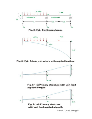
6. It is observed that, in the actual structure, the deflections at joints B and C is
zero. Now the total deflections at B and C of the primary structure due to applied
external loading and redundants R1 and R2 is,
Δ 1 = (Δ L )1 + a11 R1 + a12 R2 (8.4a)
Δ 2 = (Δ L )2 + a 21 R1 + a 22 R2 (8.4b)
The equation (8.4a) represents the total displacement at B and is obtained by
superposition of three terms:
1) Deflection at B due to actual load acting on the statically determinate
structure,
2) Displacement at B due to the redundant reaction R1 acting in the positive
direction at B (point 1) and
3) Displacement at B due to the redundant reaction R2 acting in the positive
direction at C .
The second equation (8.4b) similarly represents the total deflection at C . From
the physics of the problem, the compatibility condition can be written as,
Δ 1 = (Δ L )1 + a11 R1 + a12 R2 = 0 (8.5a)
Δ 2 = (Δ L )2 + a 21 R1 + a 22 R2 = 0 (8.5b)
The equation (8.5a) and (8.5b) may be written in matrix notation as follows,
⎧ (Δ L )1 ⎫ ⎡ a11 a12 ⎤ ⎧ R1 ⎫ ⎧0⎫
⎨ ⎬+ ⎨ ⎬=⎨ ⎬
(Δ L )2 ⎭ ⎢a 21 a 22 ⎥ ⎩ R2 ⎭ ⎩0⎭
(8.6a)
⎩ ⎣ ⎦
{(Δ L )1 } + [A]{R} = {0} (8.6b)
In which,
⎧( Δ ) ⎫ ⎡a a12 ⎤ ⎧ R1 ⎫
{( Δ ) } = ⎪( Δ ) ⎪ ; [ A] = ⎢a
L 1 ⎨
L 1
⎬
11
⎥ and {R} = ⎨ R ⎬
⎪
⎩ L 2 ⎪
⎭ ⎣ 21 a22 ⎦ ⎩ 2⎭
Solving the above set of algebraic equations, one could obtain the values of
redundants, R1 and R2 .
{R} = −[A]−1 {Δ L } (8.7)
Version 2 CE IIT, Kharagpur

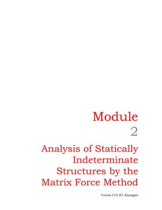
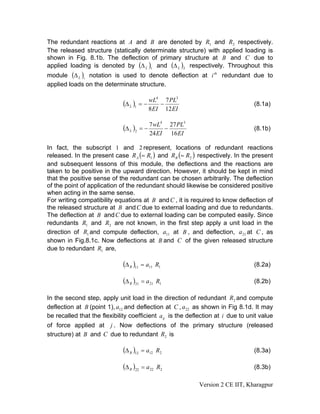
7. In the above equation the vectors {Δ L } contains the displacement values of the
primary structure at point 1 and 2, [A] is the flexibility matrix and {R} is column
vector of redundants required to be evaluated. In equation (8.7) the inverse of the
flexibility matrix is denoted by [A] . In the above example, the structure is
−1
indeterminate to second degree and the size of flexibility matrix is 2 × 2 . In
general, if the structure is redundant to a degree n , then the flexibility matrix is of
the order n × n . To demonstrate the procedure to evaluate deflection, consider
the problem given in Fig. 8.1a, with loading as given below
w=w; P = wL (8.8a)
Now, the deflection (Δ L )1 and (Δ L )2 of the released structure can be evaluated
from the equations (8.1a) and (8.1b) respectively. Then,
4
7 wL4 17 wL4
(Δ L )1 = − wL − =− (8.8b)
8 EI 12 EI 24 EI
7 wL4 27 wL4 95wL4
(Δ L )2 =− − =− (8.8c)
24 EI 16 EI 48EI
The negative sign indicates that both deflections are downwards. Hence the
vector {Δ L } is given by
wL4 ⎧34⎫
{Δ L } = − ⎨ ⎬ (8.8d)
48 EI ⎩95⎭
The flexibility matrix is determined from referring to figures 8.1c and 8.1d. Thus,
when the unit load corresponding to R1 is acting at B , the deflections are,
L3 5 L3
a11 = , a 21 = (8.8e)
3EI 6 EI
Similarly when the unit load is acting at C ,
5L3 8L3
a12 = , a 22 = (8.8f)
6 EI 3EI
The flexibility matrix can be written as,
L3 ⎡2 5 ⎤
[A] = ⎢5 16⎥ (8.8g)
6 EI ⎣ ⎦
Version 2 CE IIT, Kharagpur

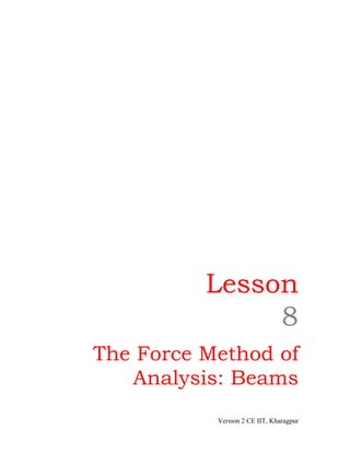
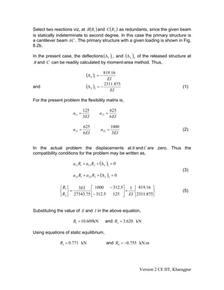
8. The inverse of the flexibility matrix can be evaluated by any of the standard
method. Thus,
16 − 5⎤
[A]−1 = 6 EI ⎡
3 ⎢ ⎥ (8.8h)
7 L ⎣− 5 2 ⎦
Now using equation (8.7) the redundants are evaluated. Thus,
⎧ R1 ⎫ 6 EI wL4 ⎡ 16 − 5⎤ ⎧34⎫
⎨ ⎬= 3 × ⎢− 5 2 ⎥ ⎨95⎬
⎩ R2 ⎭ 7 L 48 EI ⎣ ⎦⎩ ⎭
69 20
Hence, R1 = wL and R2 = wL (8.8i)
56 56
Once the redundants are evaluated, the other reaction components can be
evaluated by static equations of equilibrium.
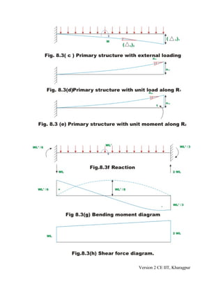
Example 8.1
Calculate the support reactions in the continuous beam ABC due to loading as
shown in Fig. 8.2a. Assume EI to be constant throughout.
Version 2 CE IIT, Kharagpur

9. Select two reactions viz, at B(R1 ) and C (R2 ) as redundants, since the given beam
is statically indeterminate to second degree. In this case the primary structure is
a cantilever beam AC . The primary structure with a given loading is shown in Fig.
8.2b.
In the present case, the deflections (Δ L )1 , and (Δ L )2 of the released structure at
B and C can be readily calculated by moment-area method. Thus,
(Δ L )1 = − 819.16
EI
and (Δ L )2 =−
2311.875
(1)
EI
For the present problem the flexibility matrix is,
125 625
a11 = a 21 =
3EI 6 EI
625 1000
a12 = a 22 = (2)
6 EI 3EI
In the actual problem the displacements at B and C are zero. Thus the
compatibility conditions for the problem may be written as,
a11 R1 + a12 R2 + (Δ L )1 = 0
(3)
a 21 R1 + a 22 R2 + (Δ L )2 = 0
⎧ R1 ⎫ 3EI ⎡ 1000 − 312.5⎤ 1 ⎧ 819.16 ⎫
⎨ ⎬= ⎢ × ⎨ ⎬
125 ⎥ EI
(5)
⎩ R2 ⎭ 27343.75 ⎣− 312.5 ⎦ ⎩2311.875⎭
Substituting the value of E and I in the above equation,
R1 = 10.609kN and R2 = 3.620 kN
Using equations of static equilibrium,
R3 = 0.771 kN and R4 = −0.755 kN.m
Version 2 CE IIT, Kharagpur

10. Example 8.2
A clamped beam AB of constant flexural rigidity is shown in Fig. 8.3a. The beam
is subjected to a uniform distributed load of w kN/m and a central concentrated
moment M = wL2 kN.m . Draw shear force and bending moment diagrams by
force method.
Select vertical reaction (R1 ) and the support moment (R2 ) at B as the
redundants. The primary structure in this case is a cantilever beam which could
be obtained by releasing the redundants R1 and R2 . The R1 is assumed to be
positive in the upward direction and R2 is assumed to be positive in the
counterclockwise direction. Now, calculate deflection at B due to only applied
loading. Let (Δ L )1 be the transverse deflection at B and (Δ L )2 be the slope at B
due to external loading. The positive directions of the selected redundants are
shown in Fig. 8.3b.
Version 2 CE IIT, Kharagpur

11. Version 2 CE IIT, Kharagpur

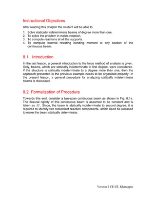
12. The deflection (Δ L )1 and (Δ L )2 of the released structure can be evaluated from
unit load method. Thus,
4
3wL4 wL4
(Δ L )1 = − wL − =− (1)
8EI 8EI 2 EI
3
wL3 2 wL3
and (Δ L )2 = − wL − =− (2)
6 EI 2 EI 3EI
The negative sign indicates that (Δ L )1 is downwards and rotation (Δ L )2 is
clockwise. Hence the vector {Δ L } is given by
wL3 ⎧3L ⎫
{Δ L } = − ⎨ ⎬ (3)
6 EI ⎩4⎭
The flexibility matrix is evaluated by first applying unit load along redundant R1
and determining the deflections a11 and a 21 corresponding to redundants R1 and
R2 respectively (see Fig. 8.3d). Thus,
L3 L2
a11 = and a 21 = (4)
3EI 2 EI
Similarly, applying unit load in the direction of redundant R2 , one could evaluate
flexibility coefficients a12 and a 22 as shown in Fig. 8.3c.
L2 L
a12 = and a 22 = (5)
2 EI EI
Now the flexibility matrix is formulated as,
L ⎡2 L2 3L ⎤
[A] = ⎢ ⎥ (6)
6 EI ⎣ 3L 6⎦
The inverse of flexibility matrix is formulated as,
Version 2 CE IIT, Kharagpur

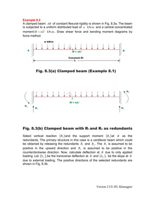
13. − 3L ⎤
[A]−1 = 6 EI ⎡
6
3 ⎢ ⎥
3L ⎣− 3L 2 L2 ⎦
The redundants are evaluated from equation (8.7). Hence,
⎧ R1 ⎫ 6 EI ⎡ 6 − 3L ⎤ ⎛ wL3 ⎞⎧3L ⎫
⎨ ⎬ =− 3 ⎢ ⎥ ×⎜− ⎟⎨ ⎬
⎩ R2 ⎭ 3L ⎣− 3L 2 L2 ⎦ ⎜ 6 EI ⎟⎩ 4 ⎭
⎝ ⎠
w ⎧ 6L ⎫
= ⎨ ⎬
3 ⎩− L2 ⎭
wL2
R1 = 2wL and R2 = − (7)
3
The other two reactions ( R3 and R4 ) can be evaluated by equations of statics.
Thus,
wL2
R4 = M A = − and R1 = R A = − wL (8)
6
The bending moment and shear force diagrams are shown in Fig. 8.3g and
Fig.8.3h respectively.
Summary
In this lesson, statically indeterminate beams of degree more than one is solved
systematically using flexibility matrix method. Towards this end matrix notation is
adopted. Few illustrative examples are solved to illustrate the procedure. After
analyzing the continuous beam, reactions are calculated and bending moment
diagrams are drawn.
Version 2 CE IIT, Kharagpur