Ab31169180

Priyanka M. Patel, V. H. Pradhan / International Journal of Engineering Research and
Applications (IJERA) ISSN: 2248-9622 www.ijera.com
Vol. 3, Issue 1, January -February 2013, pp.169-180
Travelling Wave Solutions of BBM and Modified BBM Equations
by Modified F-Expansion Method
Priyanka M. Patel1* and V. H. Pradhan1
Department of Applied Mathematics and Humanities,
S. V. National Institute of Technology, Surat-395007, India

Abstract
A new modified F-expansion method is ut  u x   u u x  u x x x  0 (2)
introduced to obtain the travelling wave
solutions like soliton and periodic, of Benjamin-
Consider the travelling wave solutions of eq. (2),
Bona-Mahony (BBM) equation and modified
under the transformation
BBM equation. The method is convenient,
effective and can be applied to other nonlinear u( x, t )  u( ) where   k ( x   t ) (3)
partial differential equations in the
mathematical physics. where k  0 and  are constants that do
determined later. By substituting eq. (3) into eq. (2)
Keywords : Modified F-expansion method, we obtain
Benjamin-Bona-Mahony (BBM) equation,
modified BBM equation, travelling wave solutions. k  u '  k u '  k  u u '  k 2 u '''  0
1. Introduction  u '  u '   u u '  k u '''  0 (4)
It is well known that nonlinear partial
differential equations (NLPDEs) are widely used to Integrating eq. (4) with respect to „  ‟ and
describe many important phenomena and dynamic
considering the zero constant for integration we
processes in physics, mechanics, chemistry and
have
biology, etc. There are many methods to solve
NLPDEs such as tanh-sech method [2], homotopy u2
analysis method [14],sine-cosine method [8], (1   ) u    k u ''  0 (5)
2
G / G  expansion
'
method [4,9],differential
where prime denotes differentiation with respect to
transform method [7], and so on. In this paper, we
apply the modified F-expansion method [3,9,10] to  . By balancing the order of u 2 and u '' in eq. (5),
the generalized BBM equation we have 2 n  n  2 then n  2
So we can see its exact solutions in the form
ut  ux   u N ux  ux x x  0 with N  1 (1)
u ( )  a0  a2 F 2 ( )  a1 F 1 ( )  a1 F ( )  a2 F 2 ( )
with constant parameter  . Wazwaz [2] (6)
has obtained the analytical solution of eq.(1) with
tanh-sech method and sine-cosine method.
Abbasbandy [14] has applied homotopy analysis where a 0 , a1 , a2 , a1 , a 2 are constants to be
method (HAM) to obtain the analytical solution of determined later. And F ( ) satisfies the
generalized BBM equation for N  1 and N  2 . following Riccati equation
In the present paper we have applied modified F-
expansion method to solve eq.(1) for N  1 and F ' ( )  A  B F ( )  C F 2 ( ) (7)
N  2 . A set of new solutions are obtained other
than the solutions obtained by previous authors.
where A , B , C are constants. Substituting eq. (6)
*Corresponding author- Email address :
pinu7986@gmail.com into eq. (5) and using eq. (7), the left-hand side of
eq. (5) can be converted into a finite series in
2. Travelling wave solutions of BBM F p ( ) , ( p = -4, -3 ,-2, -1, 0, 1, 2, 3, 4).
equation Equating each coefficient of F ( ) to zero yields
p
For N  1, eq.(1) reduces to the BBM equation or
the following set of algebraic equations.
the regularized long-wave equation (RLW).

169 | P a g e

a2 
F 4 ( ) : (12 A2 k  a2 ) 
2

F 3 ( ) : 2 A2 ka1  10 ABka2  a1a2 

a 
2

F 2 ( ) : Ak (3Ba1  8Ca2 )  1  a2 (1  4 B 2 k    a0 )
2 
F ( ) : a1 (1  B k  2 ACk    a0 )  a2 (6 BCk  a1 )
1 2 

a
2 

F 0 ( ) : a0  BCka1  2C 2 ka2  ABka1  2 A2 ka2  a0  0  a1a1  a2 a2  (8)
2 
F ( ) : a1 (1  B k  2 ACk    a0 )  a2 (6 ABk  a1 )
1 2


a12 
F ( ) : 3BCka1  4 B ka2 
2 2
 a1 (1  8 ACk    a0 )
2 

F ( ) : 2C ka1  10 BCka2  a1a2
3 2

1 
F 4 ( ) : a2 (12C 2 k  a2 ) 
2 

Solving the above algebraic equations by symbolic computations , we have the following solutions:
Case 1: A  0 , we have
12BCk 12C 2 k
a0  a0 , a1  0 , a2  0 , a1  , a2  ,   1  B 2 k  a0 (9)
 
Case 2: B  0 , we have
12C 2 k 
a0  a0 , a1  0, a2  0, a1  0, a2  ,   1  8 ACk  a0 
 
 (10)
12 A k
2
12C k2
a0  a0 , a1  0, a2  , a1  0, a2  ,   1  8 ACk  a0 
  

So we can list the solutions of u as follows:
When A  0, B  1, C  1 , from appendix and case 1, we have
3k  
u1 ( )  a0  sec h 2   (11)
 2
where   k ( x  (1  k  a0 ) t )
When A  0, B  1, C  1 , from appendix and case 1, we have
3k  
u2 ( )  a0  csc h 2   (12)
 2
where   k ( x  (1  k  a0 ) t )
1 1
When A  , B  0, C   , from appendix and case 2, we have
2 2
3k
u3 ( )  a0  coth( )  csc h( )
2
(13)

3k 3k
coth( )  csc h( ) coth( )  csc h( ) 
2
u4 ( )  a0  
2
(14)
 
3k
u5 ( )  a0   tanh( )  i sec h( )
2
(15)


170 | P a g e

3k 3k
 tanh( )  i sec h( )  tanh( )  i sec h( )
2
u6 ( )  a0  
2
(16)
 
where   k  x  1  2k  a0  t 
12k
u7 ( )  a0  tanh 2   (17)

12k 12k
u8 ( )  a0  tanh 2    tanh 2   (18)
 
12k
u9 ( )  a0  coth 2   (19)

12k 12k
u10 ( )  a0  coth 2    coth 2   (20)
 
where   k ( x  (1  8k  a0 ) t )
1 1
When A  , B  0, C  , from appendix and case 2, we have
2 2
3k
u11    a0  sec    tan  
2

   (21)

3k 2 3k
u12    a0  sec    tan    sec    tan  
2

      (22)

3k
u13    a0  csc    cot   
2

   (23)

3k 2 3k
u14    a0  csc    cot    csc    cot  
2

      (24)

where   k  x  (1  2k  a0 ) t 
1 1
When A   , B  0, C   , from appendix and case 2, we have
2 2
3k
u15    a0  sec    tan  
2

   (25)

3k 2 3k
u16    a0  sec    tan     sec    tan  
2

      (26)

3k
u17    a0  csc    cot  
2

   (27)

3k 2 3k
u18    a0  csc    cot     csc    cot  
2

      (28)

where   k  x  (1  2k  a0 ) t 
When A  1  1 , B  0, C  1 1 , from appendix and case 2, we have
12k
u19    a0  tan 2   (29)

12k 12k
u20    a0  tan 2    tan 2   (30)
 
12k
u21    a0  cot 2   (31)


171 | P a g e

12k 12k
u22    a0  cot 2    cot 2   (32)
 
where   k  x  1  8k  a0  t 

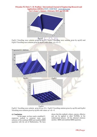
2.1 Discussion shape and propagates at constant speed. It is a
Travelling wave solutions from eq.(11) to stable solution. The first observation of this kind of
eq.(20) represents the soliton solutions and from wave was made in 1834 by John Scott Russell [5].
eq. (21) to eq.(32) represents the periodic If we draw the solution with a constant speed, we
solutions. will get the following figure (A.1) which shows the
We discuss one travelling wave solution given by right moving wave at different values of t .
eq. (11). The travelling wave solution (11) is a
solitary like solution which does not change its

4
t=0
t=1
t=2
3.5
t=3

3

2.5
u

2

1.5

1
-10 -8 -6 -4 -2 0 2 4 6 8 10
x

Fig. A.1. Plot of travelling wave solution eq. (11) with k    a0  1 and t  0,1, 2,3

If we draw the travelling wave solution spread out. If we take negative values of  (
(11) with different positive values of  (   1,  1.5,  2 ), we will get the following
  1,1.5, 2 ), we will get the following figure figure (A.2-II) which shows the value of negative
(A.2-I) which shows the value of positive amplitude. Here negative amplitude means the
amplitude in decreasing. In other words the value wave is going to look upside down. From figures
of positive amplitude tends to zero. From this (A.2-I) and (A.2-II) we can say that positive and
physically we can say that the fluid becomes more negative amplitudes are the same
.
4 1
alpha=1
alpha=1.5 alpha= -1
alpha=2 alpha= -1.5
3.5 0.5
alpha= -2

3 0

2.5 -0.5
u

u

2 -1

1.5 -1.5

1 -2
-10 -8 -6 -4 -2 0 2 4 6 8 10 -10 -8 -6 -4 -2 0 2 4 6 8 10
x x

(I) (II)
Fig. A.2. Different solitary waves profiles given by eq. (11) at t  0 , a0  k  1 for (I)   1,1.5,2 and (II)
  1,  1.5,  2

172 | P a g e

If we draw the travelling wave solution (11) with amplitude in increasing. The amplitude is
different values of k ( k  1, 2,3 ), we will get the proportional to the velocity, which means that
following figure (A.3) which describes the value of larger pulse travel faster than smaller ones.

10
k=1
9 k=2
k=3
8

7

6
u

5

4

3

2

1
-10 -8 -6 -4 -2 0 2 4 6 8 10
x

Fig. A.3. Different solitary waves profiles given by eq. (11) at t  1 , a0    1 for k  1, 2,3
The other solitary and periodic solutions are graphically shown in fig.(A.4) to fig.(A.10).

Solitary solutions

Fig.A.4 Fig.A.5
Fig.A.4. Travelling wave solution given by eq. (17) with values a0    k  1 and Fig.A.5. Travelling wave
solution given by eq.(14) with values a0  2 and   k 1

Fig.A.6
Fig.A.6 Travelling wave solution given by absolute of eq. (15) with values a0  2 and   k  1

173 | P a g e

Trigonometric solutions :

Fig.A.7 Fig.A.8
Fig.A.7. Travelling wave solution given by eq. (23) and Fig.A.8 travelling wave solution given by eq.(25) with
values a0    k  1

Fig.A.9 Fig.A.10
Fig.A.9. Travelling wave solution given by eq. (29) and Fig.A.10. Travelling wave solution given by eq.(31)
with values a0    k  1

3. Travelling wave solutions of modified BBM equation
For N  2 , eq.(1) reduces to the modified BBM equation.
ut  ux   u 2 ux  ux x x  0 (33)
Now, we construct the travelling wave solutions of eq. (33), under the transformation
v  x, t   v   where   k  x   t  (34)
where k  0 and  are constants. Substituting eq. (34) into the eq. (33), we get
k  v '  k v '   k v 2 v '  k 3 v '''  0 (35)
Integrating eq. (35) with respect to „  ‟ and considering the zero constant for integration we have

1    v  v3  k 2v''  0 (36)
3
where prime denotes differentiation with respect to  . By balancing the order of v and v in eq. (36), we have
3 ''

3 m  m  2 then m  1. So we can write
v    a0  a1 F 1    a1 F   (37)
where a 0 , a1 , a1 are constants to be determined later. And F ( ) satisfies Riccati equation given by eq. (7).
Substituting eq. (37) into eq. (36) and using eq. (7), the left-hand side of eq. (36) can be converted into a finite

174 | P a g e

series in F ( ) , ( p = -3 ,-2,-1, 0, 1, 2, 3). Equating each coefficient of F ( ) to zero yields the following
p p

set of algebraic equations.
a13 
F 3   : 2 A2 k 2 a1  
3 
F   : 3 ABk a1  a0 a12
2 2


F 1   : a1  B 2 k 2 a1  2 ACk 2 a1  a1  a0 2 a1  a12 a1 

a03 
F   : a0  BCk a1  ABk a1  a0 
0 2 2
 2a0 a1a1  (38)
3 
F 1   : a1  B 2 k 2 a1  2 ACk 2 a1  a1  a0 2 a1  a1a12 

F 2   : 3BCk 2 a1  a0 a12 

a1 
3

F   : 2C k a1 
3 2 2

3 

Solving the algebraic equations above by symbolic computations, we have the following solutions:

Case 3: A  0 , we have
3 6 B2k 2
a0   i B k , a1  0 , a1   i C k ,   1  (39)
2  2
Case 4: B  0 , we have
6 
a0  0, a1  0, a1   i C k ,   1  2 ACk 2 
 
 (40)
6 6 2
a0  0, a1   i A k , a  iC k ,   1  4 ACk 
 1  
So we can list the solutions of v as follows:
3  
v1 ( )   i k tanh   (41)
2 2
  k2  
where   k  x   1  t 
  2 
When A  0, B  1, C  1 , from appendix and case 3, we have
3  
v2 ( )   i k coth   (42)
2 2
  k2  
where   k  x   1  t 
  2 
1 1
When A  , B  0, C   , from appendix and case 4, we have
2 2
ik 6
v3 ( )    coth( )  csc h( )  (43)
2 
ik 6
v4 ( )    tanh    i sec h   
2    (44)

175 | P a g e

  k2  
where   k  x  1  t 
  2  
ik 6 ik 6
coth( )  csc h( )  coth( )  csc h( ) 
1
v5 ( )   (45)
2  2 
ik 6 1 ik 6
v6 ( )    tanh    i sec h    
   tanh    i sec h    46)
2  2   

where 
  k x  1  k 2  t 
6
v7 ( )   i k tanh   (47)

6
v8 ( )   i k coth   (48)

where 
  k x  1  2 k 2  t 
6 6
v9 ( )  i k tanh 1    i k tanh   (49)
 
6 6
v10 ( )   i k coth 1    i k coth   (50)
 
where  
 k x  1  4 k 2  t 
1 1
When A  , B  0, C  , from appendix and case 4, we have
2 2
ik 6
v11     sec    tan   
2    (51)

ik 6
v12      csc    cot   
2    (52)

  1 2 
where   k  x  1  k  t 
  2  
ik 6 1 ik 6
v13     sec    tan    
  sec    tan   
2    (53)
2 
ik 6 1 ik 6
v14      csc    cot    
   csc    cot   
2    (54)
2 
where 
  k x   1  k 2  t 
1 1
When A   , B  0, C   , from appendix and case 4, we have
2 2
ik 6
v15     sec    tan   
2    (55)

ik 6
v16      csc    cot   
2    (56)

176 | P a g e

  k2  
where   k  x  1  t 
  2 
ik 6 1 ik 6
v17     sec    tan    
  sec    tan   
2    (57)
2 
ik 6 1 ik 6
v18      csc    cot    
   csc    cot   
2    (58)
2 
where 
  k x   1  k 2  t 
When A  1  1 , B  0, C  1 1 , from appendix and case 4, we have

6
v19        i k tan   (59)

6
v20        i k cot   (60)

where 
  k x  1  2 k 2  t 
6 6
v21        i k tan 1       i k tan   (61)
 
6 6
v22        i k cot 1       i k cot   (62)
 
where 
  k x   1  4 k 2  t 
The travelling wave solutions given by eq.(41) to eq.(50) represents soliton-like solutions and eq.(51) to eq.(62)
represents periodic solutions. Some absolute of solitary and periodic solutions are shown in fig.(B.1) to
fig.(B.6).

Solitary solutions:

Fig.B.1 Fig.B.2

177 | P a g e


Fig.B.3
Fig.B.1 Travelling wave solution given by eq.(41), Fig.B.2 Travelling wave solution given by eq.(42) and
Fig.B.3 Travelling wave solution given by eq.(47) with values   k  1

Trigonometric solutions:

Fig.B.4 Fig.B.5

Fig.B.6
Fig.B.4 Travelling wave solution given by eq. (51), Fig.B.5 Travelling solution given by eq.(56) and Fig.B.6
Travelling wave solution given by eq.(60) with values   k  1

4. Conclusion shown that this method is direct, concise, effective
In this paper, we have used a modified F- and can be applied to other NLPDEs in the
expansion method to construct more exact mathematical physics. All the obtained solutions
solutions of the nonlinear BBM and modified BBM satisfies BBM and modified BBM equations.
equations with the aid of Mathematica. We have

178 | P a g e

Appendix A
Relations between values of ( A, B, C ) and corresponding F   in Riccati equation

F '    A  B F    C F 2  

A B C F  

1 1  
0 1 1  tanh  
2 2 2
1 1  
0 1 1  coth  
2 2 2
1 1
0  coth    csch   , tanh    i sec h  
2 2

1 0 1 tanh   , coth  

1 1
0 sec    tan   , csc    cot  
2 2
1 1
 0  sec    tan   , csc    cot  
2 2

1 1 0 1 1 tan   , cot  

1
0 0 0  ( m is an arbitrary constant)
C  m
arbitrary
constant 0 0 A

arbitrary exp  B   A
constant 0 0
B

References
[1]. A.I.Volpert, Vitaly A. Volpert, Vladimir [5]. J-H. He, “Soliton perturbation”,Selected
A. Volpert, “Travelling wave solutions of works of J-H.He, (2009), pp. 8453-8457.
parabolic systems”, American [6]. M.D.Abdur Rab, A.S.Mia, T.Akter,
Mathematical Society, (1993). “Some travelling wave solutions of Kdv-
[2]. A.Wazwaz, “New travelling wave Burger equation”, International Journal of
solutions of different physical structures to Mathematical Analysis, (2012), pp.1053-
generalized BBM equation”, Elsevier, 1060.
(2006), pp.358-362. [7]. M.T.Alquran, “Applying differential
[3]. G.Cai, Q.Wang, “A modified F-expansion transform method to nonlinear partial
method for solving nonlinear PDEs”, differential equations: A modified
Journal of Information and Computing approach”, Applications and Applied
Science”, (2007), pp.03-16. Mathematics:An International Journal,
[4]. J.Manafianheris, “Exact solutions of the (2012), pp.155-163.
BBM and MBBM equations by the [8]. M.T.Alquran, “Solitons and periodic
generalized (G‟/G)-expansion method”, solutions to nonlinear partial differential
International Journal of Genetic equations by the Sine-Cosine method”,
Engineering, (2012), pp.28-32. Applied Mathematics & Information

179 | P a g e

Sciences: An International Journal, [12]. N.Taghizadeh, M.Mirzazadeh, “The
(2012), pp.85-88. modified extended tanh method with the
[9]. M.T.Darvishi, Maliheh Najafi, Riccati equation for solving nonlinear
Mohammad Najafi, “Travelling wave partial differential equations”,
solutions for the (3+1)-dimensional Mathematica Aeterna, vol.2, (2012),
breaking soliton equation by (G‟/G)- pp.145-153.
expansion method and modified F- [13]. P.G.Estevez, S.Kuru, J.Negro and
expansion method”, International Journal L.M.Nieto, “Travelling wave solutions of
of Computational and Mathematical the generalized Benjamin-Bona-Mahony
Sciences 6:2, (2012), pp.64-69.
equation”, Cornell University Library,
[10]. M.T.Darvishi, Maliheh Najafi,
Mohammad Najafi, “Travelling wave (2007), pp.1-19.
solutions for foam drainage equation by [14]. S.Abbasbandy, “Homotopy analysis
modified F-expansion method”, Food and method for generalized Benjamin-Bona-
Public health, (2012), pp. 6-10. Mahony equation”, ZAMP, (2008), pp.51-
[11]. M.Wadati, “Introduction to solitons”, 62.
Pramana Journal of Physics, (2001),
pp.841-847.

180 | P a g e

Ab31169180

More Related Content

What's hot

Viewers also liked

Similar to Ab31169180

Ab31169180