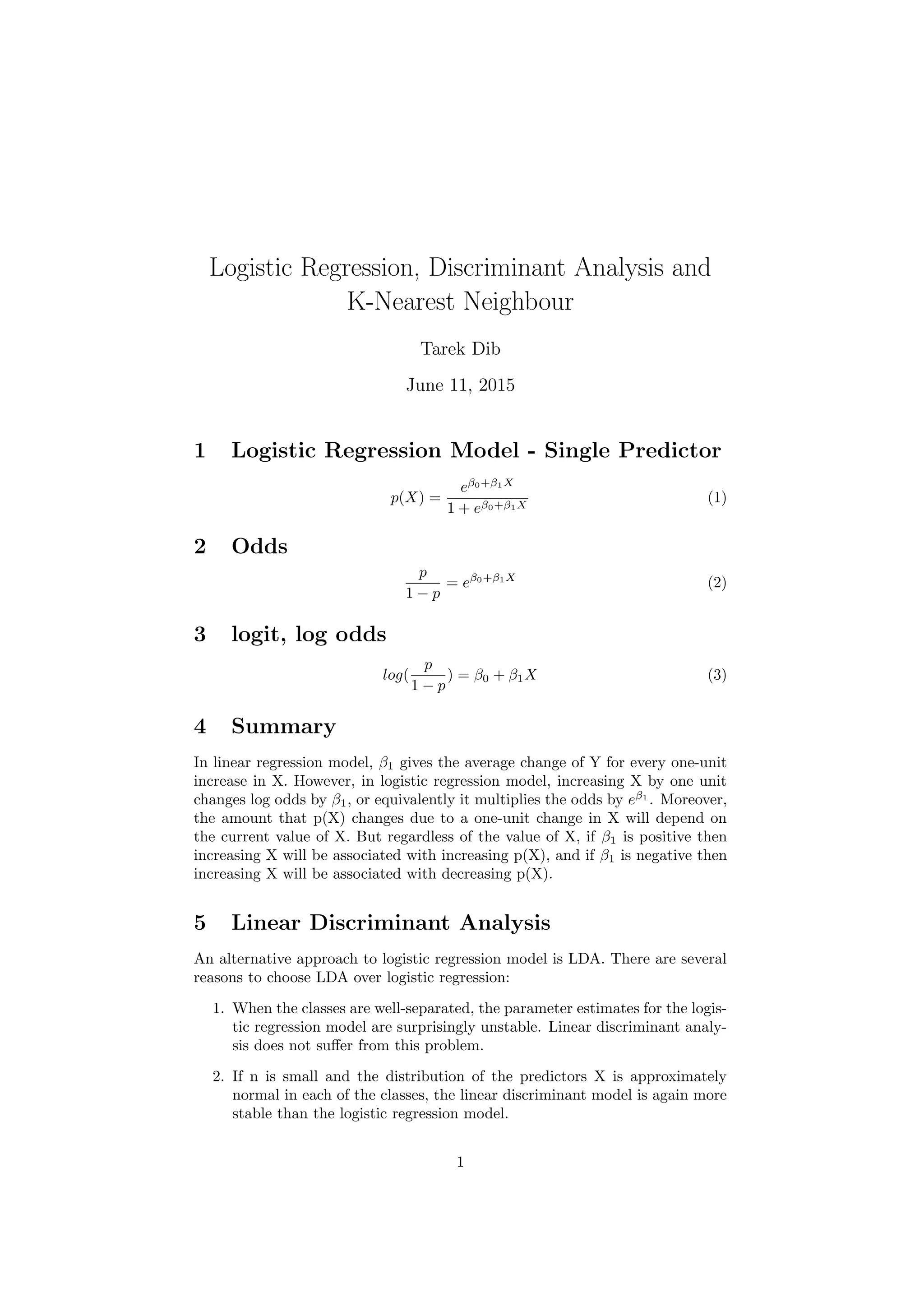
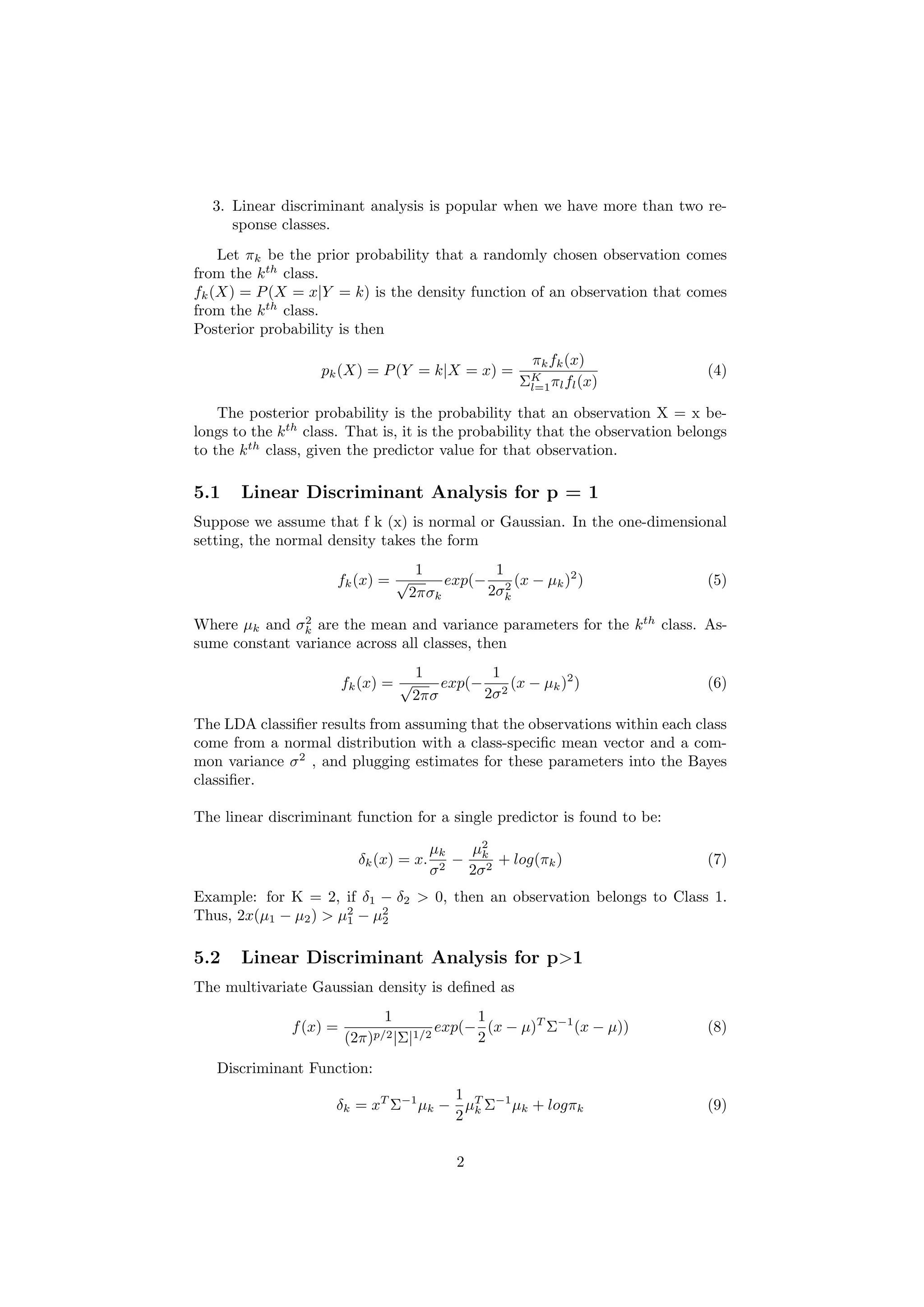
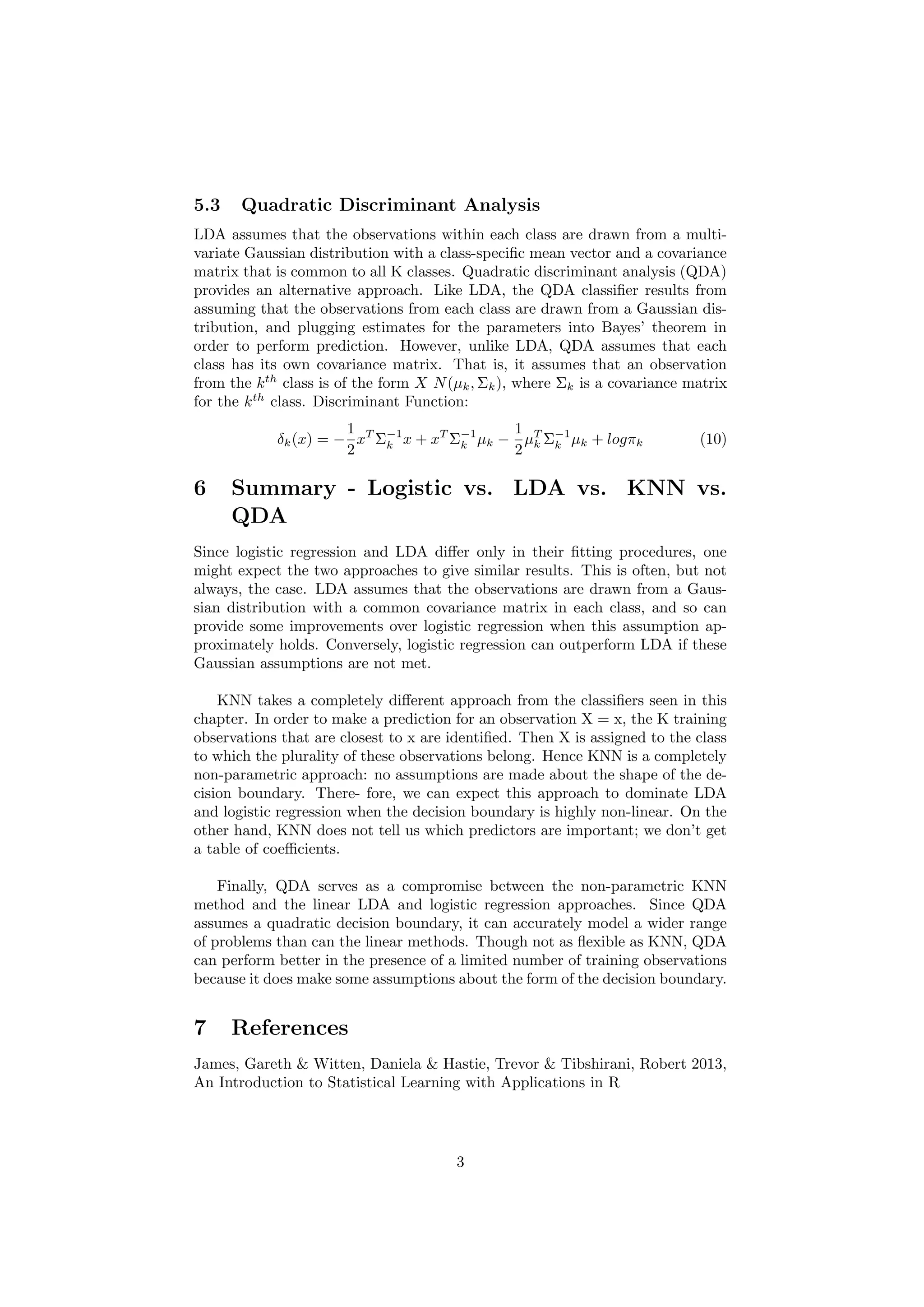
The document discusses logistic regression, linear discriminant analysis (LDA), and quadratic discriminant analysis (QDA), highlighting their applications and differences. Logistic regression models the probability of a binary outcome, while LDA is preferred when classes are well-separated and normally distributed. K-nearest neighbors (KNN) offers a non-parametric alternative that identifies the class of an observation based on the majority of its closest training examples, and QDA provides a flexible approach assuming a quadratic decision boundary.

1. Logistic Regression, Discriminant Analysis and
K-Nearest Neighbour
Tarek Dib
June 11, 2015
1 Logistic Regression Model - Single Predictor
p(X) =
eβ0+β1X
1 + eβ0+β1X
(1)
2 Odds
p
1 − p
= eβ0+β1X
(2)
3 logit, log odds
log(
p
1 − p
) = β0 + β1X (3)
4 Summary
In linear regression model, β1 gives the average change of Y for every one-unit
increase in X. However, in logistic regression model, increasing X by one unit
changes log odds by β1, or equivalently it multiplies the odds by eβ1
. Moreover,
the amount that p(X) changes due to a one-unit change in X will depend on
the current value of X. But regardless of the value of X, if β1 is positive then
increasing X will be associated with increasing p(X), and if β1 is negative then
increasing X will be associated with decreasing p(X).
5 Linear Discriminant Analysis
An alternative approach to logistic regression model is LDA. There are several
reasons to choose LDA over logistic regression:
1. When the classes are well-separated, the parameter estimates for the logis-
tic regression model are surprisingly unstable. Linear discriminant analy-
sis does not suffer from this problem.
2. If n is small and the distribution of the predictors X is approximately
normal in each of the classes, the linear discriminant model is again more
stable than the logistic regression model.
1

2. 3. Linear discriminant analysis is popular when we have more than two re-
sponse classes.
Let πk be the prior probability that a randomly chosen observation comes
from the kth
class.
fk(X) = P(X = x|Y = k) is the density function of an observation that
comes from the kth
class.
Posterior probability is then
pk(X) = P(Y = k|X = x) =
πkfk(x)
ΣK
l=1πlfl(x)
(4)
The posterior probability is the probability that an observation X = x be-
longs to the kth
class. That is, it is the probability that the observation belongs
to the kth
class, given the predictor value for that observation.
5.1 Linear Discriminant Analysis for p = 1
Suppose we assume that f k (x) is normal or Gaussian. In the one-dimensional
setting, the normal density takes the form
fk(x) =
1
√
2πσk
exp(−
1
2σ2
k
(x − µk)2
) (5)
Where µk and σ2
k are the mean and variance parameters for the kth
class. As-
sume constant variance across all classes, then
fk(x) =
1
√
2πσ
exp(−
1
2σ2
(x − µk)2
) (6)
The LDA classifier results from assuming that the observations within each class
come from a normal distribution with a class-specific mean vector and a com-
mon variance σ2
, and plugging estimates for these parameters into the Bayes
classifier.
The linear discriminant function for a single predictor is found to be:
δk(x) = x.
µk
σ2
−
µ2
k
2σ2
+ log(πk) (7)
Example: for K = 2, if δ1 − δ2 > 0, then an observation belongs to Class 1.
Thus, 2x(µ1 − µ2) > µ2
1 − µ2
2
5.2 Linear Discriminant Analysis for p>1
The multivariate Gaussian density is defined as
f(x) =
1
(2π)p/2|Σ|1/2
exp(−
1
2
(x − µ)T
Σ−1
(x − µ)) (8)
Discriminant Function:
δk = xT
Σ−1
µk −
1
2
µT
k Σ−1
µk + logπk (9)
2

3. 5.3 Quadratic Discriminant Analysis
LDA assumes that the observations within each class are drawn from a multi-
variate Gaussian distribution with a class-specific mean vector and a covariance
matrix that is common to all K classes. Quadratic discriminant analysis (QDA)
provides an alternative approach. Like LDA, the QDA classifier results from
assuming that the observations from each class are drawn from a Gaussian dis-
tribution, and plugging estimates for the parameters into Bayes’ theorem in
order to perform prediction. However, unlike LDA, QDA assumes that each
class has its own covariance matrix. That is, it assumes that an observation
from the kth
class is of the form X ∼ N(µk, Σk), where Σk is a covariance
matrix for the kth
class. Discriminant Function:
δk(x) = −
1
2
xT
Σ−1
k x + xT
Σ−1
k µk −
1
2
µT
k Σ−1
k µk + logπk (10)
6 Summary - Logistic vs. LDA vs. KNN vs.
QDA
Since logistic regression and LDA differ only in their fitting procedures, one
might expect the two approaches to give similar results. This is often, but not
always, the case. LDA assumes that the observations are drawn from a Gaus-
sian distribution with a common covariance matrix in each class, and so can
provide some improvements over logistic regression when this assumption ap-
proximately holds. Conversely, logistic regression can outperform LDA if these
Gaussian assumptions are not met.
KNN takes a completely different approach from the classifiers seen in this
chapter. In order to make a prediction for an observation X = x, the K training
observations that are closest to x are identified. Then X is assigned to the class
to which the plurality of these observations belong. Hence KNN is a completely
non-parametric approach: no assumptions are made about the shape of the de-
cision boundary. There- fore, we can expect this approach to dominate LDA
and logistic regression when the decision boundary is highly non-linear. On the
other hand, KNN does not tell us which predictors are important; we don’t get
a table of coefficients.
Finally, QDA serves as a compromise between the non-parametric KNN
method and the linear LDA and logistic regression approaches. Since QDA
assumes a quadratic decision boundary, it can accurately model a wider range
of problems than can the linear methods. Though not as flexible as KNN, QDA
can perform better in the presence of a limited number of training observations
because it does make some assumptions about the form of the decision boundary.
7 References
James, Gareth & Witten, Daniela & Hastie, Trevor & Tibshirani, Robert 2013,
An Introduction to Statistical Learning with Applications in R
3