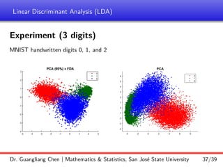
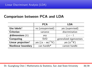
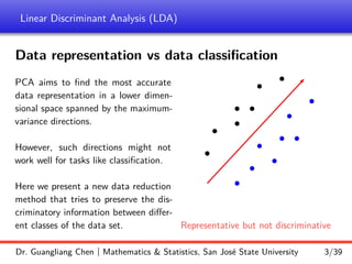
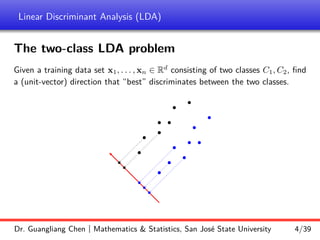
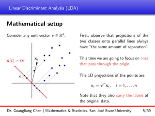
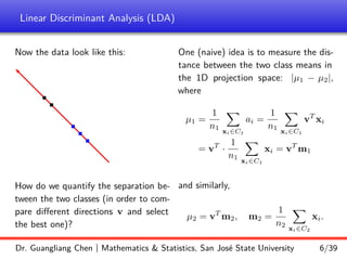
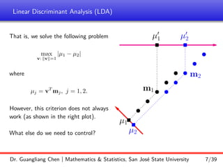
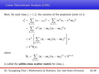
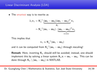
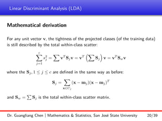
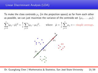
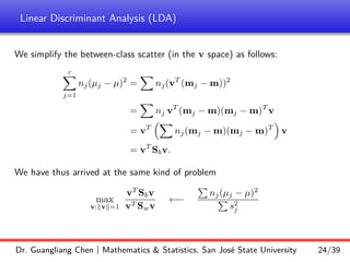
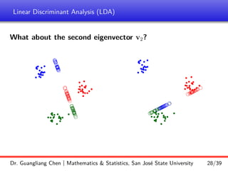
Linear discriminant analysis (LDA) is a supervised dimensionality reduction technique that aims to preserve class discriminatory information. LDA finds the optimal projection direction that maximizes separation between class means while minimizing variance within classes. For two-class LDA, the optimal direction is the solution to maximizing the ratio of between-class scatter to within-class scatter. This direction can be computed as the eigenvector corresponding to the largest eigenvalue of the matrix Sw^-1Sb, where Sw is the within-class scatter matrix and Sb is the between-class scatter matrix. Multiclass LDA generalizes this approach by maximizing the variance of the weighted class centroid means.


![Linear Discriminant Analysis (LDA)
and the projection coordinates are
Y = [0.2928, 0.0252, 0.2619, −1.0958, −1.3635, −1.1267]
-2 -1 0 1 2 3 4
-1
0
1
2
3
4
Dr. Guangliang Chen | Mathematics & Statistics, San José State University 17/39](https://image.slidesharecdn.com/lec11lda-240405073356-f038dd91/85/Lecture-on-linerar-discriminatory-analysis-17-320.jpg)
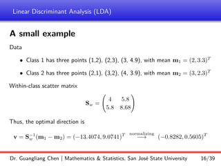
![Linear Discriminant Analysis (LDA)
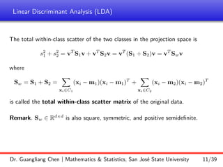
How many discriminatory directions can we find?
To answer this question, we just need to count the number of nonzero eigenvalues
S−1
w Sbv = λv
since only the nonzero eigenvectors will be used as the discriminatory directions.
In the above equation, the within-class scatter matrix Sw is assumed to be
nonsingular. However, the between-class scatter matrix Sb is of low rank:
Sb =
X
ni(mi − m)(mi − m)T
= [
√
n1(m1 − m) · · ·
√
nc(mc − m)] ·
√
n1(m1 − m)T
.
.
.
√
nc(mc − m)T
Dr. Guangliang Chen | Mathematics Statistics, San José State University 29/39](https://image.slidesharecdn.com/lec11lda-240405073356-f038dd91/85/Lecture-on-linerar-discriminatory-analysis-29-320.jpg)
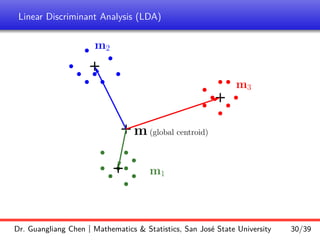
![Linear Discriminant Analysis (LDA)
Observe that the columns of the matrix
[
√
n1(m1 − m) · · ·
√
nc(mc − m)]
are linearly dependent:
√
n1 ·
√
n1(m1 − m) + · · · +
√
nc ·
√
nc(mc − m)
= (n1m1 + · · · ncmc) − (n1 + · · · + nc)m
= nm − nm
= 0.
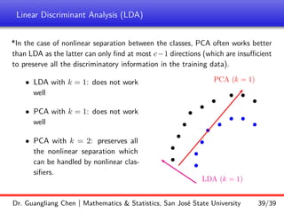
The shows that rank(Sb) ≤ c − 1 (where c is the number of training classes).
Therefore, one can only find at most c − 1 discriminatory directions.
Dr. Guangliang Chen | Mathematics Statistics, San José State University 31/39](https://image.slidesharecdn.com/lec11lda-240405073356-f038dd91/85/Lecture-on-linerar-discriminatory-analysis-31-320.jpg)
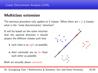
![Linear Discriminant Analysis (LDA)
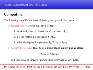
Multiclass LDA algorithm
Input: Training data X ∈ Rn×d
(with c classes)
Output: At most c − 1 discriminatory directions and projections of X onto them
1. Compute
Sw =
c
X
j=1
X
x∈Cj
(x − mj)(x − mj)T
, Sb =
c
X
j=1
nj(mj − m)(mj − m)T
.
2. Solve the generalized eigenvalue problem Sbv = λSwv to find all nonzero
eigenvectors Vk = [v1, . . . , vk] (for some k ≤ c − 1)
3. Project the data X onto them Y = X · Vk ∈ Rn×k
.
Dr. Guangliang Chen | Mathematics Statistics, San José State University 32/39](https://image.slidesharecdn.com/lec11lda-240405073356-f038dd91/85/Lecture-on-linerar-discriminatory-analysis-32-320.jpg)
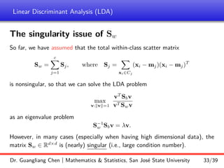
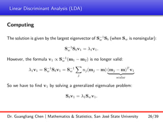
![Linear Discriminant Analysis (LDA)
How does this happen?
Let e
xi = xi−mj for each i = 1, 2 . . . , n
be the centered data points using its
own class centroid.
Define
e
X = [e
x1 . . . e
xn]T
∈ Rn×d
.
Then
Sw = e
XT e
X ∈ Rd×d
.
b
b
b
b b
b
b
b
b
b
b
b
b
b
b
b
b
b
b
b
b
b
b
b
b
+
+
+
Important issue: For high dimensional data (i.e., d is large), the centered data
often do not fully span all d dimensions, thus making rank(Sw) = rank( e
X) d
(which implies that Sw is singular).
Dr. Guangliang Chen | Mathematics Statistics, San José State University 35/39](https://image.slidesharecdn.com/lec11lda-240405073356-f038dd91/85/Lecture-on-linerar-discriminatory-analysis-35-320.jpg)
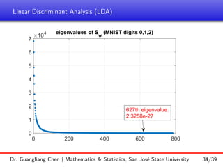
![Linear Discriminant Analysis (LDA)
Common fixes:
• Apply global PCA to reduce the dimensionality of the labeled data (all
classes)
Ypca = X − [m . . . m]T
· Vpca
and then perform LDA on the reduced data:
Zlda = Ypca · Vlda ←− learned from Ypca
• Use pseudoinverse instead: S†
wSbv = λv
• Regularize Sw:
S0
w = Sw + βId = QΛQT
+ βId = Q(Λ + βId)QT
where Λ + βId = diag(λ1 + β, . . . , λd + β).
Dr. Guangliang Chen | Mathematics Statistics, San José State University 36/39](https://image.slidesharecdn.com/lec11lda-240405073356-f038dd91/85/Lecture-on-linerar-discriminatory-analysis-36-320.jpg)