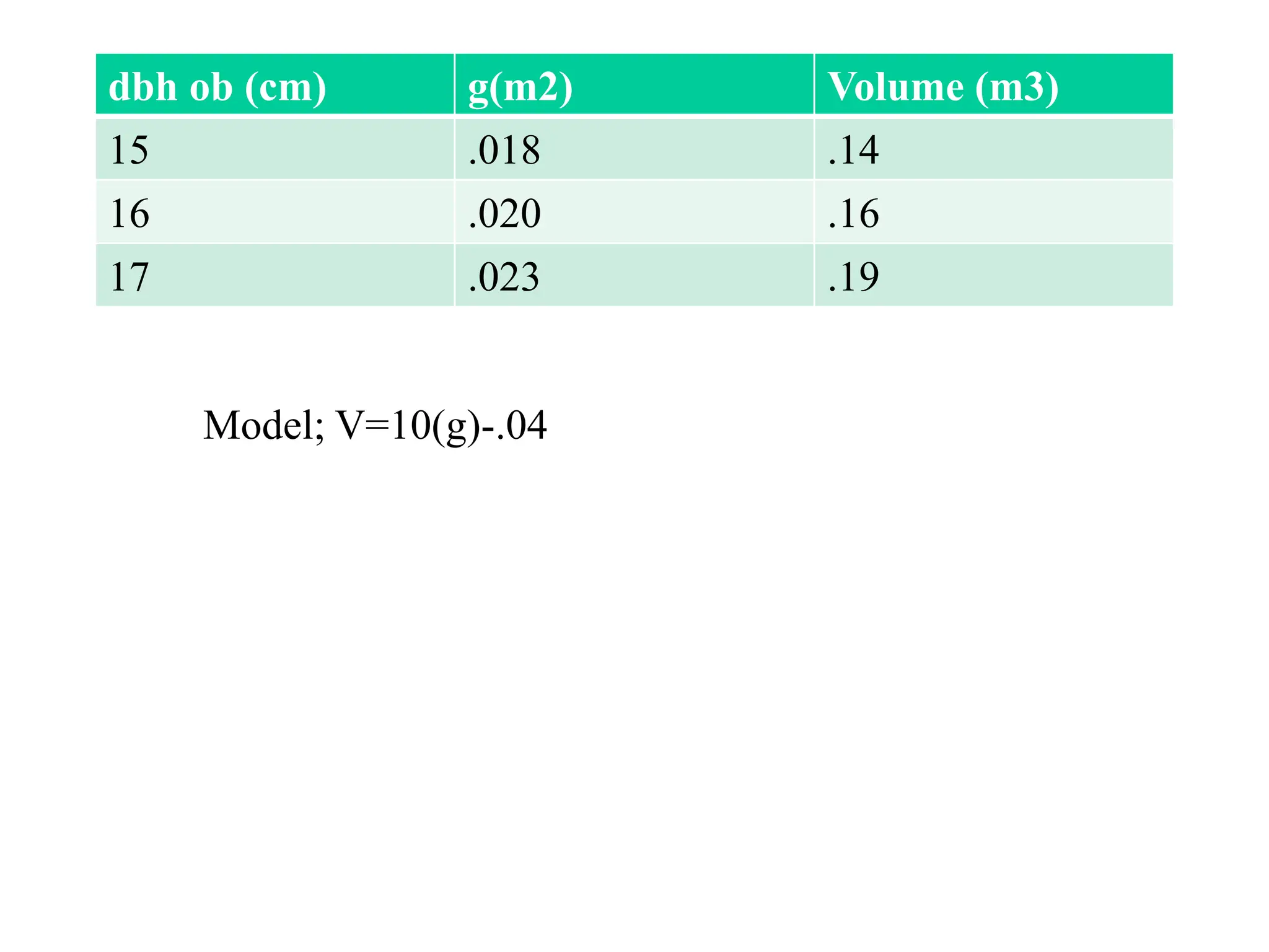
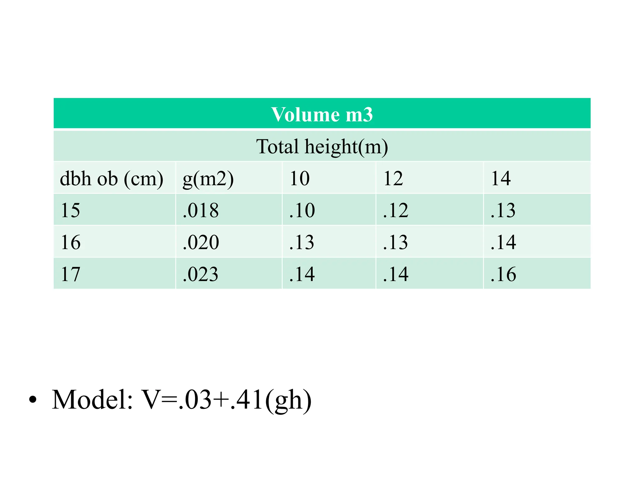
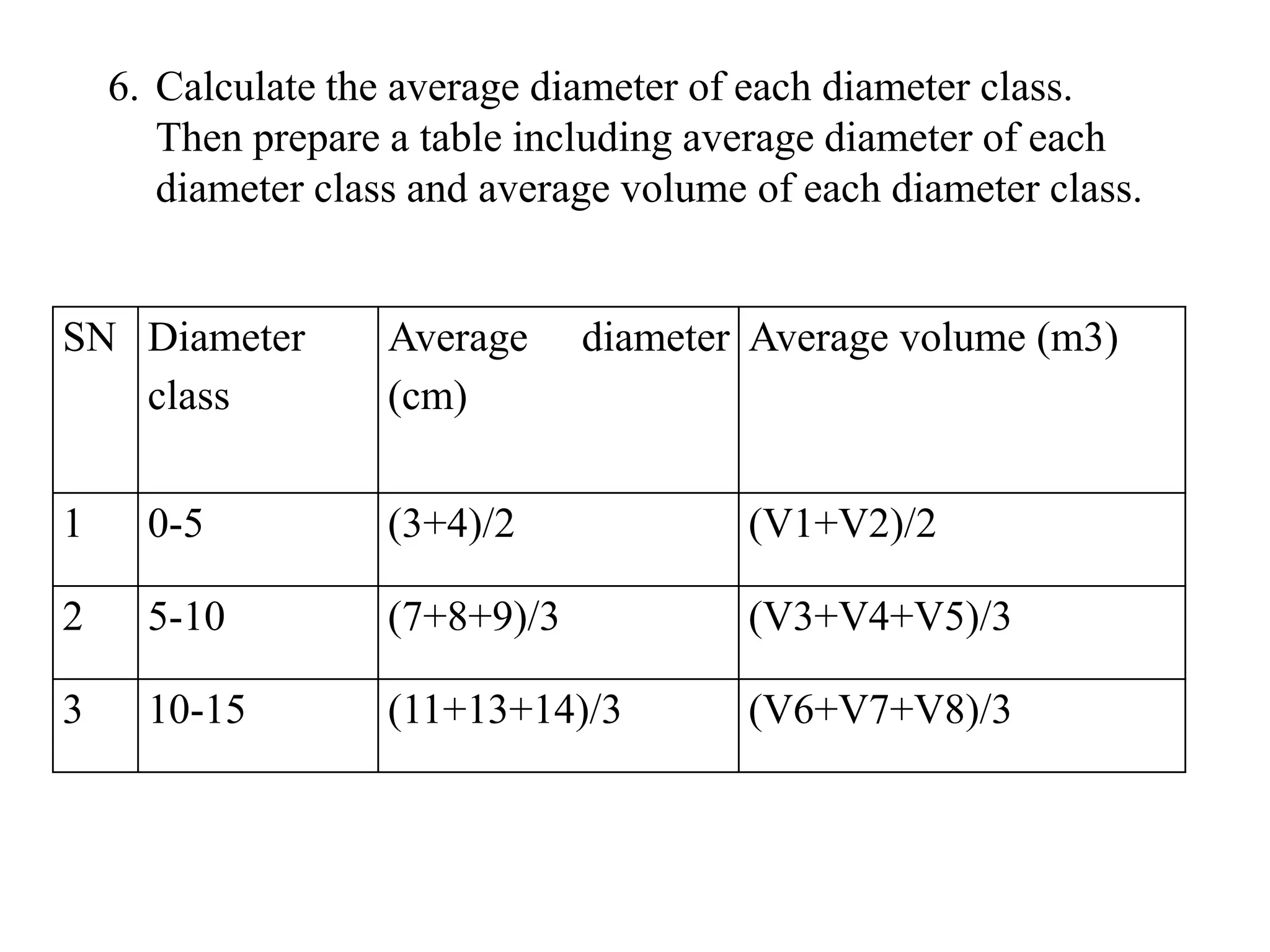
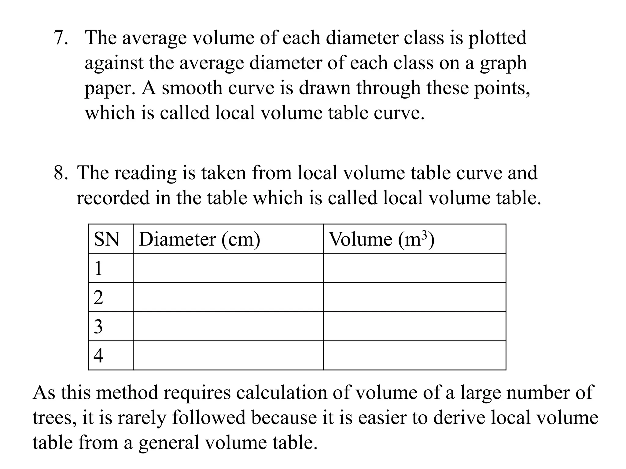
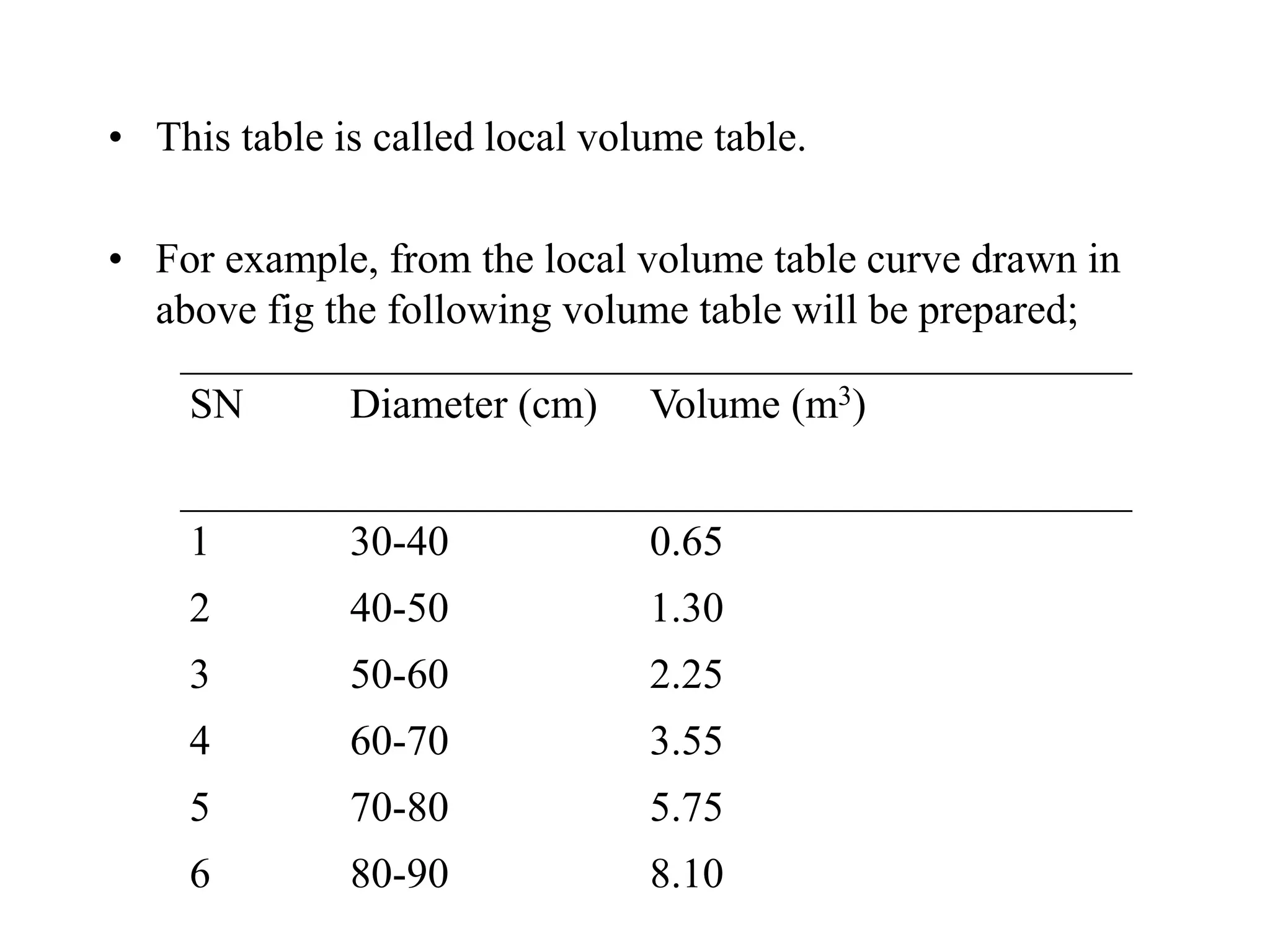
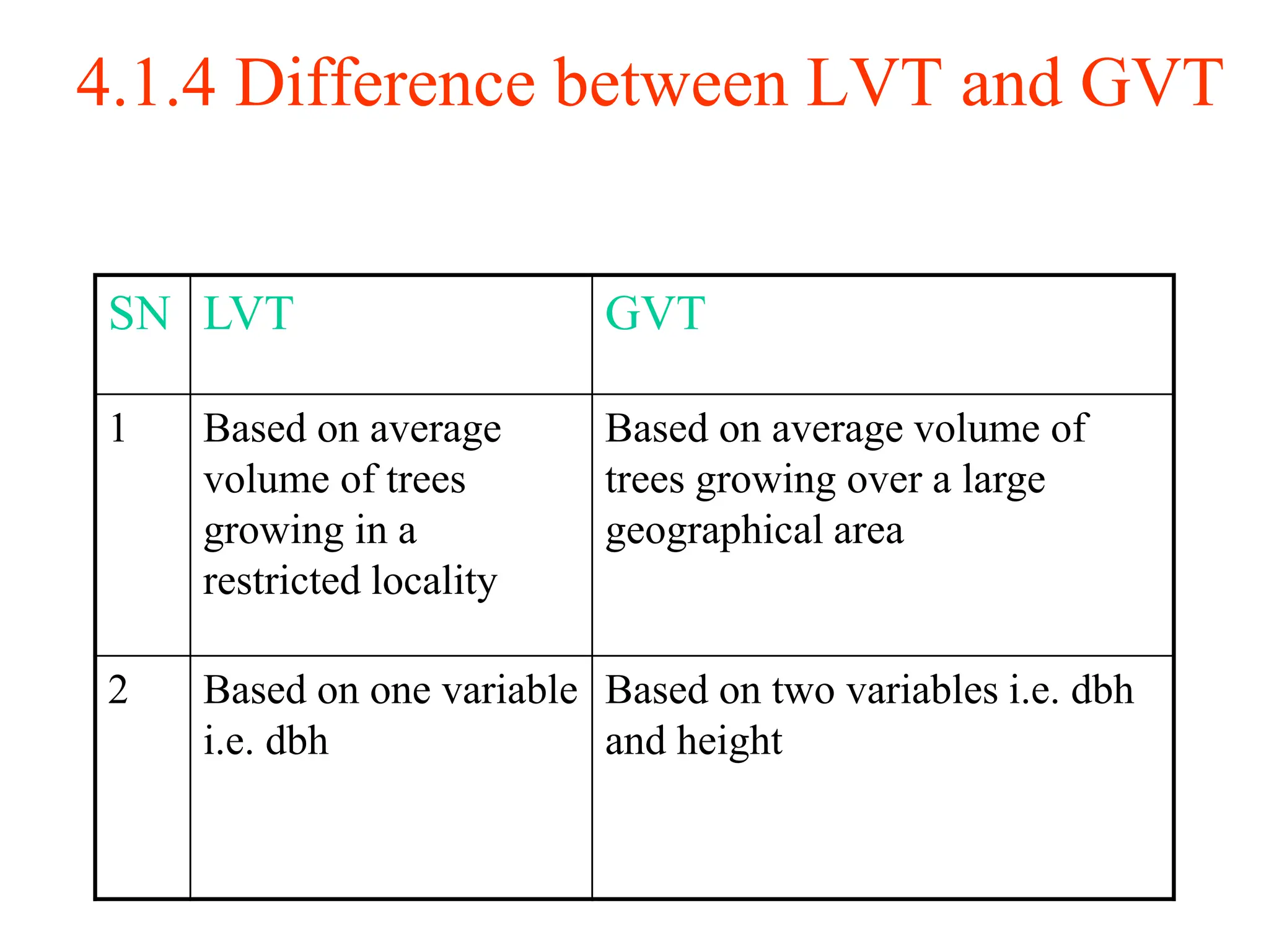
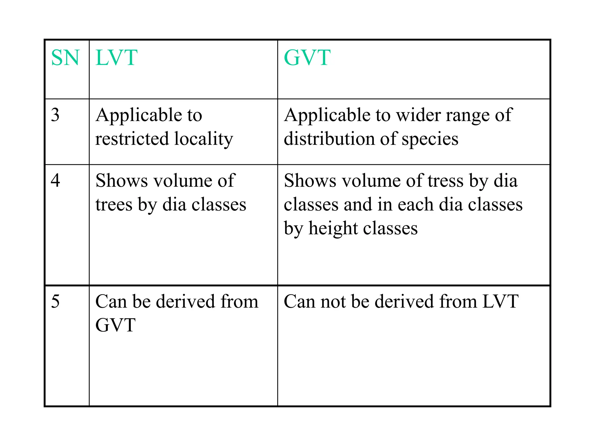
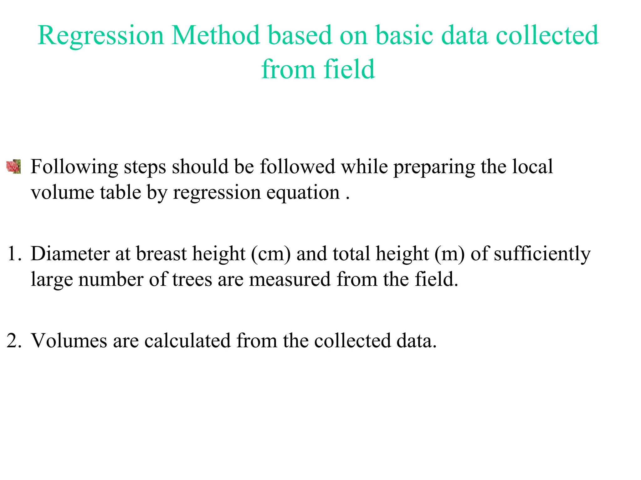
2. 4.1 Volume Tables
โข The table which shows the average contents of trees,
logs or sawn timber for one or more given dimensions
for a given species.
โข The given dimensions may be
i) dbh alone
ii) dbh and height
iii) Dbh, height and some measures of form
3. โข The object of volume table is to estimate the volume of an
average standing trees of known dimensions and thus to
estimate the volume of a given crop.
โข The volume tables are based on the actual measurement of
a large number trees and provide volume estimate of the
same species on the assumption that the trees of the same
species with same dimensions will have the same
volume.
โข Volume table can be applied only to a group of trees but
not to a individual tree.
4. What Volume Table Provides?
โข Volume
โข Name of species
โข Locality from which data were collected
โข Methods of compilation and collection
โข Applicability of the table
5. 4.1.1 Types of Volume Tables
โข Trees with identical dbh and total height, even for same
species do not necessarily have the same volume.
โข Therefore, a single universal volume table that would
apply to all conditions and species is not possible.
โข Therefore, volume tables can be classified
6. A) According to number of variable used
B) According to scope of their application
C) According to the kind of outturn given by them
7. A) Volume Tables Based on Number
of Variables Used
1) Volume Table Based on One Variable
โข Variable is dbh (ob)
โข Trees are classified by dbh only.
โข These tables show average volume of trees by dbh
classes.
8. โข Height variation in the same dbh may be frequent in
different localities, such volume tables can not be used
for extensive areas.
โข These tables can be used only locally and hence called
local volume table.
โข These tables are easy and quick to use as they require
the measurement of only dbh (ob).
9. โข The common model for this type of volume table is
V=a+b(g)
V=a1+b1(d2)
Where,
V=Volume over bark
g=basal area over bark
d=diameter at breast height over bark
a,a1,b,b1=regression constants
11. 2. Volume Tables Based on Two Variables
โข Variables are dbh and height.
โข As the trees of the same diameter may have different
heights and different volumes in different localities,
volume table based on these two variables are applicable to
larger areas.
โข These volume tables give volume of trees by dbh classes as
well as by height classes pertaining to the total height of
the tree.
12. โข Also called general volume.
โข The common model for this type of volume table is
V= a+b(d2h)
V=a+bd2+ch
Where,
V=Volume over bark
d= dbh (ob)
h= total height
a,b&c = regression constants
14. 3 Volume Tables Based on Three Variables
โข Variables are dbh, ht. and form quotient
โข Also called form class volume table
โข These volume tables are more accurate but are expensive
and difficult to construct and use and time consuming in
their application.
15. โข The common model for this type of volume is
V=a+b(d2h)+cq
Where, V=Volume of tree over bark
h=height of tree
d=diameter at breast height
q=form quotient (di/d)
di=diameter at height i above ground
a,b,c=regression constant
16. B. Volume tables based on scope of
application
1. General Volume Table
The volume table which are based on two variable i.e.
dbh and height and on the volume of trees growing over
a large geographical area.
Applicable to wider range of distribution of species.
17. Shows the volume of trees by dia classes and in each dia
classes by height classes.
Used for deriving local volume table and for estimating the
volume of trees.
Prepared from either graphical method or regression
method.
18.
19. 2. Regional Volume Table
Compiled from measurement of trees growing in a region
and limited application than general volume tables.
20. 3. Local Volume Tables
Based on one variable i.e. dbh (ob) and compiled from the
measurement of trees growing in restricted locality.
Applicable to limited locality.
These are either prepared directly from field data or
derived from general volume table, either by graphical
method or regression method.
21. C. Volume table based on kind of outturn
1. Standard Volume Tables
It gives separately the estimated outturn in the form of standard
timber, i.e. from ground level to the limit of the portion of tree
stem or branches where dia is 20 cm measured over bark, and
small wood i.e., the volume between the dia limits of 20cm and
5 cm both measured over bark.
The volume is given in terms of round timber and includes the
volume of stump.
The standard stem timber excludes the volume of bark while
standard small wood includes it.
22. 2. Commercial Volume Table
These volume tables give the contents of round timber as
volume measured down to a thin end diameter to which
conversion is done.
The stump volume is omitted.
23. 3. Sawn Outturn Tables
These volume table give the contents of sawn timber as
volume measured down to a thin end diameter to which
conversion is done.
Stump volume is omitted.
These tables are similar to commercial volume tables
except for the fact that these give volume of sawn timber
instead of volume in round.
24. 4. Assortment Volume Tables
These volume tables give the contents of round timber as
volume measured down to various stated thin end
diameters.
For example, down upto 25cm, 20cm, or 15cm diameter
limit.
The standard volume tables and commercial volume tables
are special cases of assortment tables.
25. 5. Sawn Outturn Assortment Tables
These tables are similar to assortment tables except that
they give sawn outturn in the number of standardized
pieces instead of volume in round.
26. 4.1.2 Preparation of local volume table
Local volume table can be prepared from the following two
methods.
Graphical method
Regression method
In both of the above methods, local volume tables can be
prepared either from basic data collected from field or derived
from the general volume table of that species.
27. Graphical method based on basic data collected
from the field
1. Diameter at breast height (cm) and total height (m) of sufficiently
large number of trees are measured from the field.
2. Volumes are calculated from the collected data.
28. SN Diameter (cm) Volume (m3)
1 3 V1
2 4 V2
3 7 V3
4 8 V4
5 9 V5
6 11 V6
7 13 V7
8 14 V8
3. Arrange the measured diameter in an increasing order
along with its corresponding volume.
29. 4. Prepare the diameter class like 0-5, 5-10,
10-15, 15-20 etc.
SN Diameter class Diameter (cm) Volume (m3)
1 0-5 3 V1
4 V2
2 5-10 7 V3
8 V4
9 V5
3 10-15 11 V6
13 V7
14 V8
30. 5. Calculate the average volume of each
diameter class.
SN Diameter class Diameter
(cm)
Volume
(m3)
Average volume
(m3)
1 0-5 3 V1 (V1+V2)/2
4 V2
2 5-10 7 V3 (V3+V4+V5)/3
8 V4
9 V5
3 10-15 11 V6 (V6+V7+V8)/3
13 V7
14 V8
31. 6. Calculate the average diameter of each diameter class.
Then prepare a table including average diameter of each
diameter class and average volume of each diameter class.
SN Diameter
class
Average diameter
(cm)
Average volume (m3)
1 0-5 (3+4)/2 (V1+V2)/2
2 5-10 (7+8+9)/3 (V3+V4+V5)/3
3 10-15 (11+13+14)/3 (V6+V7+V8)/3
32. 7. The average volume of each diameter class is plotted
against the average diameter of each class on a graph
paper. A smooth curve is drawn through these points,
which is called local volume table curve.
8. The reading is taken from local volume table curve and
recorded in the table which is called local volume table.
SN Diameter (cm) Volume (m3)
1
2
3
4
As this method requires calculation of volume of a large number of
trees, it is rarely followed because it is easier to derive local volume
table from a general volume table.
33. Derivation of local volume table from
general volume table by graphical method
The general volume table provides the volume of a tree by
diameter and height classes.
These are generally based on data of trees collected from a
wide range of distribution.
To use general volume table it is necessary to measure dbh
and height of individual trees.
34. Local volume table is derived from a general volume table
with the help of measurement of dbh and height of some
standing trees in the locality.
The procedure of preparation of a local volume table from
general volume is as follows:
1. Diameter and height of trees of the locality for which the
local volume table is to be prepared are accurately
measured and recorded. Suppose the diameter and height
of these trees are;
35.
36. 2. The figures of general volume table are plotted on a graph
paper showing volume against the middle of diameter
classes for each height class separately.
โข Thus there will be the same number of curves as the
number of height classes and in order to distinguish them,
they should be given a number equivalent to the middle of
the height class to which it pertains.
โข For example, the general volume table of deodar (Cedrus
deodara) gives the following data for different height
classes.
37.
38. โข Thus by plotting the volumes of each height class against the
middle of diameter class interval, 5 curves will be obtained and
they will be numbered as 17m, 23m, 29m, 35m, 41m as shown
in Fig.
39.
40. 3. Diameter and height figure of field data are then plotted on the
same graph by taking the diameter along the X-axis and then
interpolating the height against these diameters in between the
height curves of general volume tables.
โข For example, the diameter of first tree is 26cm.
โข After locating the mark on diameter axis, the same ordinate is
followed up to locate 18m by simple rule of proportion.
โข The curves already drawn are for 17m and 23m.
โข The distance between the two on that ordinate is 2mm.
โข This distance represents a gap of 23-17m = 6m.
41. โข Therefore 18m point should be 2/6mm above the 17m curve.
โข Then the diameter of second tree is 37cm.
โข After locating 37cm mark on diameter axis, the same ordinate is
followed up to locate 22m point for height.
โข This point will also be between the 17m and 23m curves.
โข The distance between two curves on the 37cm ordinate is 5mm.
โข This distance represents a gap of 23m-17m = 6m.
42. โข Therefore by simple rule of proportion the 22m mark point
will be on that ordinate at 5ร5/6=4.16mm above the 17m
curve or just 0.84mm below the 23m curve.
โข Having plotted all points in this way, a smooth curve is
drawn through these points.
โข The curve so obtained is the desired local volume table
curve and represents the local relationship between
diameter and height.
โข From this curve, volume may be read at the middle of
diameter classes and tabulated to give diameter classes and
volume.
43. โข This table is called local volume table.
โข For example, from the local volume table curve drawn in
above fig the following volume table will be prepared;
SN Diameter (cm) Volume (m3)
1 30-40 0.65
2 40-50 1.30
3 50-60 2.25
4 60-70 3.55
5 70-80 5.75
6 80-90 8.10
44. 4.1.4 Difference between LVT and GVT
SN LVT GVT
1 Based on average
volume of trees
growing in a
restricted locality
Based on average volume of
trees growing over a large
geographical area
2 Based on one variable
i.e. dbh
Based on two variables i.e. dbh
and height
45. SN LVT GVT
3 Applicable to
restricted locality
Applicable to wider range of
distribution of species
4 Shows volume of
trees by dia classes
Shows volume of tress by dia
classes and in each dia classes
by height classes
5 Can be derived from
GVT
Can not be derived from LVT
46. Regression Method based on basic data collected
from field
Following steps should be followed while preparing the local
volume table by regression equation .
1. Diameter at breast height (cm) and total height (m) of sufficiently
large number of trees are measured from the field.
2. Volumes are calculated from the collected data.
47. 3. Arrange the measured diameter in an increasing order
along with its corresponding volume.
SN Diameter (cm) Volume (m3)
1 3 V1
2 4 V2
3 7 V3
4 8 V4
5 9 V5
6 11 V6
7 13 V7
8 14 V8
48. 4. Model formulation or selection
Some models
V=a+bD
V=a+bD+cD2
Where, V= Volume, D= dbh (ob), a= regression constant,
b,c=regression coefficient
5. Calculate the volume by using best selected model and
tabulate in an appropriate format which is called local
volume table.
49. Model Selection and Evaluation
There are several statistics which are used in
selection and evaluation of the models.
1) Adjusted Coefficient of Determination (R2 adj)
R2 adj.= {1-(1-R2)(n-1)}/(n-p)
Where R2= Coefficient of determination
p=Number of parameters used in regression
model
n=Total number of observations
The model which gives the largest value is better.
50. 2. Significance of Parameter Values
If the calculated value is greater than tabulated
value, the parameter is significant. Or
If the p-value is less than 0.05, the parameter is
treated as significant.
The significant is better.
51. 3. Homogeneity and distribution of the residuals
The values of the parameters are plotted on the graph
paper.
A smooth curve is drawn by representing the values.
The model which shows the minimum residuals is
considered better.
It can be measured through histogram of residuals. The
model which shows the normal distribution is
considered better.
52. 4. Root Mean Square Error
RMSE determines the accuracy of model predictions and it is
considered as one of the most important model evaluation criteria.
The model which shows the minimum root mean square error is
considered better.
RMSE= {โโ(Yi-yi)2}/n-p
Where,
Yi & yi are observed and predicted values respectively.
n=total number of observations used to fit the model
p= number of parameters
53. 5. Logical and biological consistency of the
estimated parameters
The estimated parameter such as growth pattern should
show sigmoid pattern.
The model which shows such consistent pattern, is
considered better.
54. 6. Visual examination of the fitted curves overlaid
on the scattered plots of the observed data
While plotting expected and observed data on the graph paper, the
model which shows the minimum scatteredness is considered
better.
7. Variation Inflation Factor (VIF)
VIF measures the impact of collinearity among the independent
variables in a regression model.
It expresses the degree to which collinearity among the predictors
degrades the precision of an estimate.
VIF=1/Tolerance
55. Where,
Tolerance = 1-R2
R2 is coefficient of determination.
When VIF is greater than 10, it is considered to exist collinearity
among the independent variables.
The model which shows VIF less than 10 (if possible minimum
within 10) is considered better.
8. Simplicity, Practicability and Cost Effective
59. Models R2 adj. RMSE Parameter P VIF
V1 0.851 27.381 a
b
.000
.000
V2 0.968 12.771 a
b
c
.733ns
.143 ns
.000
12.223
12.223
V3 0.872 25.389 a
b
c
0.69 ns
.000
.044
8.319
8.319
V4 0.984 8.947 a
b
.315 ns
.000
V5 0.842 0.810 a
b
.560 ns
.000
60. Models R2 adj. RMSE Parameter P VIF
V6 0.991 0.191 a
b
.000
.000
V7 0.994 0.152 a
b
c
.000
.000
.001
11.454
11.454
V8 0.978 0.299 a
b
c
.000
.000
.000
4.120
4.120
V9 0.997 0.115 a
b
c
.000
.000
.000
14.550
14.550
V10 0.997 0.113 a
b
.000
.000
61. Derivation of Regression Equation for Local
Volume Table From the Regression Equation
of the General Volume Table
Develop the relationship between diameter and height
considering all parameters and then transform the height
relation into diameter.
62. For example,
Suppose the general volume table equation is
V=a+bD2H
and the height/diameter relationship equation for any
locality is H=c+dD+eD2,
then local volume equation will be
V=a+bD2(c+dD+eD2)
63. 4.1.3 Preparation of General Volume
Table
Regression Method
1. Diameter at breast height (cm) and total height (m) of
sufficiently large number of trees are measured from the
field.
2. Volumes are calculated from the collected data.
64. 3. Arrange the measured diameter and height along with its
corresponding volume.
SN Diameter (cm) Height (m) Volume (m3)
1 D1 H1 V1
2 D2 H2 V2
3 D3 H3 V3
4 D4 H4 V4
5 D5 H5 V5
6 D6 H6 V6
7 D7 H7 V7
8 D8 H8 V8
65. 4. Model formulation and selection
Some models
V=a+bD+cH
V=a+bD2H
Where, V= Volume, D= dbh (ob), H= Tree height, a,b,c=regression
constant
5. Calculate the volume by using best selected model and tabulate in
an appropriate format which is called general volume table.
66. Volume tables for forest trees of Nepal
โข Volume tables for forest trees of Nepal have been prepared
for 21 important tree species and species groups
(miscellaneous species in Terai and miscellaneous species
in hills).
โข For each species three volume tables are presented:
โข One for the total stem volume
โข Another for the volume to 10cm top diameter and
โข Third table for the timber volume to 20cm top diameter.
โข The total volume is expressed with bark however the other
two give the timber volume without bark.
67. Volume equations used in Nepal
Total stem volume
ln(V) = a+b ln(d)+c ln (h)
Where,
V=Total stem volume with bark
d= dbh
h=height
Ln=natural logarithm
68. Stem volume to 10 cm top diameter
ln(V1/V) = a+b(d)
Where,
V1=Overbark volume of tree top (beyond 10cm dia)
V=Total stem volume overbark
d=dbh
69. Stem volume to 20 cm top diameter
ln(V2/Vt) = a+b ln(d)
Where,
V2= overbk volume between 10 and 20 cm diameter
Vt= Overbark stem volume to 10 cm top diameter.
d=dbh
70. โข To reduce the bark volume from the stem over bark
volume, the following equation has been used
ln(Pb) = a+b ln(d)
Where,
Pb = bark proportion
d= Dbh
a,b = constants
71. SN Species SN Species
1 Abies pindrow 13 Michelia champaca
2 Acacia catechu 14 Pinus roxburghii
3 Adina cordifolia 15 Pinus wallichiana
4 Albizia species 16 Quercus species
5 Alnus nepalensis 17 Schima wallichii
6 Anogeissus latifolia 18 Shorea robusta
7 Bombax ceiba 19 Terminalia alata
8 Cedrella toona 20 Trewia nudiflora
9 Dalbergia sissoo 21 Tsuga species
10 Eugenia jambolana 22 Miscellaneous in Terai
11 Hymenodictylon excelsum 23 Miscellaneous in Hills
12 Lagerstroemia parviflora
The list of species which have volume tables
72. 4.2 Biomass table and equation
4.2.1 Root, leaf, stem and branch biomass
Biomass is the weight of the vegetative matter produced per unit
area.
Thus, the wood, their branches, bark, root and leaves produced by
trees, shrubs and other vegetation are included in biomass.
Many of the products available from forests such as fodder,
compost material and firewood are quantified in terms of weight
rather than volume.
73. The parameter to be measured and the nature of the
components for which biomass estimates are to be derived
depends on the forest types.
In Nepal, the forests can be categorized in to three types
for this purpose.
i) Natural broadleaved forests with mixed species
ii) Coniferous forests both natural and plantations
iii) Broadleaved plantation of single and mixed species
74. The general methodology for determining biomass are
common to all forest types.
dbh is the recommended predictor variable. Sometimes
height is also considered.
However for species which have a very low branching
habit or species in a coppiced broadleaved natural forest,
diameter is measured at 0.3m from the ground level is a
better predictor.
It is necessary to carry out destructive sampling to
establish correlations for estimating biomass of standing
trees.
75. About 30 trees should be selected, felled and separated into
main stem, branch wood and leaves.
The main stem should be considered up to the thin end of
10 cm girth or 3.18cm dia. The rest should be included in
branch wood.
The felling should be done as close to ground level as
possible.
Separate portions should be weighted immediately after
felling. The felled wood loses moisture very fast.
77. โข Biomass table of Castonopsis indica (natural )
Green Weight in Kg
dbh
(cm)
Stem Branch Foliage
1 - 0.2 0.3
5 7 2.4 3.7
10 37.1 12.9 10.5
15 98.7 34.2 19.4
20 197.5 68.3 29.9
78. 4.2.2 Different bio-mass equations
Many forms of regression equations have been reported by
many workers.
Some equations are
B= a+bD
B=a+bD+cH
B=a+bD2H
Widely used equation is B=a+bD2H