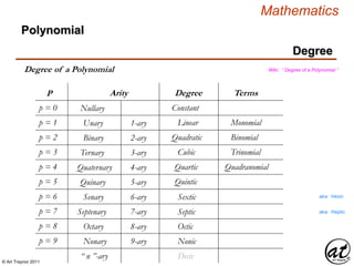
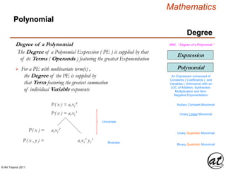
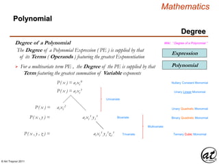
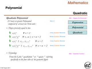
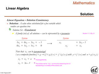
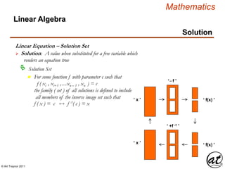
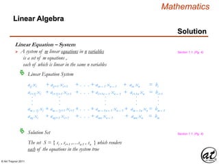
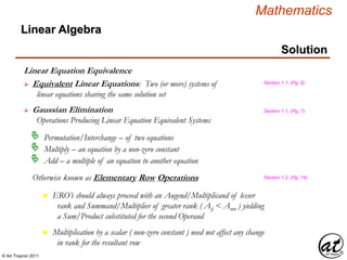
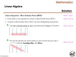
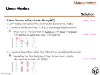
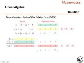
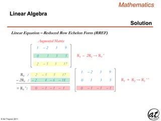
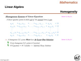
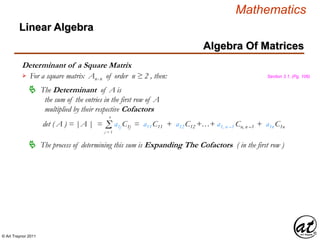
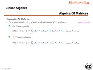
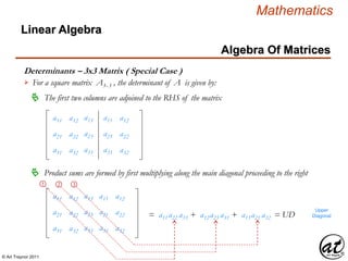
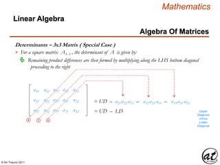
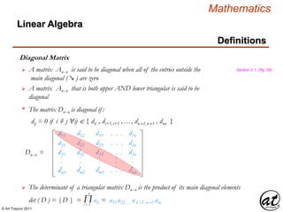
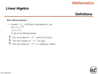
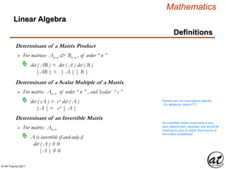
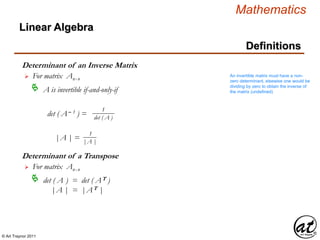
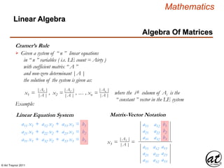
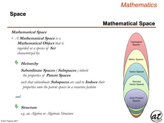
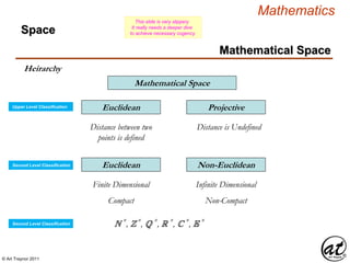
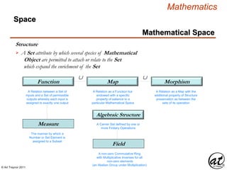
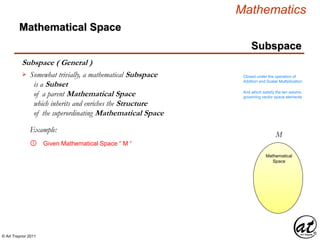
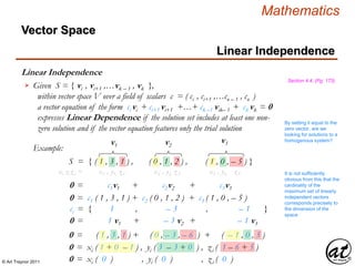
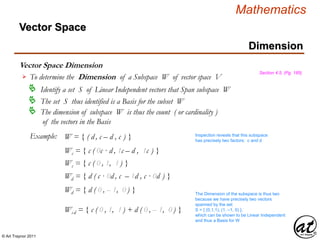
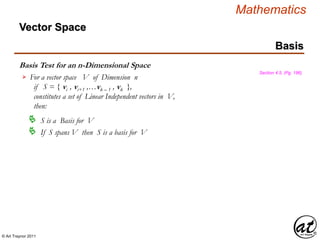
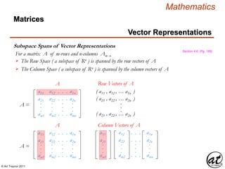
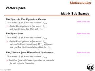
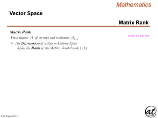
This document discusses mathematical expressions and equations. It defines key terms like expression, operand, operation, relation, polynomial, degree of a polynomial, quadratic polynomial, and equation. It also discusses the concept of a solution and solution set to an equation. Specifically, it defines a solution as a value substituted for a free variable that renders an equation true, and a solution set as the family or set of all possible solutions to an equation.


![© Art Traynor 2011
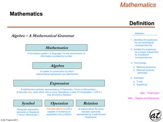
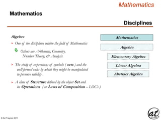
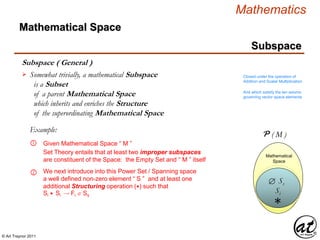
Mathematics
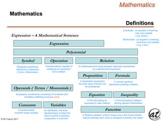
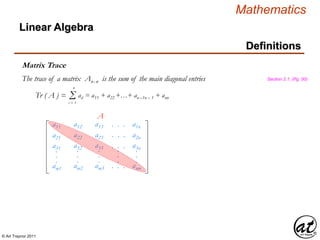
Definitions
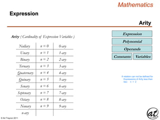
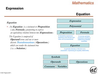
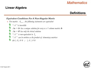
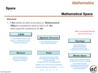
Expression
Symbol Operation Relation
Expression – A Mathematical Sentence
Proposition Formula
VariablesConstants
Operands ( Terms )
Equation
A formula stating an
equivalency class relation
Linear Equation
An equation in which each term is either
a constant or the product of a constant
and (a) variable[s] of the first degree
Mathematics
Polynomial](https://image.slidesharecdn.com/2d826fdb-8c8e-4ed6-a046-0eb4c5ad7212-160620064415/85/LinearAlgebra_160423_01-6-320.jpg)
![© Art Traynor 2011
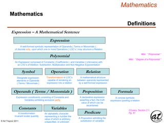
Mathematics
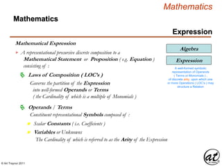
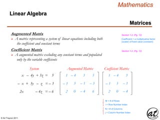
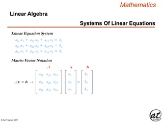
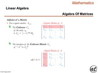
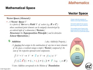
Linear Equation
Linear Equation
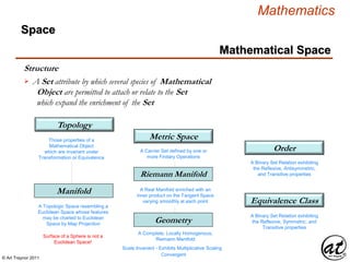
Equation
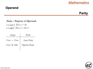
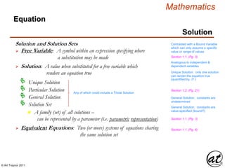
An Equation consisting of:
Operands that are either
Any Variables are restricted to the First Order n = 1
Linear Equation
An equation in which each term
is either a constant or the
product of a constant and (a)
variable[s] of the first order
Expression
Proposition
Equation
Formula
n Constant(s) or
n A product of Constant(s) and
one or more Variable(s)
The Linear character of the Equation derives from the
geometry of its graph which is a line in the R2 plane
As a Relation the Arity of a Linear Equation must be
at least two, or n ≥ 2 , or a Binomial or greater Polynomial
Polynomial](https://image.slidesharecdn.com/2d826fdb-8c8e-4ed6-a046-0eb4c5ad7212-160620064415/85/LinearAlgebra_160423_01-21-320.jpg)
![© Art Traynor 2011
Mathematics
Equation
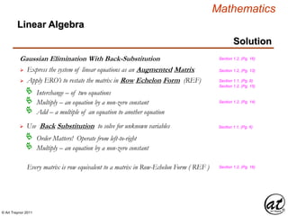
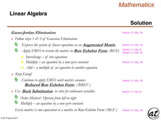
Linear Equation
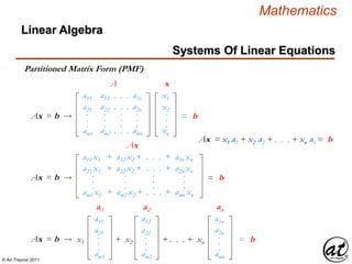
Linear Equation
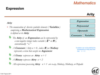
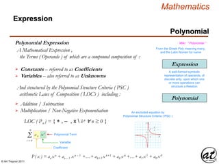
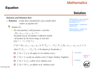
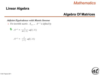
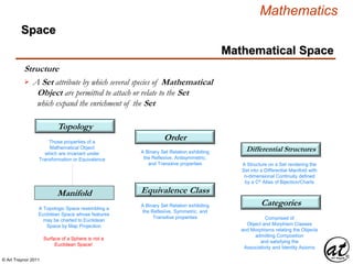
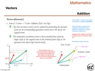
An equation in which each term is either a constant or the product
of a constant and (a) variable[s] of the first order
Term ai represents a Coefficient
b = Σi= 1
n
ai xi = ai xi + ai+1 xi+1…+ an – 1 xn – 1 + an xn
Equation of a Line in n-variables
A linear equation in “ n ” variables, xi + xi+1 …+ xn-1 + xn
has the form:
n Coefficients are distributed over a defined field
( e.g. N , Z , Q , R , C )
Term xi represents a Variable ( e.g. x, y, z )
n Term a1 is defined as the Leading Coefficient
n Term x1 is defined as the Leading Variable
Section 1.1, (Pg. 2)
Section 1.1, (Pg. 2)
Section 1.1, (Pg. 2)
Section 1.1, (Pg. 2)
Coefficient = a multiplicative factor
(scalar) of fixed value (constant)
Section 1.1, (Pg. 2)](https://image.slidesharecdn.com/2d826fdb-8c8e-4ed6-a046-0eb4c5ad7212-160620064415/85/LinearAlgebra_160423_01-22-320.jpg)
![© Art Traynor 2011
Mathematics
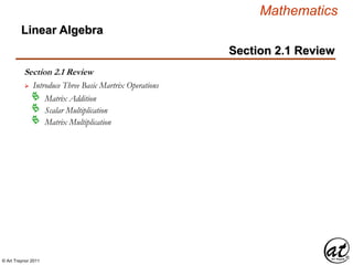
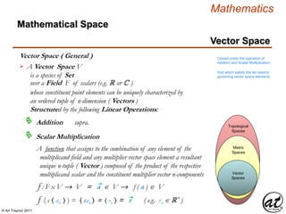
Linear Equation
Equation
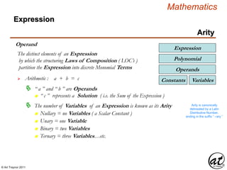
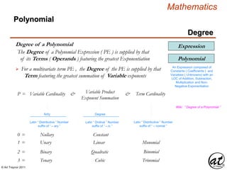
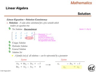
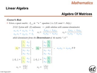
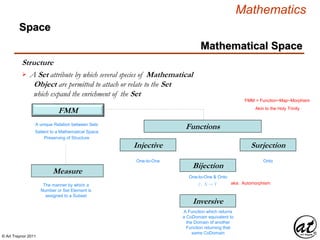
Standard Form ( Polynomial )
Ax + By = C
Ax1 + By1 = C
For the equation to describe a line ( no curvature )
the variable indices must equal one
ai xi + ai+1 xi+1 …+ an – 1 xn –1 + an xn = b
ai xi
1 + ai+1 x 1 …+ an – 1 x 1 + a1 x 1 = bi+1 n – 1 n n
ℝ
2
: a1 x + a2 y = b
ℝ
3
: a1 x + a2 y + a3 z = b
Blitzer, Section 3.2, (Pg. 226)
Section 1.1, (Pg. 2)
Test for Linearity
A Linear Equation can be expressed in Standard Form
As a species of Polynomial , a Linear Equation
can be expressed in Standard Form
Every Variable term must be of precise order n = 1
Linear Equation
An equation in which each term
is either a constant or the
product of a constant and (a)
variable[s] of the first order
Expression
Proposition
Equation
Formula
Polynomial](https://image.slidesharecdn.com/2d826fdb-8c8e-4ed6-a046-0eb4c5ad7212-160620064415/85/LinearAlgebra_160423_01-23-320.jpg)

![© Art Traynor 2011
Mathematics
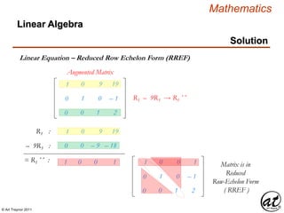
Matrix Representation
Linear Algebra
Matrix Representation Methods
Uppercase Letter Designation
Section 1.2, (Pg. 40)
A , B , C
Bracket-Enclosed Representative Element
[ aij ] , [ bij ] , [ cij ]
a11
a21
a31
am1
.
.
.
a12
a22
a32
am2
.
.
.
a13
a23
a33
am3
.
.
.
. . .
. . .
. . .
. . .
.
.
.
a1n
a2n
a3n
amn
.
.
.
Rectangular Array
Brackets denote a Matrix ( i.e. not a specific element/real number)](https://image.slidesharecdn.com/2d826fdb-8c8e-4ed6-a046-0eb4c5ad7212-160620064415/85/LinearAlgebra_160423_01-47-320.jpg)
![© Art Traynor 2011
Mathematics
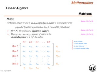
Matrix Equality
Linear Algebra
Matrix Equality Section 1.2, (Pg. 40)
A = [ aij ]
B = [ bij ]
are equal
when
Amxn = Bmxn
aij = bij
1 ≤ i ≤m
1 ≤ j ≤n
a1 a2 a3 . . . ana =
C1 C2 C3 . . . Cn
Row Matrix / Row Vector
A 1 x n (“ 1 by n ”) matrix is a single row
Column Matrix / Column Vector
b1
b2
b3
bm
.
.
.
C1
An m x 1 (“ m by 1 ”) matrix is a single column](https://image.slidesharecdn.com/2d826fdb-8c8e-4ed6-a046-0eb4c5ad7212-160620064415/85/LinearAlgebra_160423_01-48-320.jpg)
![© Art Traynor 2011
Mathematics
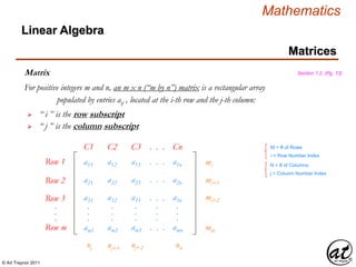
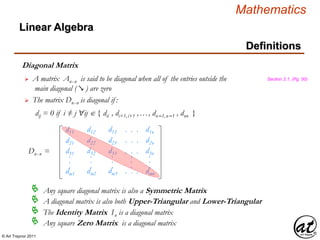
Matrix Operations
Linear Algebra
Matrix Summation Section 1.2, (Pg. 41)
A = [ aij ]
B = [ bij ]
is given
by
+ A + B = [ aij + bij ]
– 1
0
2
1
1
– 1
3
2
+ = ( – 1 + 1 ) =
( 0 + [ – 1] )
( 2 + 3 )
( 1 + 2 )
0
– 1
5
3
Scalar Multiplication
1
– 3
2
2
0
1
4
– 1
2
A = 3A =
3 ( 1 ) 3 ( 2 ) 3 ( 4 )
3 ( – 3 ) 3 ( 0 ) 3 ( – 1 )
3 ( 2 ) 3 ( 1 ) 3 ( 2 )
3
– 9
6
6
0
3
12
– 3
6
3A =](https://image.slidesharecdn.com/2d826fdb-8c8e-4ed6-a046-0eb4c5ad7212-160620064415/85/LinearAlgebra_160423_01-49-320.jpg)
![© Art Traynor 2011
Mathematics
Matrix Operations
Linear Algebra
Section 1.2, (Pg. 42)Matrix Multiplication
– 1
4
5
3
– 2
0
A =
A = [ aij ] Amx n
B = [ bij ] Bnx p
then AB = [ cij ] = Σk = 1
n
aik bkj = ai 1 b1 j + ai2 b2j +…+ ain –1 bn-1j + ain bnj
The entries of Row “ Aik” ( the i-th row ) are multiplied by the entries of “ Bkj” ( the j-th column )
and sequentially summed through Row “ Ain” and Column “ Bnj” to form the entry at [ cij ]
– 3
– 4
2
1
B =
c11 c12
C = c21 c22
c31 c32
a11b11 + a12b21 a11b12 + a12b22
= a21b11 + a22b21 a21b12 + a22b22
a31b11 + a32b21 a31b12 + a32b22
Product Summation Operand Count
For Each Element of AB (single entry)
Product Summation (Column-Row) Index
For the product of two matrices to be defined, the column count of the multiplicand matrix
must equal the row count of the multiplier matrix ( i.e. Ac = Br )
ABmx p](https://image.slidesharecdn.com/2d826fdb-8c8e-4ed6-a046-0eb4c5ad7212-160620064415/85/LinearAlgebra_160423_01-50-320.jpg)
![© Art Traynor 2011
Mathematics
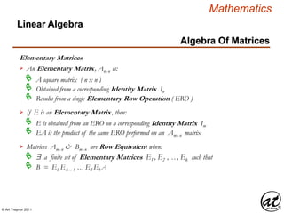
Algebra Of Matrices
Linear Algebra
Proofs
Let A = [ aij ], B = [ bij ]
Introduce/Define/Declare The Constituents to be Proven
This statement declares A & B to be Matrices
Specifies the row & column count index variables](https://image.slidesharecdn.com/2d826fdb-8c8e-4ed6-a046-0eb4c5ad7212-160620064415/85/LinearAlgebra_160423_01-55-320.jpg)
![© Art Traynor 2011
Mathematics
Algebra Of Matrices
Linear Algebra
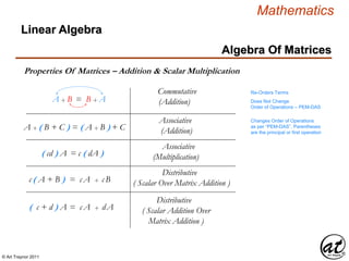
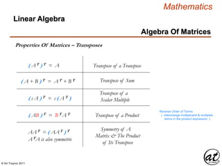
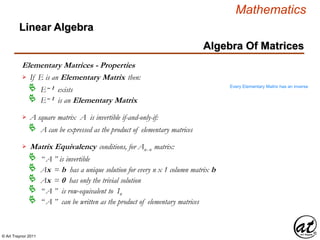
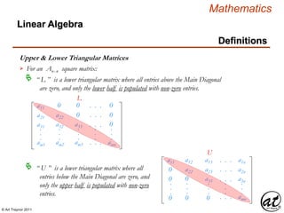
Properties Of Matrices – Proofs
A( BC ) = ( AB ) C
Order of Terms is preserved
Affects Order of Operations
Sequence – PEM-DAS
Associative
(Multiplication)
Σk = 1
n
T = [ tij ] = ( aik bkj )ckjΣk = 1
n
Σi = 1
n
( yj )Σj = 1
n
( xi )
Σi = 1
n
( xi ) ( y1 + y2 +…+ yn –1 + yn )
( x1 + x2 +…+ xn –1 + xn ) y1 + ( x1 + x2 +…+ xn –1 + xn ) y2 +…
( x1 + x2 +…+ xn –1 + xn ) yn –1 + ( x1 + x2 +…+ xn –1 + xn ) yn
x1 y1 + x2 y1 +…+ xn –1 y1 + xn y1 + x1 y2 + x2 y2 +…+ xn –1 y2 + xn y2 +…
x1 yn –1 + x2 yn –1 +…+ xn –1 yn –1 + xn yn –1 + x1 yn + x2 yn +…+ xn –1 yn + xn yn](https://image.slidesharecdn.com/2d826fdb-8c8e-4ed6-a046-0eb4c5ad7212-160620064415/85/LinearAlgebra_160423_01-58-320.jpg)
![© Art Traynor 2011
Mathematics
Algebra Of Matrices
Linear Algebra
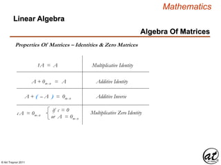
Properties Of Matrices – Proofs
A( BC ) = ( AB ) C
Order of Terms is preserved
Affects Order of Operations
Sequence – PEM-DAS
Associative
(Multiplication)
Σk = 1
n
T = [ tij ] = ( aik bkj )ckjΣk = 1
n
Σi = 1
n
( yj )Σj = 1
n
( xi )
Σi = 1
n
( xi ) ( y1 + y2 +…+ yn –1 + yn )
( x1 + x2 +…+ xn –1 + xn ) y1 + ( x1 + x2 +…+ xn –1 + xn ) y2 +…
( x1 + x2 +…+ xn –1 + xn ) yn –1 + ( x1 + x2 +…+ xn –1 + xn ) yn
x1 y1 + x2 y1 +…+ xn –1 y1 + xn y1 + x1 y2 + x2 y2 +…+ xn –1 y2 + xn y2 +…
x1 yn –1 + x2 yn –1 +…+ xn –1 yn –1 + xn yn –1 + x1 yn + x2 yn +…+ xn –1 yn + xn yn
Σi = 1
n
Σj = 1
n
xi yj](https://image.slidesharecdn.com/2d826fdb-8c8e-4ed6-a046-0eb4c5ad7212-160620064415/85/LinearAlgebra_160423_01-59-320.jpg)
![© Art Traynor 2011
Mathematics
Algebra Of Matrices
Linear Algebra
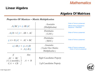
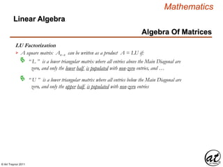
Properties Of Matrices – Proofs
A = [ aij ] Amx n
B = [ bij ] Bnx p
then AB = [ cij ] = Σk = 1
n
aik bkj = ai 1 b1 j + ai2 b2j +…+ ain –1 bn-1j + ain bnj
Product Summation Operand Count
Product Summation (Column-Row) Index
ABmx p
The entries of Row “ Aik” ( the i-th row ) are multiplied by the entries of “ Bkj” ( the j-th column )
and sequentially summed through Row “ Ain” and Column “ Bnj” to form the entry at [ cij ]
ai,1 b1, j + ai,1 b1, j +1 ai,1 b1,n – 1 + ai,1 b1,n
ai+1,2 b2, j + ai+1,2 b2, j +1 ai+1,2 b2, n – 1 + ai+1,2 b2, n
.
.
.
.
.
.
.
.
.
+ . . .+
+ . . .+
.
.
.
.
.
.
an – 1,n – 1bn – 1, j + an – 1,n – 1bn – 1, j +1 an – 1,n – 1bn – 1, n – 1 + an – 1,n – 1bn
an,nbn, j + an,n bn, j +1 an,n bn,n – 1 + an,n bn,n
+ . . .+
+ . . .+
Section 1.2, (Pg. 42)
For Each Element of AB (single entry)](https://image.slidesharecdn.com/2d826fdb-8c8e-4ed6-a046-0eb4c5ad7212-160620064415/85/LinearAlgebra_160423_01-60-320.jpg)
![© Art Traynor 2011
Mathematics
Algebra Of Matrices
Linear Algebra
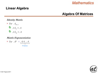
Transpose Matrix
a11
a21
am1
.
.
.
a12
a22
am2
.
.
.
. . .
. . .
. . .
.
.
.
a1n
a2n
amn
.
.
.
A =
a11
a12
a1n
.
.
.
a21
a22
a2n
.
.
.
. . .
. . .
. . .
.
.
.
am1
am2
amn
.
.
.
AT =
1
2
0
2
1
0
0
0
1
C =
1
2
0
2
1
0
0
0
1
CT =
Symmetric Matrix: C = CT
If C = [ cij ] is a symmetric matrix, cij = cji for i ≠ j
C = [ cij ] is a symmetric matrix, Cmx n = CT
nx p for m = n = p](https://image.slidesharecdn.com/2d826fdb-8c8e-4ed6-a046-0eb4c5ad7212-160620064415/85/LinearAlgebra_160423_01-62-320.jpg)
![© Art Traynor 2011
Mathematics
Algebra Of Matrices
Linear Algebra
1
2
0
2
1
0
0
0
1
C =
1
2
0
2
1
0
0
0
1
CT =
If C = [ cij ] is a symmetric matrix, cij = cji , "i,j | i ≠ j
C = [ cij ] is a symmetric matrix, Cmx n = CT
nx p , "m,n, p | m = n = p
Symmetric Matrix
A Symmetric Matrix is a
Square Matrix that is
equal to it Transpose ( e.g. Cmx n = CT
mx n , "m,n | m = n)
](https://image.slidesharecdn.com/2d826fdb-8c8e-4ed6-a046-0eb4c5ad7212-160620064415/85/LinearAlgebra_160423_01-63-320.jpg)
![© Art Traynor 2011
Mathematics
Algebra Of Matrices
Linear Algebra
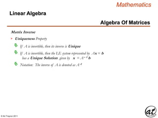
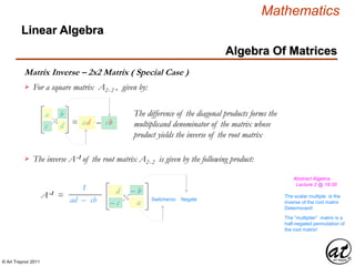
Matrix Inverse
A matrix Anx n is Invertible or Non-Singular when
$ matrix Bnx n | AB = BA = In
In : Identity Matrix of Order n
Bnx n : The Multiplicative Inverse of A
A matrix that does not have an inverse is Non-Invertible or Singular
Non-square matrices do not have inverses
n For matrix products Amx n Bnx p where m ≠ n ≠ p,
AB ≠ BA as [ aij ≠ bij ] ??
](https://image.slidesharecdn.com/2d826fdb-8c8e-4ed6-a046-0eb4c5ad7212-160620064415/85/LinearAlgebra_160423_01-65-320.jpg)
![© Art Traynor 2011
Mathematics
Algebra Of Matrices
Linear Algebra
Matrix Inverse
There are two methods for determining an inverse matrix A-1
of A ( if an inverse exists):
Solve Ax = In for X
Adjoin the Identity Matrix In (on RHS ) to A forming the doubly-
augmented matrix [ A In ] and perform EROs concluding in RREF to
produce an [ In A-1 ] solution
A test for determining whether an inverse matrix A-1 of A exists:
Demonstrate that either/or AB = In = BA
Section 2.3 (Pg. 64)](https://image.slidesharecdn.com/2d826fdb-8c8e-4ed6-a046-0eb4c5ad7212-160620064415/85/LinearAlgebra_160423_01-66-320.jpg)
![© Art Traynor 2011
Mathematics
Algebra Of Matrices
Linear Algebra
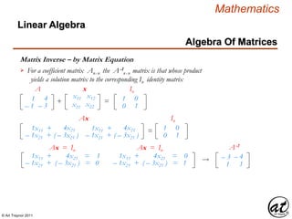
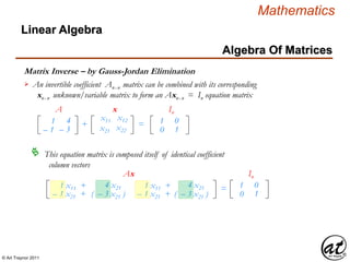
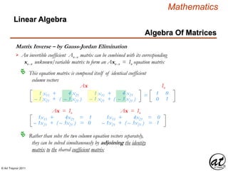
Matrix Inverse – by Gauss-Jordan Elimination ( GJE )
An invertible coefficient Anx n matrix can be combined with its corresponding
xnx n unknown/variable matrix to form an Axnx n = In equation matrix
This equation matrix is composed itself of identical coefficient
column vectors
1 x11 + 4 x21 = 1
– 1 x21 + ( – 3 x21 ) = 0
1 x11 + 4 x21 = 0
– 1 x21 + ( – 3 x21 ) = 1
Ax = In Ax = In
Rather than solve the two column equation vectors separately,
they can be solved simultaneously by adjoining the identity
matrix to the shared coefficient matrix…
1
– 1
4
– 3
A
1
0
0
1
In
…then execute ERO’s to effect a GJ-Elimination of the
“ doubly augmented ” [ A I ] matrix the conclusion of
which will yield an [ I A-1 ] inverse matrix](https://image.slidesharecdn.com/2d826fdb-8c8e-4ed6-a046-0eb4c5ad7212-160620064415/85/LinearAlgebra_160423_01-71-320.jpg)
![© Art Traynor 2011
Mathematics
Algebra Of Matrices
Linear Algebra
Matrix Inverse – by Gauss-Jordan Elimination
An invertible coefficient Anx n matrix can be combined with its corresponding
xnx n unknown/variable matrix to form an Axnx n = In equation matrix
This equation matrix is composed itself of identical coefficient
column vectors
1 x11 + 4 x21 = 1
– 1 x21 + ( – 3 x21 ) = 0
1 x11 + 4 x21 = 0
– 1 x21 + ( – 3 x21 ) = 1
Ax = In Ax = In
The adjoined, “ doubly-augmented ” coefficient matrix , by means of ERO’s , is reduced by
GJ-Elimination to produce the [ I A-1 ] inverse matrix
1
– 1
4
– 3
A
1
0
0
1
In
– 3
1
– 4
1
A-1
1
0
0
1
In
Which is confirmed by verifying either of the following
n AA-1 = I
n AA-1 = A-1 A](https://image.slidesharecdn.com/2d826fdb-8c8e-4ed6-a046-0eb4c5ad7212-160620064415/85/LinearAlgebra_160423_01-72-320.jpg)
![© Art Traynor 2011
Mathematics
Linear Algebra
Definitions
EROs & Determinants (Properties)
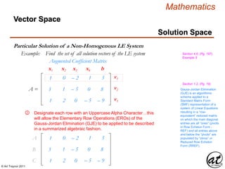
Permutation:
[ A ] Pij [ B ]
det ( B ) = – det ( A )
|B | = – | A |
Multiplication by a Scalar:
[ A ] cRi [ B ]
det ( B ) = c det ( A )
|B | = c | A |
Addition to a Row Multiplied by a Scalar:
[ A ] Ri + cRj [ B ]
det ( B ) = det ( A )
|B | = | A |
There are three “effects” to a resultant
matrix which are unique to each of the
three EROs
Permutation
Scalar Multiplication
Row Addition](https://image.slidesharecdn.com/2d826fdb-8c8e-4ed6-a046-0eb4c5ad7212-160620064415/85/LinearAlgebra_160423_01-89-320.jpg)


![© Art Traynor 2011
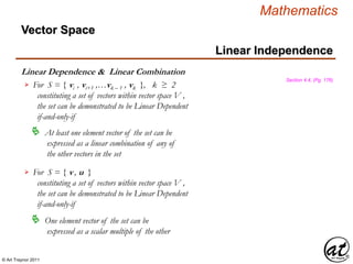
Mathematics
Definition
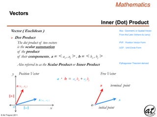
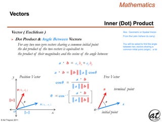
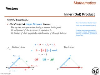
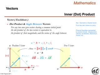
Vectors
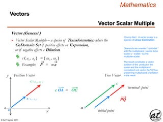
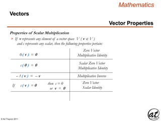
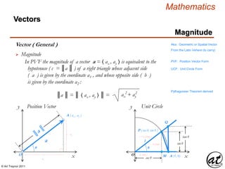
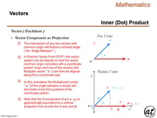
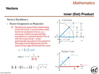
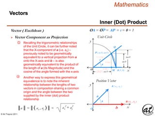
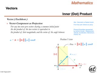
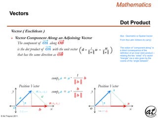
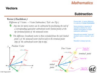
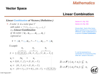
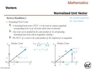
Vector ( Euclidean )
A geometric object (directed line segment)
describing a physical quantity and characterized by
Direction: depending on the coordinate system used to describe it; and
Magnitude: a scalar quantity (i.e. the “length” of the vector)
Aka: Geometric or Spatial Vector
originating at an initial point [ an ordered pair : ( 0, 0 ) ]
and concluding at a terminal point [ an ordered pair : ( a1 , a2 ) ]
Other mathematical objects
describing physical quantities and
coordinate system transforms
include: Pseudovectors and
Tensors
Not to be confused with elements of Vector Space (as in Linear Algebra)
Fixed-size, ordered collections
Aka: Inner Product Space
Also distinguished from statistical concept of a Random Vector
From the Latin Vehere (to carry)
or from Vectus…to carry some-
thing from the origin to the point
constituting the components of the vector 〈 a1 , a2 〉](https://image.slidesharecdn.com/2d826fdb-8c8e-4ed6-a046-0eb4c5ad7212-160620064415/85/LinearAlgebra_160423_01-142-320.jpg)


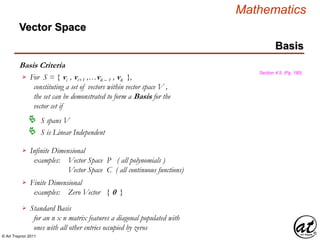
![© Art Traynor 2011
Mathematics
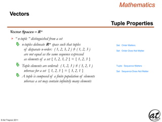
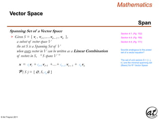
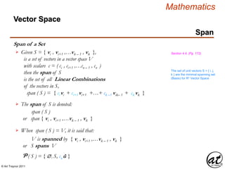
Vector Spaces
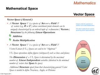
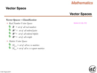
Vector Spaces – Classification
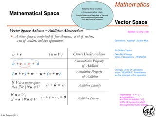
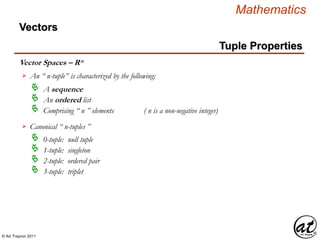
Polynomial Vector Spaces
P = set of all polynomials
Pn = set of all polynomials of degree ≤ n
Continuous Functions ( Calculus ) Vector Spaces
C ( – ∞ , ∞) = set of all continuous functions
defined on the real number line
C [ a, b ] = set of all continuous functions
defined on a closed interval [ a, b ]
Section 4.2, (Pg. 157)
Vector Space](https://image.slidesharecdn.com/2d826fdb-8c8e-4ed6-a046-0eb4c5ad7212-160620064415/85/LinearAlgebra_160423_01-150-320.jpg)
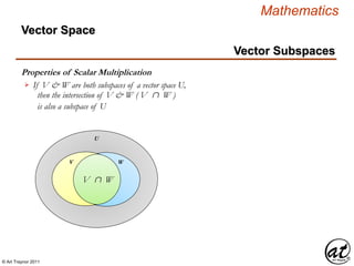
![© Art Traynor 2011
Mathematics
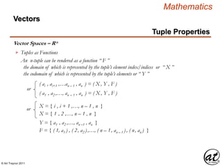
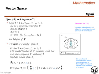
Vector Subspaces
W 1
Polynomial
functions
W 5
Functions
W 2
Differentiable
functions
W 3
Continuous
functions
W 4
Integrable
functions
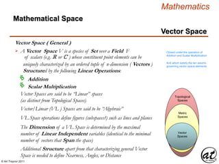
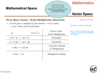
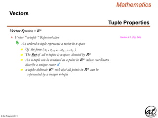
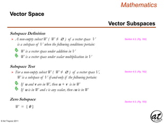
W5 = Vector Space " f Defined on [ 0, 1 ]
W4 = Set " f Integrable on [ 0, 1 ]
W3 = Set " f Continuous on [ 0, 1 ]
W2 = Set " f Differentiable on [ 0, 1 ]
W2 = Set " Polynomials
Defined on [ 0, 1 ]
W1 W2 W3 W4 W5
W 1 – Every Polynomial function is Differentiable W1 W2
W 2 – Every Differentiable function is Continuous W2 W3
W 3 – Every Continuous function is Integrable W3 W4
W 4 – Every Integrable function
is a Function W4 W5
Function Space Section 4.3, (Pg. 164)
Vector Space](https://image.slidesharecdn.com/2d826fdb-8c8e-4ed6-a046-0eb4c5ad7212-160620064415/85/LinearAlgebra_160423_01-152-320.jpg)

![© Art Traynor 2011
Mathematics
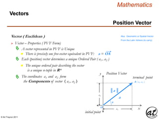
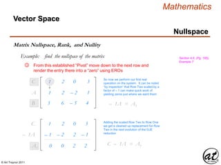
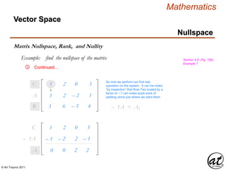
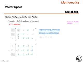
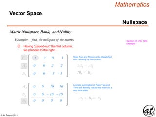
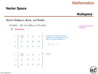
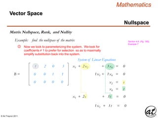
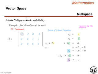
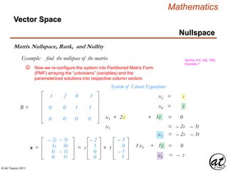
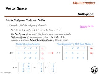
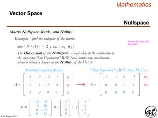
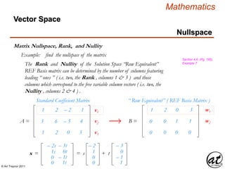
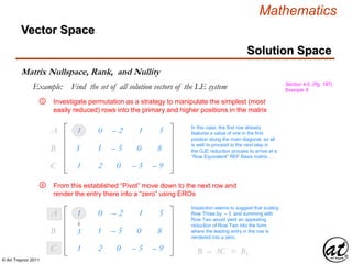
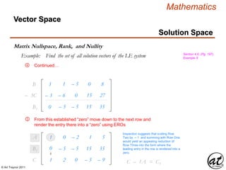
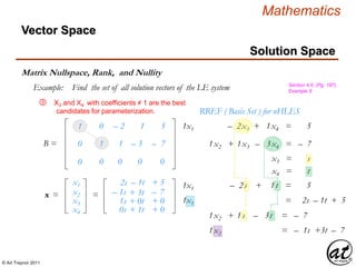
Matrix Nullspace and Nullity
Nullspace
Section 4.6, (Pg. 194)
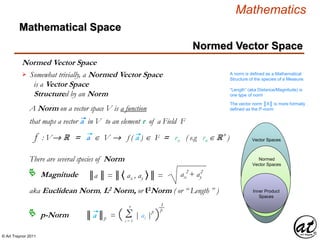
The solution set for the system forms a subspace of Rn designated as
the Nullspace of A and denoted as N ( A )
Vector Space
For a homogenous linear system Ax = 0 where A is an matrix of m-rows
and n-columns Amx n , x = [ xi , xi+1 ,…xn – 1 , xn ] T is a column
vector of unknowns 0 = [ 0 , 0 , … 0 , 0 ] T is the zero vector in Rm
N ( A ) = { x Rn | Ax = 0 }
The Dimension of the Nullspace of A is designated as its Nullity
dim ( N ( A ) )](https://image.slidesharecdn.com/2d826fdb-8c8e-4ed6-a046-0eb4c5ad7212-160620064415/85/LinearAlgebra_160423_01-175-320.jpg)

![© Art Traynor 2011
Mathematics
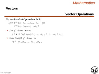
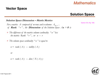
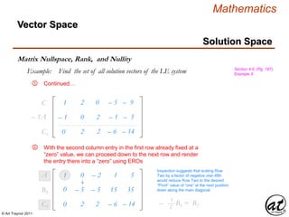
Solution Space Consistency
Solution Space
Section 4.6, (Pg. 198)
Vector Space
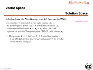
For a matrix A composed of m-rows and n-columns Amx n ,
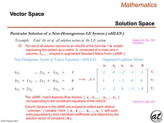
of which Ax = b defines a particular solution xp to the nHLES
The nHLES is consistent if-and-only-if
The solution vector b is among the Column Space of A
The solution vector b = [ bi , bi+1 ,…bn – 1 , bn ] T
represents a Linear Combination of the columns of A
The solution vector b is among those populating the Subspace Rm
Spanned by the columns of A
There is an additional
implication that the respective
Ranks of the nHLES
coefficient and augmented
matrices are equivalent
Section 4.6, (Pg. 198)
I think what is meant by this
is that if b is adjoined to A
then reduced by GJE to an RREF
matrix B, so long as the column
representing b remains, the system is thus
demonstrated consistent](https://image.slidesharecdn.com/2d826fdb-8c8e-4ed6-a046-0eb4c5ad7212-160620064415/85/LinearAlgebra_160423_01-203-320.jpg)
![© Art Traynor 2011
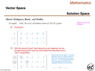
Mathematics
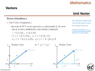
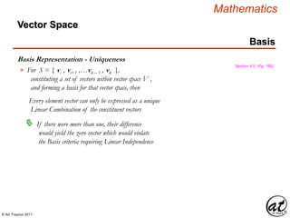
Coordinate Representation Relative to a Basis
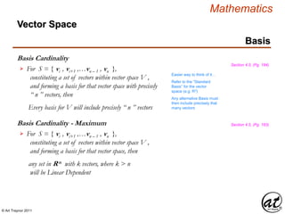
Basis
Section 4.7, (Pg. 202)
Vector Space
For an Ordered Basis set B = { vi , vi+1 ,…vn – 1 , vn },
within Vector Space V , there exists a vector x in V
that can be expressed as a Linear Combination, or sum of
scalar multiples of the constituent vectors of x such that:
xn = ci vi + ci+1 vi+1 +…+ cn –1 vn – 1 + cn vn
The coordinate matrix, or coordinate vector, of x relative to B is the
column matrix in Rn whose components are the coordinates of x
the scalars of which ci = [ ci , ci+1 ,…cn – 1 , cn ] are otherwise
referred to as the coordinates of x relative to the Basis B
c1
c2
cn
.
.
.
[ xn ]Bn
=
Chump Alert: Coordinate
matrix representation relative
to a Basis ( standard or
otherwise) is directly
analogous to Normalized ( ? )
Unit Vector representation](https://image.slidesharecdn.com/2d826fdb-8c8e-4ed6-a046-0eb4c5ad7212-160620064415/85/LinearAlgebra_160423_01-205-320.jpg)
![© Art Traynor 2011
Mathematics
y´
Vector Space
Basis
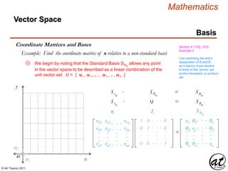
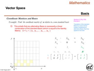
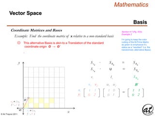
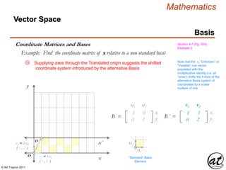
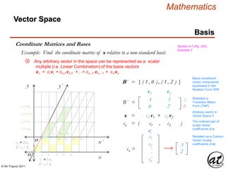
Coordinate Matrices and Bases Section 4.7 (Pg. 203),
Example 2
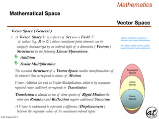
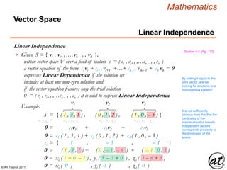
Example: Find the coordinate matrix of x relative to a non-standard basis
the ordered pair collection of vector scalar coefficients of the arbitrary
vector x is explicitly corresponded with the Basis vectors the
products of which form a resultant Linear Combination.
x
y
x´
O
O ´
1B 2B 3B 4B 5B
1B ⇌ ½B´
1B´ 2B´ 3B´
2B ⇌ 1B´
3B ⇌ 1½ B´
4B ⇌ 2B´
v2 = 2 u2
( 1 , 2 )
v1 = 1 u1
( 1 , 0 )
xn = c1 v1 + c2 v2
cn = ( c1 , c2 )
A scalar coefficient of
“one” is implicit
c1
c2
cn
.
.
.
ci
311
221
The ordered pair of
scalar vector
coefficients of x
Restated as a Column
Vector (scalar
coefficients of x)
B´ = { v1 , v2 }
The set of Basis
vectors in SNF
Juxtaposed as below,
it is clear that x is a
linear combination of
the Basis Vectors
B´ = { 1 v1 , 1 v2 }
ci ≠ 1 implies that the
arbitrary vector is a
Linear Combination of
the Basis Vector set
cn = [ x ]B´ =
An illuminating change of notation is here introduced [ x ]B´ whereby
1B´ 2B´ 3B´ 4B´ 5B´
5a](https://image.slidesharecdn.com/2d826fdb-8c8e-4ed6-a046-0eb4c5ad7212-160620064415/85/LinearAlgebra_160423_01-215-320.jpg)
![© Art Traynor 2011
Mathematics
y´
Vector Space
Basis
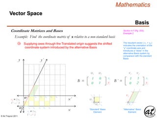
Coordinate Matrices and Bases Section 4.7 (Pg. 203),
Example 2
Example: Find the coordinate matrix of x relative to a non-standard basis
x
y
x´
O
O ´
1B 2B 3B 4B 5B
1B ⇌ ½B´
1B´ 2B´ 3B´
2B ⇌ 1B´
3B ⇌ 1½ B´
4B ⇌ 2B´
v2 = 2 u2
( 1 , 2 )
v1 = 1 u1
( 1 , 0 )
c1
c2
cn
.
.
.
ci
311
221
Stated as a Column
Vector (scalar
coefficients of x)
Juxtaposed as below,
it is clear that x is a
linear combination of
the Basis Vectors
cn = [ x ]B´ =
The novel notation for the set (ordered pair, or column vector form)
of vector scalar coefficients ci directs our attention to the specific
Basis by which the resulting coordinates are generated.
e.g.: x is expressed relative to Basis B
“ Relative to ”
“ Defined by ”
“ Within ”
xn = c1 v1 + c2 v2
cn = ( c1 , c2 )
B´ = { v1 , v2 }
B´ = { 1 v1 , 1 v2 }1B´ 2B´ 3B´ 4B´ 5B´
5b](https://image.slidesharecdn.com/2d826fdb-8c8e-4ed6-a046-0eb4c5ad7212-160620064415/85/LinearAlgebra_160423_01-216-320.jpg)
![© Art Traynor 2011
Mathematics
y´
Vector Space
Basis
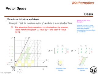
Coordinate Matrices and Bases Section 4.7 (Pg. 203),
Example 2
Example: Find the coordinate matrix of x relative to a non-standard basis
①
x
y
x´
O
O ´
1B 2B 3B 4B 5B
1B ⇌ ½B´
1B´ 2B´ 3B´
2B ⇌ 1B´
3B ⇌ 1½ B´
4B ⇌ 2B´
v2 = 2 u2
( 1 , 2 )
v1 = 1 u1
( 1 , 0 )
c1
c2
cn
.
.
.
ci
311
221
Stated as a Column
Vector (scalar
coefficients of x)
Juxtaposed as below,
it is clear that x is a
linear combination of
the Basis Vectors
cn = [ x ]B´ =
Vector x therefore can be graphically represented by a Position
Vector demarcated in the B-Prime coordinate system [ i.e. three
increments of “ x ” from the alternative Basis ( aB ) origin and two
increments of “ y ” from the aB origin ].
“ Relative to ”
“ Defined by ”
“ Within ”
111 012
021 122
B
u1 u2
u2
u1
v2
v1
111 112
021 222
B ´
v1 v2
xi
yj
“Standard” Basis
Element
“Alternative” Basis
Element
1B
1B
1B´
2B ⇌ 1B´
xB = ( 3 , 2 )
1B´ 2B´ 3B´ 4B´ 5B´](https://image.slidesharecdn.com/2d826fdb-8c8e-4ed6-a046-0eb4c5ad7212-160620064415/85/LinearAlgebra_160423_01-217-320.jpg)
![© Art Traynor 2011
Mathematics
y´
Vector Space
Basis
Coordinate Matrices and Bases Section 4.7 (Pg. 203),
Example 2Example: Find the coordinate matrix of x relative to a non-standard basis
①
x
y
x´
O
O ´
1B 2B 3B 4B 5B
1B ⇌ ½B´
1B´ 2B´ 3B´
2B ⇌ 1B´
3B ⇌ 1½ B´
4B ⇌ 2B´
v2 = 2 u2
( 1 , 2 )
v1 = 1 u1
( 1 , 0 )
To restate the scalar set of the arbitrary vector
coefficients in terms of the standard basis ( sB ),
the aB vector components need simply be scaled
by the vector equation for x to yield the scalar
solution set in terms of the sB
xB = ( 3 , 2 )
xn = c1 v1 + c2 v2
B´ = { ( 1 , 0 ) , ( 1 , 2 ) }
B´ = { v1 , v2 }
xn = c1 ( 1 , 0 ) + c2 ( 1 , 2 )
cn = [ x ]B
= ( c1 , c2 )
cn = [ x ]B
= ( 3 , 2 )
xn = 3( 1 , 0 ) + 2 ( 1 , 2 )
x = ( 3·1 + 2·1 ) , ( 3·0 + 2·2 )
x = ( 3 + 2 ) , ( 0 + 4 )
x = ( 5 ) , ( 4 )
xn = 3 ( v1 ) + 2 ( v2 )
1B´ 2B´ 3B´ 4B´
5B´](https://image.slidesharecdn.com/2d826fdb-8c8e-4ed6-a046-0eb4c5ad7212-160620064415/85/LinearAlgebra_160423_01-218-320.jpg)
![© Art Traynor 2011
Mathematics
Vector Space
Basis
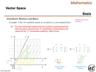
Coordinate Matrices and Bases Section 4.7 (Pg. 203),
Example 2Example: Find the coordinate matrix of x relative to a non-standard basis
① Note finally that, as B ′ ( B-Prime ) is the Identity
Matrix ( IM ), the B matrix is equivalent to the
Transition Matrix (from non-standard to standard
Basis) conventionally noted as P – 1
Section 4.7 (Pg. 208)
[ B′ In ]
Adjoin
[ In P – 1 ]
RREF
GJE
( EROs )
P – 1 = ( B′ ) – 1
′
Change of Basis
Non-Standard Standard
111 112
021 222
v1 v2
xi
yj
P – 1 = ( B′ ) = ′](https://image.slidesharecdn.com/2d826fdb-8c8e-4ed6-a046-0eb4c5ad7212-160620064415/85/LinearAlgebra_160423_01-219-320.jpg)
![© Art Traynor 2011
Mathematics
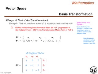
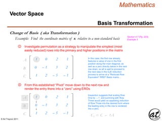
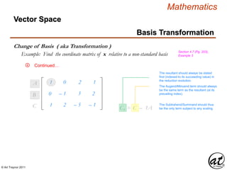
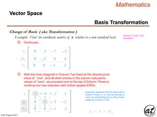
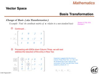
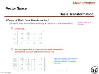
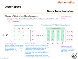
Change of Basis ( aka Transformation )
Basis Transformation
Vector Space
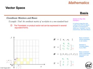
Section 4.7 (Pg. 203),
Example 3
Example: Find the coordinate matrix of x relative to a non-standard basis
With this restatement, we next introduce the arbitrary vector
coordinates ( to which we are tasked to find the coordinate matrix
corresponding to the aB ) rendering it into a column vector form.
①
B´ = { u1 , u2 , u3 }
B´ = { ( 1 , 0, 1 ) , ( 0 , – 1, 2 ) , ( 2 , 3, – 5 ) }
1
0
1
0
– 1
2
– 2
– 3
– 5
aB Coefficient Matrix
B´ =
c1
c2
c3
u1 u2 u3
These given arbitrary
vector coordinates are
presumably introduced
relative to the Standard
Basis?
xn = ( 1 , 2 , – 1 )
c1
c2
cn
.
.
.
ci
cn = [ x ]B´ =
1
2
c1
c2
c3
xi
– 1“ Relative to ”
“ Defined by ”
“ Within ”
Keep in mind that the ‘given’ arbitrary vector is stated relative to the
standard Basis and thus represents a solution set by which the set of
scalar multiples applicable to the alternative Basis will be derived.
Alternative Basis
constituent vectors
expressed in Set
Notation Form SNF](https://image.slidesharecdn.com/2d826fdb-8c8e-4ed6-a046-0eb4c5ad7212-160620064415/85/LinearAlgebra_160423_01-221-320.jpg)
![© Art Traynor 2011
Mathematics
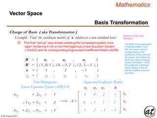
Change of Basis ( aka Transformation )
Basis Transformation
Vector Space
Section 4.7 (Pg. 203),
Example 3Example: Find the coordinate matrix of x relative to a non-standard basis
We next introduce a column vector of scalars the solution to which
will represent the coordinate matrix of the arbitrary vector with
respect to the alternative Basis ( aB )
①
B´ = { u1 , u2 , u3 }
B´ = { ( 1 , 0, 1 ) , ( 0 , – 1, 2 ) , ( 2 , 3, – 5 ) }
1
0
1
0
– 1
2
– 2
– 3
– 5
aB Coefficient Matrix
u1 u2 u3
Alternative Basis
constituent vectors
expressed in Set
Notation Form SNF
These given arbitrary
vector coordinates are
presumably introduced
relative to the Standard
Basis?
1
2
– 1
c1
c2
c3
xi
xn = ( 1 , 2 , – 1 )
Keep in mind that the ‘given’
arbitrary vector is stated relative
to the standard Basis and thus
represents a solution set by
which the set of scalar multiples
associated with the alternative
Basis will be determined
c1
c2
ci
– c3
=
cn = [ x ]B
= ( c1 , c2 , c3 )](https://image.slidesharecdn.com/2d826fdb-8c8e-4ed6-a046-0eb4c5ad7212-160620064415/85/LinearAlgebra_160423_01-222-320.jpg)
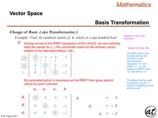
![© Art Traynor 2011
Mathematics
Vector Space
Basis Transformation
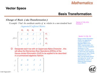
Change of Basis ( aka Transformation )
Section 4.7 (Pg. 203),
Example 3Example: Find the coordinate matrix of x relative to a non-standard basis
No parameterization is necessary as the RREF form gives explicit
values for each unknown
1 0 – 0 5
0 – 1 – 0 – 8
– 0 0 – 1 – 2
1d1 + 0x2 + 2c3 = 5s
3x1 – 1d2 + 3c3 = – 8s
1c1 + 2c2 – 5d3 = – 2s
u1 u2 u3 b
10
5
– 2
d1
d2
d3
xi
– 1
d1
d2
dn
.
.
.
di
dn = [ x ]B´ =
“ Relative to ”
“ Defined by ”
“ Within ”
5
– 2
d1
d2
d3
xi
– 1
d1
d2
d3
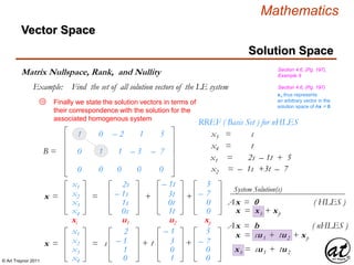
x = d1u1 + d2u2 + d3u3 + xp
System Solution(s)
x = xh + xp
xh = d1u1 + d2u2 + d3u3
Ax = b
Ax = 0 ( HLES )
( nHLES )
RREF ( Basis Set ) for nHLES](https://image.slidesharecdn.com/2d826fdb-8c8e-4ed6-a046-0eb4c5ad7212-160620064415/85/LinearAlgebra_160423_01-233-320.jpg)
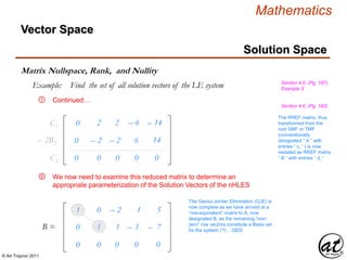
![© Art Traynor 2011
Mathematics
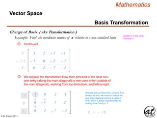
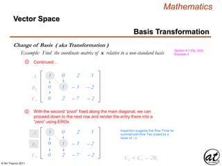
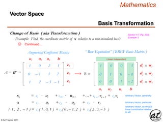
Change of Basis ( aka Transformation )
Basis Transformation
Vector Space
Section 4.7 (Pg. 203),
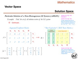
Example 3
Example: Find the coordinate matrix of x relative to a non-standard basis
Continued…13
d1
d2
dn
.
.
.
di
dn = [ x ]B´ =
“ Relative to ”
“ Defined by ”
“ Within ”
5
– 2
d1
d2
d3
xi
– 1
xn = ci · ui + ci+1 · ui+1 +…+ cn –1 vn – 1 + cn vn
Arbitrary Vector, generally
xnn = c1 · u1 + c2 · u2 + c3 · v3
Arbitrary Vector, particular
xn = 51 ( 1 , 0, 1 ) + ( – 82 ) ( 0 , – 1, 2 ) + ( – 22 )( 2 , 3, – 5 )
Arbitrary Vector, as nHLES
linear combination relative
to aB](https://image.slidesharecdn.com/2d826fdb-8c8e-4ed6-a046-0eb4c5ad7212-160620064415/85/LinearAlgebra_160423_01-236-320.jpg)
![© Art Traynor 2011
Mathematics
Change of Basis ( via Transition Matrix)
Basis Transformation
Vector Space
Section 4.7 (Pg. 204)
For an arbitrary vector x in vector space V described by coordinates relative to
a Standard Basis B , an ancillary description – in coordinate terms relative
to an Alternate Basis B′ ( B-Prime ) – can be determined by operation
of a Transition Matrix P ( the entries of which are populated by the
components of x ) .
The matrix product of P and a column vector [ x ]B′ of scalars
ci = [ ci , ci+1 ,…cn – 1 , cn ] which forms the coordinate matrix
of x relative to the alternate basis B′ ( B-Prime ) yield the
column vector [ x ]B′ , the “ root ” basis.
The “ Change of Basis ” is thus the solution to the unknown column
vector [ x ]B′ of scalars ci = [ ci , ci+1 ,…cn – 1 , cn ] .
](https://image.slidesharecdn.com/2d826fdb-8c8e-4ed6-a046-0eb4c5ad7212-160620064415/85/LinearAlgebra_160423_01-237-320.jpg)
![© Art Traynor 2011
Mathematics
Change of Basis ( via Transition Matrix)
Basis Transformation
Vector Space
Section 4.7 (Pg. 204)
The matrix product of P and a column vector [ x ]B′ of scalars
ci = [ ci , ci+1 ,…cn – 1 , cn ] which forms the coordinate matrix
of x relative to the alternate basis B′ ( B-Prime ) yield the
column vector [ x ]B′ .
P = B´ = { u1 , u2 , u3 }
P = B´ = { ( 1 , 0, 1 ) , ( 0 , – 1, 2 ) , ( 2 , 3, – 5 ) }
xn = ci ui + ci+1 ui+1 +…+ cn –1 un – 1 + cn un
Note the convention wherein
blue font is assigned to those
elements of the B-Basis set,
whose component vectors are
assigned to “ u ”
Red font accordingly is
assigned to those elements of
the B-Prime ( B′ ) Basis set,
whose component vectors are
assigned to “ v ”
P = B´ =
Coefficient Matrix
u1 u2 u3
d1
d2
d3
xi = [ x ]B′
=
p11
Alternative Basis
constituent vectors
expressed in Set
Notation Form SNF
Note that Matrix P = B′ is
expressed in Transition
Matrix Form ( TMF )
wherein the columns are
populated by the individual
Basis vector components
with the rows collecting like
“ unknown ” terms.
xi = [ x ]B′
c1
c2
c3
Root BasisAlternate Basis
p21
p31
p12
p22
p32
p13
p23
p33](https://image.slidesharecdn.com/2d826fdb-8c8e-4ed6-a046-0eb4c5ad7212-160620064415/85/LinearAlgebra_160423_01-238-320.jpg)
![© Art Traynor 2011
Mathematics
Change of Basis ( via Transition Matrix)
Basis Transformation
Vector Space
Section 4.7 (Pg. 204)
The matrix product of P and a column vector [ x ]B′ of scalars
ci = [ ci , ci+1 ,…cn – 1 , cn ] which forms the coordinate matrix
of x relative to the alternate basis B′ ( B-Prime ) yield the
column vector [ x ]B′ .
P = B´ = { u1 , u2 , u3 }
P = B´ = { ( 1 , 0, 1 ) , ( 0 , – 1, 2 ) , ( 2 , 3, – 5 ) }
xn = ci ui + ci+1 ui+1 +…+ cn –1 un – 1 + cn un
P = B´ =
1
0
1
0
– 1
2
– 2
– 3
– 5
Coefficient Matrix
u1 u2 u3
d1
d2
d3
xi = [ x ]B′
=
xi = [ x ]B′
Root BasisAlternate Basis
– 1
– 2
– 1](https://image.slidesharecdn.com/2d826fdb-8c8e-4ed6-a046-0eb4c5ad7212-160620064415/85/LinearAlgebra_160423_01-239-320.jpg)
![© Art Traynor 2011
Mathematics
Change of Basis ( via Transition Matrix)
Basis Transformation
Vector Space
Section 4.7 (Pg. 204)
The matrix product of P and a column vector [ x ]B′ of scalars
ci = [ ci , ci+1 ,…cn – 1 , cn ] which forms the coordinate matrix
of x relative to the alternate basis B′ ( B-Prime ) yield the
column vector [ x ]B′ .
P [ x ]B′ = [ x ]B′
P [ x ]B′ = [ x ]B′
P2 P2
P [ x ]B′ = [ x ]B′
P2 P2
P [ x ]B′ = P – 1 [ x ]B′
Whereas the product of the
Transition Matrix and the
Alternate Basis ( aB ) yields
the Root Basis, it is
equivalent to state that the
product of the Transition
Matrix Inverse and the Root
Basis will yield the Alternate
Basis.Change of Basis
B′ B
Change of Basis
B B′
We recall that to find an
inverse matrix we adjoin the
Identity Matrix In (on RHS ) to
P forming matrix [ A In ]
and perform EROs by GJE to
arrive at an RREF which will
then result in matrix [ In A –1 ]
with the inverse occupying the
RHS of the resultant matrix](https://image.slidesharecdn.com/2d826fdb-8c8e-4ed6-a046-0eb4c5ad7212-160620064415/85/LinearAlgebra_160423_01-240-320.jpg)
![© Art Traynor 2011
Mathematics
Change of Basis ( via Transition Matrix)
Basis Transformation
Vector Space
Section 4.7 (Pg. 204)
P = B´ =
Transition Matrix
u1 u2 u3
d1
d2
d3
xi = [ x ]B′
=
p11
xi = [ x ]B′
c1
c2
c3
Root BasisAlternate Basis
p21
p31
p12
p22
p32
p13
p23
p33
P – 1 = B´
Transition Matrix Inverse
d1
d2
d3
xi = [ x ]B′
=
p – 1
xi = [ x ]B′
c1
c2
c3
Root BasisAlternate Basis
p12
p22
p32
p13
p23
p33
v1 v2 v3
11
p – 1
21
p – 1
31](https://image.slidesharecdn.com/2d826fdb-8c8e-4ed6-a046-0eb4c5ad7212-160620064415/85/LinearAlgebra_160423_01-241-320.jpg)
![© Art Traynor 2011
Mathematics
Change of Basis ( via Transition Matrix)
Basis Transformation
Vector Space
Section 4.7 (Pg. 206)
[ B′ B ]
The Transition Matrix ( TM ) from a Root Basis ( RB = B ) to
an Alternate Basis ( aB = B′ , B-Prime ) is found, as is the case for
similar matrix inverses, by adjoining the Root Basis matrix with the
aB matrix ( on the LHS ) and applying EROs via GJE to arrive at
a RREF reduced matrix, the result of which will form an adjoined
matrix composed of the Identity Matrix ( IM – on the LHS ) and the
P – 1 Transition Matrix ( from B to B′ – on the RHS ).
Adjoin
[ In P – 1 ]
RREF
GJE
( EROs ) ](https://image.slidesharecdn.com/2d826fdb-8c8e-4ed6-a046-0eb4c5ad7212-160620064415/85/LinearAlgebra_160423_01-242-320.jpg)
![© Art Traynor 2011
Mathematics
Transition Matrix
Basis Transformation
Vector Space
Section 4.7 (Pg. 208)
When the Root Basis ( RB = B ) is equivalent to the Identity Matrix
( IM ) the process of finding a basis-changing Transition Matrix
( TM ) is simplified to a symmetric operation whereby the Root-
Identity Matrix is adjoined ( on the RHS ) to an Alternate Basis
Matrix ( ABM = B′ , B-Prime, on the LHS ) and applying EROs
via GJE to arrive at a RREF reduced matrix, the result of which will
form an adjoined matrix composed of the Root-Identity Matrix ( RIM
– on the LHS ) and the P – 1 Transition Matrix ( from B to B′ –
on the RHS ).
[ B′ In ]
Adjoin
[ In P – 1 ]
RREF
GJE
( EROs )
P – 1 = ( B′ ) – 1 ′ Change of Basis
Standard Non-Standard](https://image.slidesharecdn.com/2d826fdb-8c8e-4ed6-a046-0eb4c5ad7212-160620064415/85/LinearAlgebra_160423_01-243-320.jpg)