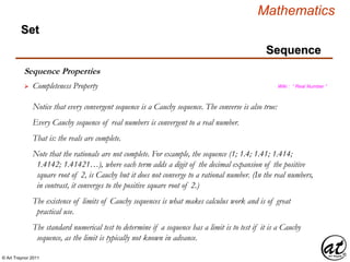
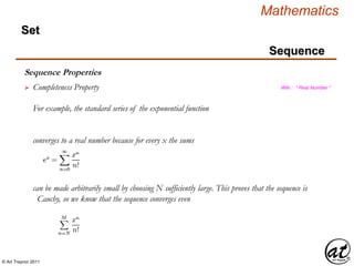
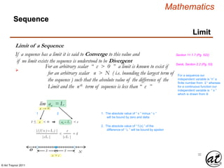
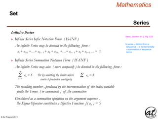
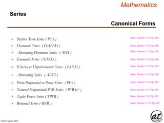
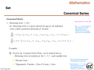
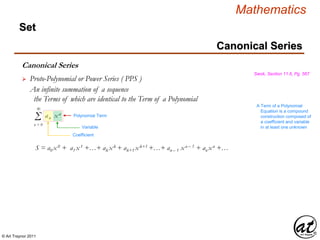
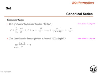
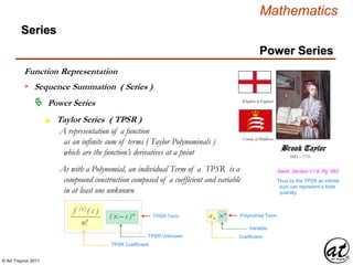
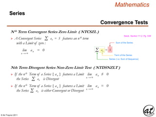
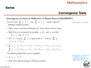
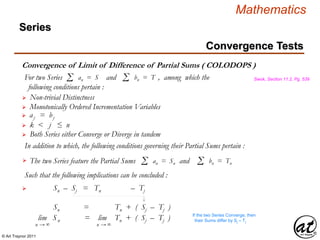
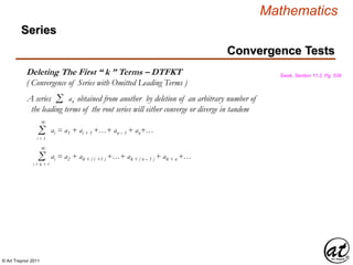
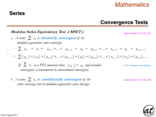
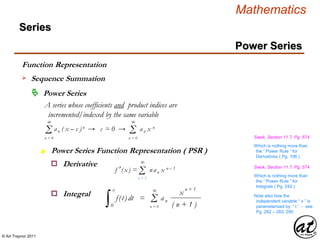
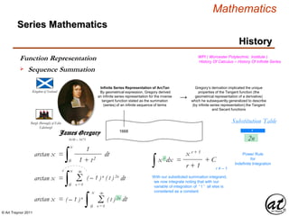
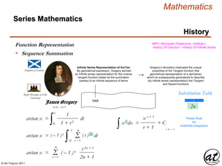
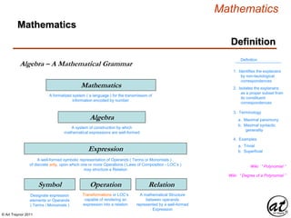
This document defines key mathematical concepts such as expressions, equations, polynomials, and their properties. It discusses:
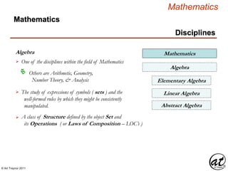
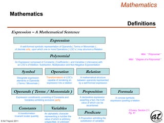
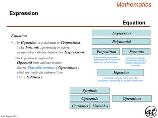
1) Mathematical expressions as well-formed symbolic representations composed of operands, operations, and relations.
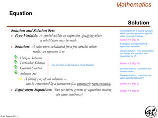
2) Equations as propositions expressing an equality relationship between expressions. Solutions are values substituted for free variables that render an equation true.
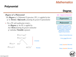
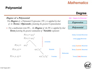
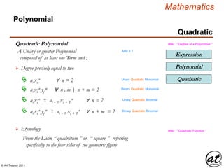
3) Polynomials as expressions composed of coefficients and variables, with operations including addition, subtraction, multiplication, and non-negative exponentiation. The degree of a polynomial is determined by the greatest exponent.

![© Art Traynor 2011
Mathematics
Definitions
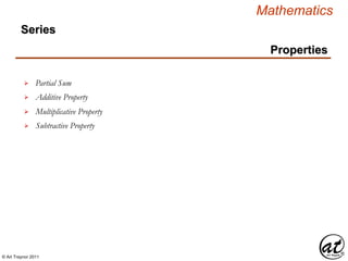
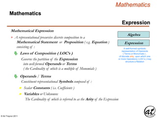
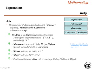
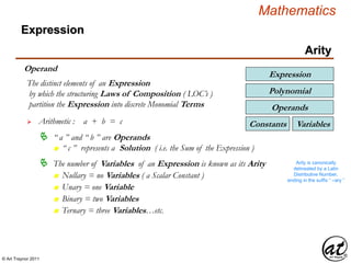
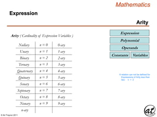
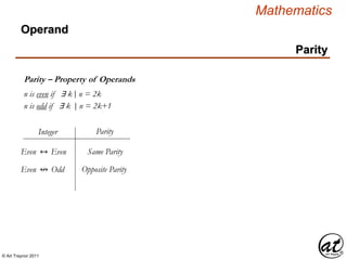
Expression
Symbol Operation Relation
Expression – A Mathematical Sentence
Proposition Formula
VariablesConstants
Operands ( Terms )
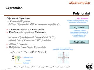
Equation
A formula stating an
equivalency class relation
Linear Equation
An equation in which each term is either
a constant or the product of a constant
and (a) variable[s] of the first degree
Mathematics
Polynomial](https://image.slidesharecdn.com/c9e9311b-9a34-4ce2-ba4a-c45da4ad39e4-160620060559/85/SequencesAndSeries_160505_01b-6-320.jpg)
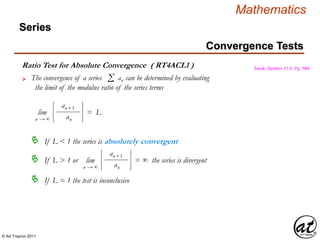
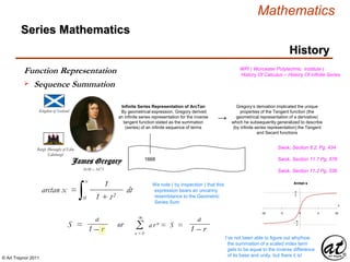
![© Art Traynor 2011
Mathematics
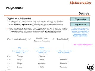
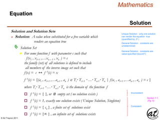
Linear Equation
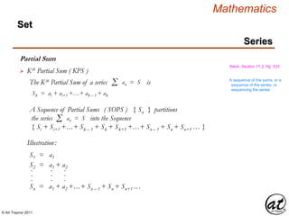
Linear Equation
Equation
An Equation consisting of:
Operands that are either
Any Variables are restricted to the First Order n = 1
Linear Equation
An equation in which each term
is either a constant or the
product of a constant and (a)
variable[s] of the first order
Expression
Proposition
Equation
Formula
n Constant(s) or
n A product of Constant(s) and
one or more Variable(s)
The Linear character of the Equation derives from the
geometry of its graph which is a line in the R2 plane
As a Relation the Arity of a Linear Equation must be
at least two, or n ≥ 2 , or a Binomial or greater Polynomial
Polynomial](https://image.slidesharecdn.com/c9e9311b-9a34-4ce2-ba4a-c45da4ad39e4-160620060559/85/SequencesAndSeries_160505_01b-21-320.jpg)
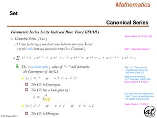
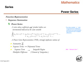
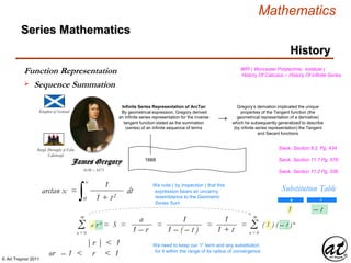
![© Art Traynor 2011
Mathematics
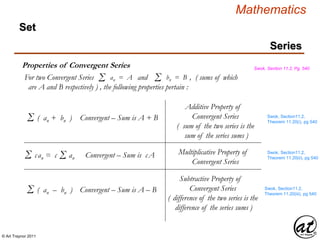
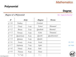
Equation
Linear Equation
Linear Equation
An equation in which each term is either a constant or the product
of a constant and (a) variable[s] of the first order
Term ai represents a Coefficient
b = Σi= 1
n
ai xi = ai xi + ai+1 xi+1…+ an – 1 xn – 1 + an xn
Equation of a Line in n-variables
A linear equation in “ n ” variables, xi + xi+1 …+ xn-1 + xn
has the form:
n Coefficients are distributed over a defined field
(e.g. ℕ , ℤ , ℚ , ℝ , ℂ )
Term xi represents a Variable ( e.g. x, y, z )
n Term a1 is defined as the Leading Coefficient
n Term x1 is defined as the Leading Variable
Section 1.1, (Pg. 2)
Section 1.1, (Pg. 2)
Section 1.1, (Pg. 2)
Section 1.1, (Pg. 2)
Coefficient = a multiplicative factor
(scalar) of fixed value (constant)
Section 1.1, (Pg. 2)](https://image.slidesharecdn.com/c9e9311b-9a34-4ce2-ba4a-c45da4ad39e4-160620060559/85/SequencesAndSeries_160505_01b-22-320.jpg)
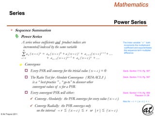
![© Art Traynor 2011
Mathematics
Linear Equation
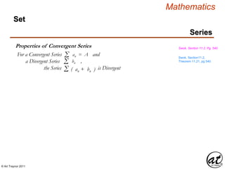
Equation
Standard Form ( Polynomial )
Ax + By = C
Ax1 + By1 = C
For the equation to describe a line ( no curvature )
the variable indices must equal one
ai xi + ai+1 xi+1 …+ an – 1 xn –1 + an xn = b
ai xi
1 + ai+1 x 1 …+ an – 1 x 1 + a1 x 1 = bi+1 n – 1 n n
ℝ
2
: a1 x + a2 y = b
ℝ
3
: a1 x + a2 y + a3 z = b
Blitzer, Section 3.2, (Pg. 226)
Section 1.1, (Pg. 2)
Test for Linearity
A Linear Equation can be expressed in Standard Form
As a species of Polynomial , a Linear Equation
can be expressed in Standard Form
Every Variable term must be of precise order n = 1
Linear Equation
An equation in which each term
is either a constant or the
product of a constant and (a)
variable[s] of the first order
Expression
Proposition
Equation
Formula
Polynomial](https://image.slidesharecdn.com/c9e9311b-9a34-4ce2-ba4a-c45da4ad39e4-160620060559/85/SequencesAndSeries_160505_01b-23-320.jpg)
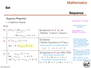
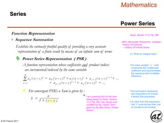
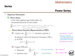
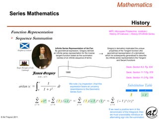
![© Art Traynor 2011
Mathematics
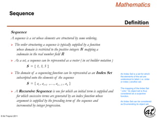
Sequence
A collection of real numbers that stands
in one-to-one correspondence with the set of positive integers. Swok, Section 11.1, (Pg. 520)
A set whose elements are structured by some ordering.
An Ordered Set
Wiki / AT: “ Sequence ”
A Function f
the domain of which is the set of positive integers. A Function
To each positive Integer “ k ” ,
there corresponds a Real Number “ f( k ) ”
f : ℤ + → ℝ , dom ( S ) = { k , n ℤ + | [ ak , ak+1 , … , an – 1 , an ] }
ran ( S ) = { k , n ℤ + | [ f(k) , f(k+1) , … , f(n – 1) , f(n) ] }
f(k) = ak → ℤ + x ℝ → ( k , ak ) , ( k +1 , ak+1 ) , … The Cartesian Product
… , ( n – 1, an – 1 ) , ( n , an )
Not necessarily a Sum (as is
the case with a Series)
The Cartesian Product
Definition
Sequence](https://image.slidesharecdn.com/c9e9311b-9a34-4ce2-ba4a-c45da4ad39e4-160620060559/85/SequencesAndSeries_160505_01b-25-320.jpg)