presentation calibration

1. UC: Calibrating instrumentation
and control devices

2. Why calibration
Calibration is essential to improving a company’s bottom line, by minimizing risk to
product defects and recalls, and enhancing a reputation for consistent quality.
Instrument calibration is a very important consideration in measurement systems.
All instruments suffer drift in their characteristics, and the rate at which this
happens depends on many factors, such as the environmental conditions in which
instruments are used and the frequency of their use. Thus, errors due to
instruments being out of calibration can usually be rectified by increasing the
frequency of recalibration.
Calibration can be an insurance policy because out-of-tolerance (OOT)
instruments may give false information leading to unreliable products, customer
dissatisfaction and increased warranty costs.
In addition, OOT conditions may cause good products to fail tests, which ultimately
results in unnecessary rework costs and production delays.

3. What is Calibration?
Calibration is the comparison of a measurement device (an unknown)
against an equal or better standard. A standard in a measurement is
considered the reference; it is the one in the comparison taken to be the more
correct of the two. Calibration finds out how far the unknown is from the standard.
Calibration is the act or result of quantitative comparison between a known standard
and the output of the measuring system. If the output-input response of the system
is linear, then a single-point calibration is sufficient. However, if the system
response is non-linear, then a set of known standard inputs to the measuring
system are employed for calibrating the corresponding outputs of the system.
A “typical” commercial calibration uses the manufacturer’s calibration
procedure and is performed with a reference standard at least four times more
accurate than the instrument under test.

4. Some Calibration Terms
• As found data—The reading of the instrument before it is adjusted.
• As left data—The reading of the instrument after adjustment or “same as
found,” if no adjustment was made.
• Optimization—Adjusting a measuring instrument to make it more accurate is
NOT part of a typical calibration and is frequently referred to as “optimizing” or
“nominalizing” an instrument.
• Out-of-tolerance (OOT) condition—When an instrument’s performance is
outside its specifications, it is considered an out of-tolerance (OOT) condition,
resulting in the need to adjust the instrument back into specification.
• Test uncertainty ratio (TUR)—This is the ratio of the accuracy of the
instrument under test compared to the accuracy of the reference standard.

5. Calibration and ranging
• Every instrument has at least one input and one output.
• To calibrate an instrument means to check and adjust (if necessary) its
response so the output accurately corresponds to its input
throughout a specified range
• In order to do this, one must expose the instrument to an actual input
stimulus of precisely known quantity.
• Eg. For a pressure gauge, indicator, or transmitter, this would mean
subjecting the pressure instrument to known fluid pressures and
comparing the instrument response against those known pressure
quantities.

6. • One cannot perform a true calibration without comparing an instrument’s
response to known.
• setting the lower and upper range values of an instrument to respond with the
desired sensitivity to changes in input is called ranging.
• For example, a pressure transmitter set to a range of 0 to 200 PSI (0 PSI = 4 mA
output ; 200 PSI = 20 mA output) could be re-ranged to respond on a scale of 0
to 150 PSI (0 PSI = 4 mA ; 150 PSI = 20 mA).
• so Calibration and ranging are two tasks associated with establishing an accurate
correspondence between any instrument’s input signal and its output signal.
• In analog instruments, re-ranging could (usually) only be accomplished by re-
calibration, since the same adjustments were used to achieve both purposes.
• In digital instruments, calibration and ranging are typically separate adjustments
(i.e. it is possible to re-range a digital transmitter without having to perform a
complete recalibration

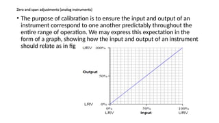
7. Zero and span adjustments (analog instruments)
• The purpose of calibration is to ensure the input and output of an
instrument correspond to one another predictably throughout the
entire range of operation. We may express this expectation in the
form of a graph, showing how the input and output of an instrument
should relate as in fig

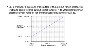
8. • Eg. a graph for a pressure transmitter with an input range of 0 to 100
(PSI) and an electronic output signal range of 4 to 20 milliamps (mA)
electric current relation for linear pressure transmitter will be.

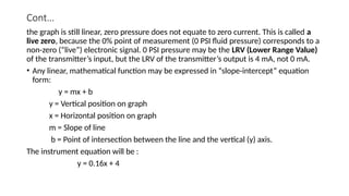
9. Cont…
the graph is still linear, zero pressure does not equate to zero current. This is called a
live zero, because the 0% point of measurement (0 PSI fluid pressure) corresponds to a
non-zero (“live”) electronic signal. 0 PSI pressure may be the LRV (Lower Range Value)
of the transmitter’s input, but the LRV of the transmitter’s output is 4 mA, not 0 mA.
• Any linear, mathematical function may be expressed in “slope-intercept” equation
form:
y = mx + b
y = Vertical position on graph
x = Horizontal position on graph
m = Slope of line
b = Point of intersection between the line and the vertical (y) axis.
The instrument equation will be :
y = 0.16x + 4

10. Cont…
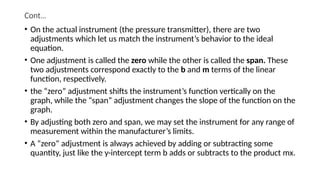
• On the actual instrument (the pressure transmitter), there are two
adjustments which let us match the instrument’s behavior to the ideal
equation.
• One adjustment is called the zero while the other is called the span. These
two adjustments correspond exactly to the b and m terms of the linear
function, respectively.
• the “zero” adjustment shifts the instrument’s function vertically on the
graph, while the “span” adjustment changes the slope of the function on the
graph.
• By adjusting both zero and span, we may set the instrument for any range of
measurement within the manufacturer’s limits.
• A “zero” adjustment is always achieved by adding or subtracting some
quantity, just like the y-intercept term b adds or subtracts to the product mx.

11. cont…
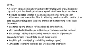
• A “span” adjustment is always achieved by multiplying or dividing some
quantity, just like the slope m forms a product with our input variable x.
• It should be noted that for most analog instruments, zero and span
adjustments are interactive. That is, adjusting one has an effect on the other.
Zero adjustments typically take one or more of the following forms in an
instrument:
• Bias force (spring or mass force applied to a mechanism)
• Mechanical offset (adding or subtracting a certain amount of motion)
• Bias voltage (adding or subtracting a certain amount of potential)
Span adjustments typically take one of these forms:
• Amplifier gain (multiplying or dividing a voltage signal)
• Spring rate (changing the force per unit distance of stretch)

12. Sensor calibration
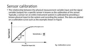
• The relationship between the physical measurement variable input and the signal
variable (output) for a specific sensor is known as the calibration of the sensor.
Typically, a sensor (or an entire instrument system) is calibrated by providing a
known physical input to the system and recording the output. The data are plotted
on a calibration curve such as the example shown in Figure
fig. Calibration curve

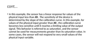
13. cont…
• In this example, the sensor has a linear response for values of the
physical input less than X0 . The sensitivity of the device is
determined by the slope of the calibration curve. In this example, for
values of the physical input greater than X0 , the calibration curve
becomes less sensitive until it reaches a limiting value of the output
signal. This behavior is referred to as saturation, and the sensor
cannot be used for measurements greater than its saturation value. In
some cases, the sensor will not respond to very small values of the
physical input variable.

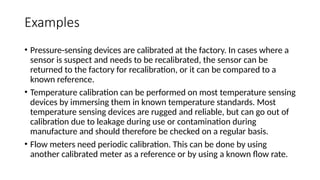
14. Examples
• Pressure-sensing devices are calibrated at the factory. In cases where a
sensor is suspect and needs to be recalibrated, the sensor can be
returned to the factory for recalibration, or it can be compared to a
known reference.
• Temperature calibration can be performed on most temperature sensing
devices by immersing them in known temperature standards. Most
temperature sensing devices are rugged and reliable, but can go out of
calibration due to leakage during use or contamination during
manufacture and should therefore be checked on a regular basis.
• Flow meters need periodic calibration. This can be done by using
another calibrated meter as a reference or by using a known flow rate.

15. Calibration procedures
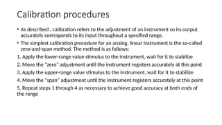
• As described , calibration refers to the adjustment of an instrument so its output
accurately corresponds to its input throughout a specified range.
• The simplest calibration procedure for an analog, linear instrument is the so-called
zero-and-span method. The method is as follows:
1. Apply the lower-range value stimulus to the instrument, wait for it to stabilize
2. Move the “zero” adjustment until the instrument registers accurately at this point
3. Apply the upper-range value stimulus to the instrument, wait for it to stabilize
4. Move the “span” adjustment until the instrument registers accurately at this point
5. Repeat steps 1 through 4 as necessary to achieve good accuracy at both ends of
the range

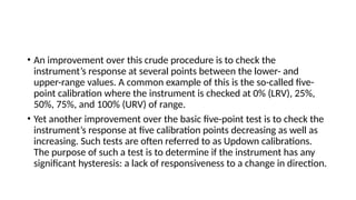
16. • An improvement over this crude procedure is to check the
instrument’s response at several points between the lower- and
upper-range values. A common example of this is the so-called five-
point calibration where the instrument is checked at 0% (LRV), 25%,
50%, 75%, and 100% (URV) of range.
• Yet another improvement over the basic five-point test is to check the
instrument’s response at five calibration points decreasing as well as
increasing. Such tests are often referred to as Updown calibrations.
The purpose of such a test is to determine if the instrument has any
significant hysteresis: a lack of responsiveness to a change in direction.

17. Calibration Intervals
• Time between any two calibrations of measuring and test instruments is known as
the calibration interval and must be established and monitored by the user in
accordance with his own requirements.
• Essential criteria for determining the calibration interval include:
The required accuracy vs. the instrument’s accuracy,
The impact an OOT will have on processes
The performance history of the particular instrument in its
application
The extent to which the measuring and test equipment is subject to stressing
Frequency of use
Ambient conditions
Stability of previous calibrations
Company-specific requirements specified by the quality assurance system

18. Calibration/trimming
(Digital instruments )
• The advent of “smart” field instruments containing
microprocessors has been a great advance for industrial
instrumentation. These devices have built-in diagnostic
ability, greater accuracy (due to digital compensation of
sensor nonlinearities), and the ability to communicate
digitally with host devices for reporting of various
parameters.
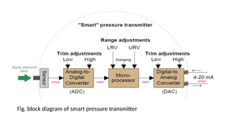
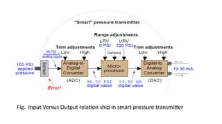
• A simplified block diagram of a “smart” pressure transmitter
looks something like this:

19. Fig. block diagram of smart pressure transmitter

20. Cont…
• . Not only can we set lower and upper-range values (LRV and URV) in
a smart transmitter, but it is also possible to calibrate the analog-to-
digital and digital-to-analog converter circuits independently of each
other.
• What this means for the calibration technician is that a full calibration
procedure on a smart transmitter potentially requires more work and
a greater number of adjustments than an all-analog transmitter.
• Just because you digitally set the LRV of a pressure transmitter to 0.00
PSI and the URV to 100.00 PSI does not necessarily mean it will
register accurately at points within that range! The following example
will illustrate this fallacy.

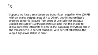
21. Eg.
• Suppose we have a smart pressure transmitter ranged for 0 to 100 PSI
with an analog output range of 4 to 20 mA, but this transmitter’s
pressure sensor is fatigued from years of use such that an actual
applied pressure of 100 PSI generates a signal that the analog-to-
digital converter interprets as only 96 PSI. Assuming everything else in
the transmitter is in perfect condition, with perfect calibration, the
output signal will still be in error:

22. Fig. Input Versus Output relation ship in smart pressure transmitter

23. Cont…
• The microprocessor “thinks” the applied pressure is only 96 PSI, and it
responds accordingly with a 19.36 mA output signal. The only way
anyone would ever know this transmitter was inaccurate at 100 PSI is to
actually apply a known value of 100 PSI fluid pressure to the sensor and
note the incorrect response.
• It is clear that digitally setting a smart instrument’s LRV and URV points
does not constitute a legitimate calibration of the instrument.
• For this reason, smart instruments always provide a means to perform
what is called a digital trim on both the ADC and DAC circuits, to ensure
the microprocessor “sees” the correct representation of the applied
stimulus and to ensure the microprocessor’s output signal gets
accurately converted into a DC current, respectively.

24. Cont…
• A convenient way to test a digital transmitter’s analog/digital
converters is to monitor the microprocessor’s process variable (PV)
and analog output (AO) registers while comparing the real input and
output values against trusted calibration standards. A HART
communicator device provides this “internal view” of the registers so
we may see what the microprocessor “sees.”
• The following example shows a differential pressure transmitter with
a sensor (analog-to-digital) calibration error

25. Eg.

26. Cont…
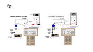
• Here in Fig a, the calibration standard for pressure input to the transmitter is a digital
pressure gauge, registering 25.00 inches of water column. The digital multimeter (DMM) is
our calibration standard for the current output, and it registers 11.93 milliamps. Since we
would expect an output of 12.00 milliamps at this pressure (given the transmitter’s range
values of 0 to 50 inches W.C.)
• we immediately know from the pressure gauge and multimeter readings that
some sort of calibration error exists in this transmitter. Comparing the HART
communicator’s displays of PV and AO against our calibration standards reveals
more information about the nature of this error.
• we see that the AO value (11.930 mA) agrees with the multimeter while the PV
value (24.781 ”W.C.) does not agree with the digital pressure gauge. This tells us
the calibration error lies within the sensor (input) of the transmitter and not
with the DAC (output). Thus, the correct calibration procedure to perform on
this errant transmitter is a sensor trim.

27. Cont…
• In Fig b, we see what an output (DAC) error would look like with another differential
pressure transmitter subjected to the same test.
• Once again, the calibration standard for pressure input to the transmitter is a digital
pressure gauge, registering 25.00 inches of water column. A digital multimeter (DMM)
still serves as our calibration standard for the current out put, and it registers 11.93
milliamps. Since we expect 12.00 milliamps output at this pressure (given the
transmitter’s range values of 0 to 50 inches W.C.),
• we immediately know from the pressure gauge and multimeter readings that some sort
of calibration error exists in this transmitter (just as before).
• Comparing the HART communicator’s displays of PV and AO against our calibration
standards reveals more information about the nature of this error: we see that the PV
value (25.002 inches W.C.) agrees with the digital pressure gauge while the AO value
(12.001 mA) does not agree with the digital multimeter. This tells us the calibration error
lies within the digital-to-analog converter (DAC) of the transmitter and not with the
sensor (input). Thus, the correct calibration procedure to perform on this errant
transmitter is an output trim.

28. Conclusion
• Merely comparing the pressure and current standards’ indications was not enough to tell
us any more than the fact we had some sort of calibration error inside the transmitter.
Not until we viewed the microprocessor’s own values of PV and AO could we determine
whether the calibration error was related to the ADC (input), the DAC (output), or
perhaps even both.
• Note how in both scenarios it was absolutely necessary to interrogate the transmitter’s
microprocessor registers with a HART communicator to determine where the error was
located.
• Once digital trims have been performed on both input and output converters, of course,
the technician is free to re-range the microprocessor as many times as desired without re-
calibration.
• An instrument technician may use a hand-held HART communicator device to re-set the
LRV and URV range values to whatever new values are desired by operations staff without
having to re-check calibration by applying known physical stimuli to the instrument. So
long as the ADC and DAC trims are both fine, the overall accuracy of the instrument will
still be good with the new range.

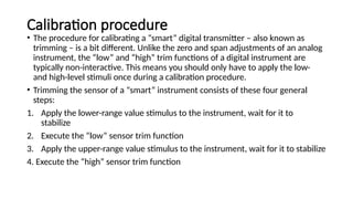
29. Calibration procedure
• The procedure for calibrating a “smart” digital transmitter – also known as
trimming – is a bit different. Unlike the zero and span adjustments of an analog
instrument, the “low” and “high” trim functions of a digital instrument are
typically non-interactive. This means you should only have to apply the low-
and high-level stimuli once during a calibration procedure.
• Trimming the sensor of a “smart” instrument consists of these four general
steps:
1. Apply the lower-range value stimulus to the instrument, wait for it to
stabilize
2. Execute the “low” sensor trim function
3. Apply the upper-range value stimulus to the instrument, wait for it to stabilize
4. Execute the “high” sensor trim function

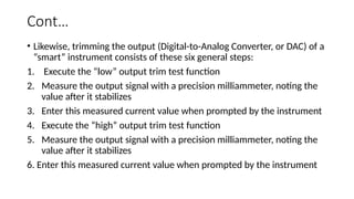
30. Cont…
• Likewise, trimming the output (Digital-to-Analog Converter, or DAC) of a
“smart” instrument consists of these six general steps:
1. Execute the “low” output trim test function
2. Measure the output signal with a precision milliammeter, noting the
value after it stabilizes
3. Enter this measured current value when prompted by the instrument
4. Execute the “high” output trim test function
5. Measure the output signal with a precision milliammeter, noting the
value after it stabilizes
6. Enter this measured current value when prompted by the instrument

31. Cont…
• After both the input and output (ADC and DAC) of a smart
transmitter have been trimmed (i.e. calibrated against standard
references known to be accurate), the lower- and upper-range values
may be set. In fact, once the trim procedures are complete, the
transmitter may be ranged and ranged again as many times as
desired. The only reason for re-trimming a smart transmitter is to
ensure accuracy over long periods of time where the sensor and/or
the converter circuitry may have drifted out of acceptable limits.