Measurments Basic Concepts pdf

1. Basic Concepts of
Measurement Methods
2141-375
Measurement and Instrumentation

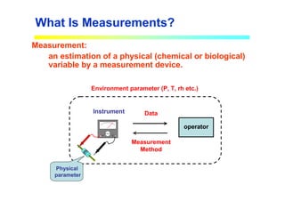
2. What Is Measurements?
Measurement:
an estimation of a physical (chemical or biological)
variable by a measurement device.
Instrument
Environment parameter (P, T, rh etc.)
Measurement
Method
V C
V C
operator
Data
Physical
parameter

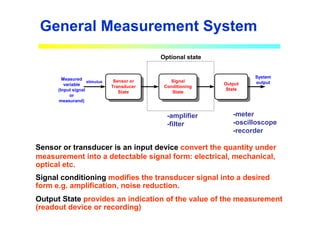
3. General Measurement System
-amplifier
-filter
-meter
-oscilloscope
-recorder
Sensor or
Transducer
State
Signal
Conditioning
State
Output
State
Measured
variable
(Input signal
or
measurand)
stimulus
System
output
Optional state
Sensor or transducer is an input device convert the quantity under
measurement into a detectable signal form: electrical, mechanical,
optical etc.
Signal conditioning modifies the transducer signal into a desired
form e.g. amplification, noise reduction.
Output State provides an indication of the value of the measurement
(readout device or recording)

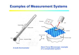
4. Examples of Measurement Systems
A bulb thermometer
Atom Force Microscope: example
of a complicated system

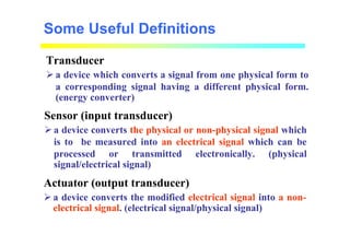
5. Transducer
a device which converts a signal from one physical form to
a corresponding signal having a different physical form.
(energy converter)
Sensor (input transducer)
a device converts the physical or non-physical signal which
is to be measured into an electrical signal which can be
processed or transmitted electronically. (physical
signal/electrical signal)
Actuator (output transducer)
a device converts the modified electrical signal into a non-
electrical signal. (electrical signal/physical signal)
Some Useful Definitions

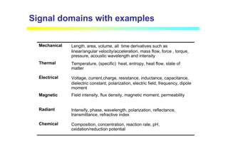
6. Composition, concentration, reaction rate, pH,
oxidation/reduction potential
Chemical
Intensify, phase, wavelength, polarization, reflectance,
transmittance, refractive index
Radiant
Field intensity, flux density, magnetic moment, permeability
Magnetic
Voltage, current,charge, resistance, inductance, capacitance,
dielectric constant, polarization, electric field, frequency, dipole
moment
Electrical
Temperature, (specific) heat, entropy, heat flow, state of
matter
Thermal
Length, area, volume, all time derivatives such as
linear/angular velocity/acceleration, mass flow, force , torque,
pressure, acoustic wavelength and intensity
Mechanical
Signal domains with examples

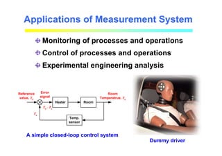
7. Applications of Measurement System
Monitoring of processes and operations
Control of processes and operations
Experimental engineering analysis
A simple closed-loop control system
Heater Room
Temp.
sensor
Error
signal
Reference
value, Td
Ta
Td
- Ta
Room
Temperatrue, Ta
Dummy driver

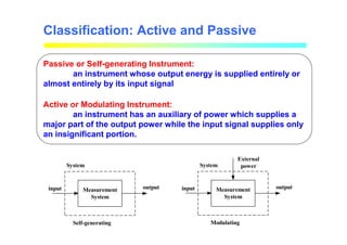
8. Classification: Active and Passive
Passive or Self-generating Instrument:
an instrument whose output energy is supplied entirely or
almost entirely by its input signal
Active or Modulating Instrument:
an instrument has an auxiliary of power which supplies a
major part of the output power while the input signal supplies only
an insignificant portion.
input output
System
Self-generating
Measurement
System
input output
System
Modulating
Measurement
System
External
power

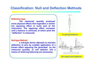
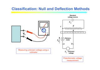
9. Classification: Null and Deflection Methods
Deflection-type
The measured quantity produced
some physical effects that engenders a similar
but opposing effect in some part of the
instrument. The opposing effect increases
until a balance is achieved, at which point the
“deflection” is measured.
Null-type Method:
a null-type device attempts to maintain
deflection at zero by suitable application of a
known effect opposing the generated by the
measured quantity. (a null detector and a
means of restoring balancing are necessary).
An equal arm balance
A spring balance

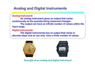
10. Analog and Digital Instruments
Digital Instruments:
The digital instruments has an output that varies in
discrete steps and so can only have a finite number of values.
Analog Instrument:
An analog instrument gives an output that varies
continuously as the quantity being measured changes.
The output can have an infinite number of values within the
input range.
Example of an analog and digital instrument

11. G
Galvano-
meter
a b
Vx
Unknown
voltage
Im
Standard
voltage source
VS
c d
Measuring unknown voltage using a
voltmeter
Potentiometer voltage
measurement
V
+ -
Vx
Vx
Classification: Null and Deflection Methods

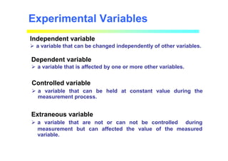
12. Experimental Variables
Independent variable
a variable that can be changed independently of other variables.
Dependent variable
a variable that is affected by one or more other variables.
Controlled variable
a variable that can be held at constant value during the
measurement process.
Extraneous variable
a variable that are not or can not be controlled during
measurement but can affected the value of the measured
variable.

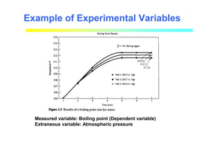
13. Example of Experimental Variables
Measured variable: Boiling point (Dependent variable)
Extraneous variable: Atmospheric pressure

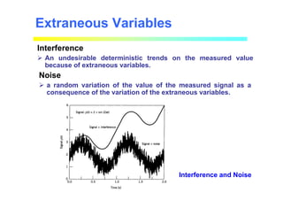
14. Extraneous Variables
Interference
An undesirable deterministic trends on the measured value
because of extraneous variables.
Noise
a random variation of the value of the measured signal as a
consequence of the variation of the extraneous variables.
Interference and Noise

15. Calibration
•Calibration:
A test in which known values of the input are applied to a
measurement system (or sensor) for the purpose of observing the
system (or sensor) output.
•Dynamic calibration:
When the variables of interest are time dependent and
time-based information is need. The dynamic calibration
determines the relationship between an input of known dynamic
behavior and the measurement system output.
•Static calibration:
A calibration procedure in which the values of the
variable involved remain constant (do not change with time).

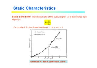
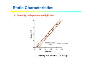
16. Static Characteristics
Static Sensitivity: Incremental ratio of the output signal (y) to the desired input
signal (x).
y
S
x
∆
=
∆
S = constant, If y is a linear function of x, i.e. y = ax + b
Example of Static calibration curve

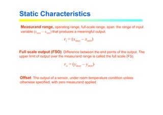
17. Measurand range, operating range, full-scale range, span: the range of input
variable (xmax – xmin) that produces a meaningful output.
Full scale output (FSO): Difference between the end points of the output. The
upper limit of output over the measurand range is called the full scale (FS)
Offset: The output of a sensor, under room temperature condition unless
otherwise specified, with zero measurand applied.
Static Characteristics
ri = (xmax – xmin)
ro = (ymax – ymin)

18. Static Characteristics
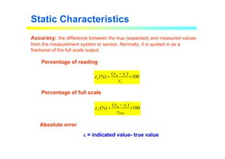
Accuracy: the difference between the true (expected) and measured values
from the measurement system or sensor. Normally, it is quoted in as a
fractional of the full scale output.
( )
(%) 100
m t
a
t
y y
y
ε
−
= ×
FSO
( )
(%) 100
m t
f
y y
y
ε
−
= ×
Percentage of reading
Percentage of full scale
Absolute error
ε
ε
ε
ε = indicated value- true value

19. Static Characteristics
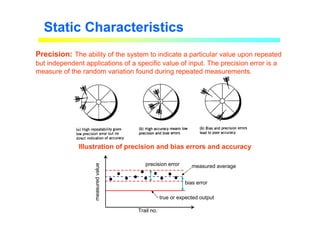
bias error
precision error
true or expected output
measured average
measured
value
Trail no.
Precision: The ability of the system to indicate a particular value upon repeated
but independent applications of a specific value of input. The precision error is a
measure of the random variation found during repeated measurements.
Illustration of precision and bias errors and accuracy

20. Static Characteristics
Load cell output
(mV)
Trail
no.
A B C
1 10.02 11.50 10.00
2 10.96 11.53 10.03
3 11.20 11.52 10.02
4 9.39 11.47 9.93
5 10.50 11.42 9.92
6 10.94 11.51 10.01
7 9.02 11.58 10.08
8 9.47 11.50 10.00
9 10.08 11.43 9.97
10 9.32 11.48 9.98
Maximum 11.20 11.58 10.08
Average 10.09 11.49 9.99
Minimum 9.02 11.42 9.92
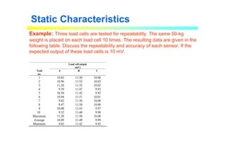
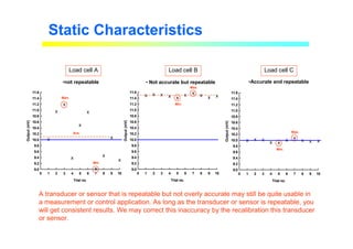
Example: Three load cells are tested for repeatability. The same 50-kg
weight is placed on each load cell 10 times. The resulting data are given in the
following table. Discuss the repeatability and accuracy of each sensor. If the
expected output of these load cells is 10 mV.

21. Static Characteristics
Trial no.
0 1 2 3 4 5 6 7 8 9 10
Output
(mV)
9.0
9.2
9.4
9.6
9.8
10.0
10.2
10.4
10.6
10.8
11.0
11.2
11.4
11.6
x
x
x
x
x
x
x
x
x
x
Trial no.
0 1 2 3 4 5 6 7 8 9 10
Output
(mV)
9.0
9.2
9.4
9.6
9.8
10.0
10.2
10.4
10.6
10.8
11.0
11.2
11.4
11.6
x x x x x
x x x x x
Trial no.
0 1 2 3 4 5 6 7 8 9 10
Output
(mV)
9.0
9.2
9.4
9.6
9.8
10.0
10.2
10.4
10.6
10.8
11.0
11.2
11.4
11.6
x x x
x x
x x x x x
Load cell A Load cell B Load cell C
Max.
Min
Ave.
Max.
Min.
Max.
Min.
•not repeatable • Not accurate but repeatable •Accurate and repeatable
A transducer or sensor that is repeatable but not overly accurate may still be quite usable in
a measurement or control application. As long as the transducer or sensor is repeatable, you
will get consistent results. We may correct this inaccuracy by the recalibration this transducer
or sensor.

22. Static Characteristics
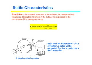
Resolution: the smallest increment in the value of the measurand that
results in a detectable increment in the output. It is expressed in the
percentage of the measurand range
max min
Resolution (%) 100
x
x x
∆
= ×
−
A simple optical encoder
Each time the shaft rotates ¼ of a
revolution, a pulse will be
generated. So, this encoder has a
90oC resolution.

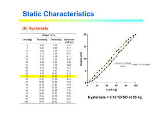
23. Static Characteristics
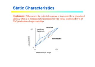
Hysteresis: Difference in the output of a sensor or instrument for a given input
value x, when x is increased and decreased or vice versa. (expressed in % of
FSO) (indication of reproducibility)
output
(%FSO)
measurand (% range)
0 100
0
100 maximum
hysteresis
upscale
downscale

24. Static Characteristics
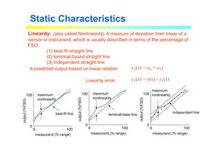
Linearity: (also called Nonlinearity) A measure of deviation from linear of a
sensor or instrument, which is usually described in terms of the percentage of
FSO.
(1) best-fit straight line
(2) terminal-based straight line
(3) independent straight line
output
(%FSO)
measurand (% range)
0 100
0
100 maximum
nonlinearity
terminal-base line
output
(%FSO)
measurand (% range)
0 100
0
100 maximum
nonlinearity
best-fit line
output
(%FSO)
measurand (% range)
0 100
0
100
maximum
nonlinearity
independent line
yL(x) = a0 + a1x
A predicted output based on linear relation:
Linearity error: eL(x) = y(x) - yL(x)

25. Static Characteristics
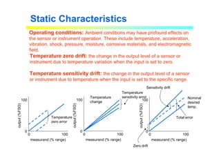
Operating conditions: Ambient conditions may have profound effects on
the sensor or instrument operation. These include temperature, acceleration,
vibration, shock, pressure, moisture, corrosive materials, and electromagnetic
field.
output
(%FSO)
measurand (% range)
0 100
0
100
Temperature
sensitivity error
Temperature
change
output
(%FSO)
measurand (% range)
0 100
0
100
Temperature
zero error
output
(%FSO) measurand (% range)
0 100
0
100
Zero drift
Sensitivity drift
Total error
Nominal
desired
temp.
Temperature zero drift: the change in the output level of a sensor or
instrument due to temperature variation when the input is set to zero.
Temperature sensitivity drift: the change in the output level of a sensor
or instrument due to temperature when the input is set to the specific range.

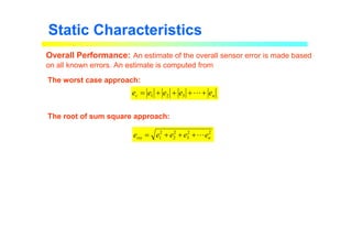
26. Overall Performance: An estimate of the overall sensor error is made based
on all known errors. An estimate is computed from
Static Characteristics
The worst case approach:
The root of sum square approach:
n
c e
e
e
e
e +
+
+
+
= L
3
2
1
2
2
3
2
2
2
1 n
rss e
e
e
e
e L
+
+
+
=

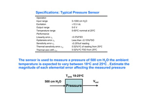
27. 0-1000 cm H2O
±15 V dc
0-5 V
0-50oC nominal at 25oC
±0.5%FSO
Less than ±0.15%FSO
±0.25%of reading
0.02%/oC of reading from 25oC
0.02%/oC FSO from 25oC
Operation
Input range
Excitation
Output range
Temperature range
Performance
Linearity error eL
Hysteresis error eh
Sensitivity error eS
Thermal sensitivity error eST
Thermal zero drift eZT
Specifications: Typical Pressure Sensor
The sensor is used to measure a pressure of 500 cm H2O the ambient
temperature is expected to vary between 18oC and 25oC . Estimate the
magnitude of each elemental error affecting the measured pressure
Pressure
500 cm H2O
Tamb 18-25oC
Vout

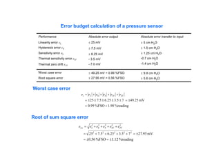
28. ± 9.9 cm H2O
± 5.6 cm H2O
± 49.25 mV = 0.99 %FSO
± 27.95 mV = 0.56 %FSO
Worst case error
Root square error
Absolute error output
± 25 mV
± 7.5 mV
± 6.25 mV
- 3.5 mV
- 7.0 mV
Absolute error transfer to input
± 5 cm H2O
± 1.5 cm H2O
± 1.25 cm H2O
-0.7 cm H2O
-1.4 cm H2O
Performance
Linearity error eL
Hysteresis error eh
Sensitivity error eS
Thermal sensitivity error eST
Thermal zero drift eZT
Error budget calculation of a pressure sensor
%reading
1.98
%FSO
0.99
mV
25
.
49
7
5
.
3
25
.
6
5
.
7
25
=
=
±
=
±
±
±
±
±
=
+
+
+
+
= ZT
ST
S
h
L
c e
e
e
e
e
e
%reading
1.12
%FSO
0.56
mV
95
.
27
7
5
.
3
25
.
6
5
.
7
25 2
2
2
2
2
2
2
2
2
2
±
=
±
=
±
=
+
+
+
+
=
+
+
+
+
= ZT
ST
S
h
L
rss e
e
e
e
e
e
Worst case error
Root of sum square error
1.25

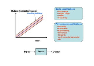
29. Performance specifications
• Accuracy
• Resolution
• Repeatability
• Hysteresis
• Linearity
• environmental parameter
• etc.
Confidential band
Output (Indicated value)
Input
Basic specifications
• Input range
• Output range
• Offset
• Sensitivity
Sensor
Input Output

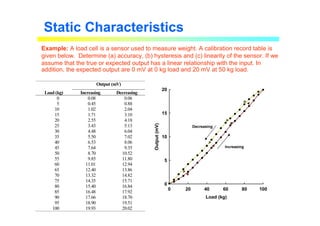
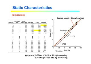
30. Static Characteristics
Example: A load cell is a sensor used to measure weight. A calibration record table is
given below. Determine (a) accuracy, (b) hysteresis and (c) linearity of the sensor. If we
assume that the true or expected output has a linear relationship with the input. In
addition, the expected output are 0 mV at 0 kg load and 20 mV at 50 kg load.
Output (mV)
Load (kg) Increasing Decreasing
0 0.08 0.06
5 0.45 0.88
10 1.02 2.04
15 1.71 3.10
20 2.55 4.18
25 3.43 5.13
30 4.48 6.04
35 5.50 7.02
40 6.53 8.06
45 7.64 9.35
50 8.70 10.52
55 9.85 11.80
60 11.01 12.94
65 12.40 13.86
70 13.32 14.82
75 14.35 15.71
80 15.40 16.84
85 16.48 17.92
90 17.66 18.70
95 18.90 19.51
100 19.93 20.02
Load (kg)
0 20 40 60 80 100
Output
(mV)
0
5
10
15
20
Increasing
Decreasing

31. Load (kg)
0 20 40 60 80 100
Output
(mV)
0
5
10
15
20
Increasing
Decreasing
Static Characteristics
(a) Accuracy
…
…
…
…
…
… %FSO
%reading
Desired output = 0.2mV/kg x load
Accuracy: %FSO = -7.85% at 25 kg increasing
%reading = -55% at 5 kg increasing
Load (kg)
True Output
(mV)
Actual
Output (mV) Error (mV) %FSO %reading
0 0 0.08 0.08 0.40 a
5 1 0.45 -0.55 -2.75 -55.00
10 2 1.02 -0.98 -4.90 -49.00
15 3 1.71 -1.29 -6.45 -43.00
20 4 2.55 -1.45 -7.25 -36.25
25 5 3.43 -1.57 -7.85 -31.40
30 6 4.48 -1.52 -7.60 -25.33
35 7 5.5 -1.50 -7.50 -21.43
40 8 8.06 0.06 0.30 0.75
35 7 7.02 0.02 0.10 0.29
30 6 6.04 0.04 0.20 0.67
25 5 5.13 0.13 0.65 2.60
20 4 4.18 0.18 0.90 4.50
15 3 3.1 0.10 0.50 3.33
10 2 2.04 0.04 0.20 2.00
5 1 0.88 -0.12 -0.60 -12.00
0 0 0.06 0.06 0.30 a

32. Static Characteristics
(b) Hysteresis
Load (kg)
0 20 40 60 80 100
Output
(mV)
0
5
10
15
20
Output (mV)
Load (kg) Increasing Decreasing Hysteresis
(%FSO)
0 0.08 0.06 0.10
5 0.45 0.88 2.15
10 1.02 2.04 5.10
15 1.71 3.10 6.95
20 2.55 4.18 8.15
25 3.43 5.13 8.50
30 4.48 6.04 7.80
35 5.50 7.02 7.60
40 6.53 8.06 7.65
45 7.64 9.35 8.55
50 8.70 10.52 9.10
55 9.85 11.80 9.75
60 11.01 12.94 9.65
65 12.40 13.86 7.30
70 13.32 14.82 7.50
75 14.35 15.71 6.80
80 15.40 16.84 7.20
85 16.48 17.92 7.20
90 17.66 18.70 5.20
95 18.90 19.51 3.05
100 19.93 20.02 0.45
%FSO
75
.
9
%
100
mV
20
mV
9.85
mV
11.80
=
×
−
Hysteresis = 9.75 %FSO at 55 kg

33. Load (kg)
0 20 40 60 80 100
Output
(mV)
0
5
10
15
20
endpoint
%FSO
85
.
7
%
100
mV
20
mV
00
.
5
mV
43
.
3
−
=
×
−
Static Characteristics
(c) Linearity: Terminal-based straight line (endpoint straight line)
endpoint
…
…
…
…
Linearity = -7.85 %FSO (at 25 kg)
Load (kg)
Endpoint
line (mV)
Actual Output
(mV)
Linearity
(%FSO)
0 0 0.08 0.40
5 1 0.45 -2.75
10 2 1.02 -4.90
15 3 1.71 -6.45
20 4 2.55 -7.25
25 5 3.43 -7.85
30 6 4.48 -7.60
35 7 5.50 -7.50
40 8 6.53 -7.35
y ~ 0.20 mV/kg x
40 8 8.06 -0.30
35 7 7.02 -0.10
30 6 6.04 -0.20
25 5 5.13 -0.65
20 4 4.18 -0.90
15 3 3.10 -0.50
10 2 2.04 -0.20
5 1 0.88 0.60
0 0 0.06 -0.30

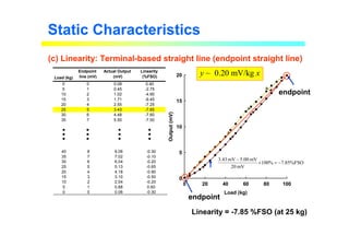
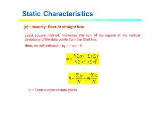
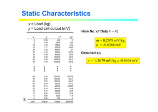
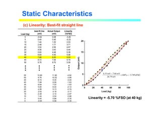
34. Static Characteristics
(c) Linearity: Best-fit straight line
Least square method: minimizes the sum of the square of the vertical
deviations of the data points from the fitted line.
Here, we will estimate y by y = mx + b
N = Total number of data points
( )2
2
x
x
N
y
x
xy
N
m
∑
−
∑
∑
∑
−
∑
=
N
x
m
N
y
b
∑
−
∑
=

35. Static Characteristics
45 9.35 2025.00 420.75
40 8.06 1600.00 322.4
35 7.02 1225.00 245.7
30 6.04 900.00 181.2
25 5.13 625.00 128.25
20 4.18 400.00 83.6
15 3.10 225.00 46.5
10 2.04 100.00 20.4
5 0.88 25.00 4.4
0 0.06 0.00 0
2100 409.89 143500 28499.45
x = Load (kg)
y = Load cell output (mV)
x y x xy
0 0.08 0.00 0
5 0.45 25.00 2.25
10 1.02 100.00 10.2
15 1.71 225.00 25.65
20 2.55 400.00 51
25 3.43 625.00 85.75
30 4.48 900.00 134.4
35 5.50 1225.00 192.5
40 6.53 1600.00 261.2
45 7.64 2025.00 343.8
50 8.70 2500.00 435
2
…
…
…
…
∑
∑
∑
∑
Here No. of Data N = 42
m = 0.2079 mV/kg
b = -0.6368 mV
y = 0.2079 mV/kg x -0.6368 mV
Obtained eq.

36. 60 11.84 12.94 -5.30
55 10.80 11.80 -4.82
50 9.76 10.52 -3.66
45 8.72 9.35 -3.04
40 7.68 8.06 -1.83
35 6.64 7.02 -1.83
30 5.60 6.04 -2.12
25 4.56 5.13 -2.74
20 3.52 4.18 -3.17
15 2.48 3.10 -2.97
10 1.44 2.04 -2.88
5 0.40 0.88 -2.30
0 -0.64 0.06 -3.35
%FSO
70
.
5
%
100
mV
20.15
mV
68
.
7
mV
.53
6
−
=
×
−
Static Characteristics
(c) Linearity: Best-fit straight line
…
…
…
…
Linearity = -5.70 %FSO (at 40 kg)
Load (kg)
0 20 40 60 80 100
Output
(mV)
0
5
10
15
20
%FSO
70
.
5
%
100
mV
20.79
mV
68
.
7
mV
.53
6
−
=
×
−
Load (kg)
best-fit line
(mV)
Actual Output
(mV)
Linearity
(%FSO)
0 -0.64 0.08 -3.45
5 0.40 0.45 -0.23
10 1.44 1.02 2.03
15 2.48 1.71 3.71
20 3.52 2.55 4.67
25 4.56 3.43 5.44
30 5.60 4.48 5.39
35 6.64 5.50 5.48
40 7.68 6.53 5.53
45 8.72 7.64 5.19
50 9.76 8.70 5.09
55 10.80 9.85 4.56

37. Load (kg)
0 20 40 60 80 100
Output
(mV)
0
5
10
15
20
%FSO
85
.
5
%
100
mV
20
mV
65
.
5
mV
48
.
4
−
=
×
−
Static Characteristics
(c) Linearity: Independent straight line
Linearity = -5.85 %FSO (at 30 kg)