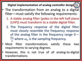
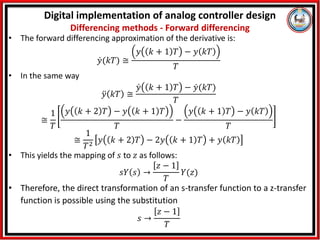
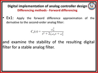
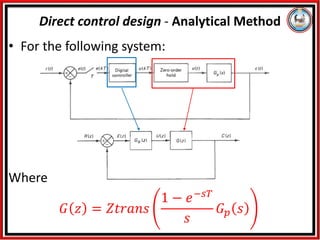
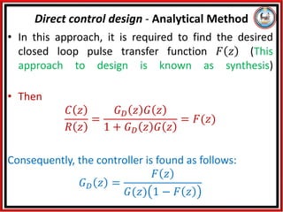
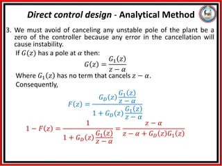
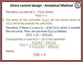
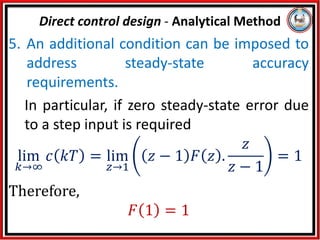
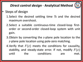
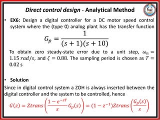
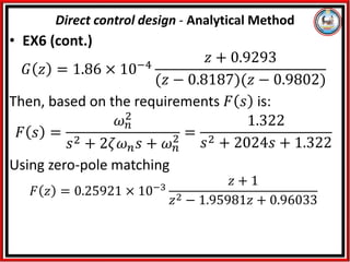
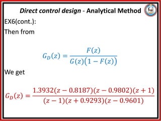
Lecture_8-Digital implementation of analog controller design.pdf

Digital implementation of Analog Controllers
Direct control design - Analytical Method
Dr. Amin Danial

References
❑ Katsuhiko Ogata Discrete-Time Control
Systems 2nd edition,1995
❑ M. Sami Fadali, Antonio Visioli - Digital
Control Engineering, Analysis and Design-
Second Edition_Academic Press (2019)
❑ Gene F. Franklin, J. David Powell, Michael L.
Workman - Digital Control of Dynamic
Systems-Prentice Hall (1998)
❑ A. V. OPPENHEIM, A. S. WILLSKY and S. H.
NAWAB , Signals & Systems, PRENTICE HALL,
1996.

Digital implementation of analog controller design
•This lecture introduces an indirect approach to digital
controller design.
•The approach is based on designing an analog controller
for the analog subsystem and then obtaining an
equivalent digital controller and using it to digitally
implement the desired control.
•The digital controller can be obtained using a number of
methods that are well known in the field of signal
processing, where they are used in the design of digital
filters.
•In fact, a controller can be viewed as a filter that
attenuates some dynamics and enhance others so as to
obtain the desired time response.

Procedure:
1. Design a controller 𝐶(𝑠) for the analog subsystem to
meet the desired design specifications.
2. Map the analog controller to a digital controller 𝐶(𝑧)
using a suitable transformation.
3. Tune the gain of the transfer function meet the design
specifications.
4. Check the sampled time response of the digital control
system and repeat steps 1 to 3, if necessary, until the
design specifications are met.

• The transformation from an analog to a digital
filter—must satisfy the following requirements:
1. A stable analog filter (poles in the left half plane
(LHP)) must transform to a stable digital filter.
2. The frequency response of the digital filter
must closely resemble the frequency response
of the analog filter in the frequency range 0 −
𝜔𝑠
2
where 𝜔𝑠 is the sampling frequency.
• Most filter transformations satisfy these two
requirements to varying degrees.
• However, this is not true of all analog-to-digital
transformations

• The forward differencing approximation of the derivative is:
ሶ
𝑦(𝑘𝑇) ≅
𝑦 𝑘 + 1 𝑇 − 𝑦 𝑘𝑇
𝑇
• In the same way
ሷ
𝑦 𝑘𝑇 ≅
ሶ
𝑦 𝑘 + 1 𝑇 − ሶ
𝑦(𝑘𝑇)
𝑇
≅
1
𝑇
𝑦 𝑘 + 2 𝑇 − 𝑦 𝑘 + 1 𝑇
𝑇
−
𝑦 𝑘 + 1 𝑇 − 𝑦 𝑘𝑇
𝑇
≅
1
𝑇2
𝑦 𝑘 + 2 𝑇 − 2𝑦 𝑘 + 1 𝑇 + 𝑦 𝑘𝑇
• This yields the mapping of 𝑠 to 𝑧 as follows:
𝑠𝑌 𝑠 →
𝑧 − 1
𝑇
𝑌(𝑧)
• Therefore, the direct transformation of an s-transfer function to a z-transfer
function is possible using the substitution
𝑠 →
𝑧 − 1
𝑇
Differencing methods - Forward differencing

• Ex1: Apply the forward difference approximation of the
derivative to the second-order analog filter:
and examine the stability of the resulting digital
filter for a stable analog filter.

• EX1(Cont.): Solution: (Note 𝑦(𝑘𝑇) ≡ 𝑦(𝑘))
• The differential equation from the given transfer function is:
• Then
• By multiply both sides by 𝑇2and rearrange the equation
• Equivalently, we obtain the transfer function of the filter using the
simpler transformation

• EX1(Cont.): Solution:
• For a stable analog filter, we have 𝜁 > 0 and 𝜔𝑛 > 0
(positive denominator coefficients are sufficient for a
second-order polynomial)
• From Jury test, the instability condition 𝑎𝑛 > 𝑎0 :
• If the sampling period of 0.2 s and an undamped natural
frequency of 10 rad/s yield unstable filters for any
underdamped analog filter.

• The backward differencing approximation of the derivative is:
(Note 𝑦(𝑘𝑇) ≡ 𝑦(𝑘))
• Similarly
• This yields the substitution
Differencing methods - Backward differencing

• Ex2: Apply the backward difference approximation of the
derivative to the second-order analog filter.
and examine the stability of the resulting digital filter for a stable
analog filter.
Solution:

• Ex2: (cont.)
• The stability conditions for the digital filter (Jury test) are
• The conditions are all satisfied for 𝜁 > 0 and 𝜔𝑛 > 0—that is, for
all stable analog filters.
𝑎𝑛 < 𝑎0 →
𝑃 1 > 0 →
𝑃 −1 > 0 →

• In pole-zero matching, a discrete approximation is obtained from an
analog filter by mapping both poles and zeros using 𝑃𝑠 = 𝑒𝑃𝑠𝑇
or
𝑃𝑧 = 𝑒𝑃𝑧𝑇
, where 𝑃𝑠 or 𝑃𝑧 is a pole or a zero in the z-domain and the
s-domain, respectively.
• If the analog filter has 𝑛 poles and 𝑚 zeros, then we say that the
filter has 𝑛 − 𝑚 zeros at infinity.
• For 𝑛 − 𝑚 zeros at infinity, we add 𝑛 − 𝑚 − 1 digital filter zeros at
− 1. Leading to the computation of the output requires values of the
input at past sampling points
• If the zeros are not added, it can be shown that the resulting system
will include a time delay.
• Finally, we adjust the gain of the digital filter so that it is equal to that
of the analog filter at a critical frequency dependent on the filter. For
a low-pass filter, 𝛼 is selected so that the gains are equal at DC; for a
bandpass filter, they are set equal at the center of the pass band.
Pole-zero matching

• For analog filter:
𝐺𝑎 𝑠 = 𝐾
ς𝑖=1
𝑚
(𝑠 − 𝑎𝑖)
ς𝑗=1
𝑛
(𝑠 − 𝑏𝑗)
• We get the corresponding digital filter as follows:
𝐺 𝑧 = 𝛼𝐾
𝑧 + 1 𝑛−𝑚−1 ς𝑖=1
𝑚
(𝑧 − 𝑒𝑎𝑖𝑇)
ς𝑗=1
𝑛
(𝑧 − 𝑒𝑏𝑗𝑇
)
• Where α is a constant selected for equal filter gains at a critical
frequency. For example, for a low-pass filter, α is selected to match
the DC gains using 𝐺 1 = 𝐺𝑎(0).
• For a high-pass filter, it is selected to match the high-frequency
gains using 𝐺 −1 = 𝐺𝑎 ∞ (Setting 𝑧 = 𝑒 𝑗𝜔𝑇 = −1 (i.e., 𝜔𝑇 =
𝜋) is equivalent to selecting the folding frequency 𝜔𝑠/2, which is
the highest frequency allowable without aliasing)
Pole-zero matching

• Ex3: Find a pole-zero matched digital filter
approximation for the analog filter.
If the damping ratio is equal to 0.5 and the undamped
natural frequency is 5 rad/s, determine the transfer
function of the digital filter for a sampling period of 0.1 s.
Pole-zero matching

Ex3: (cont.) Solution
• The analog filter has two zeros at infinity and complex conjugate
poles at 𝑠 = −𝜁𝜔𝑛 ± 𝑗𝜔𝑑.
• using the pole-zero matching transformation we get
𝐺 𝑧 = 𝛼
𝑧 + 1
𝑧 − 𝑒−𝜁𝜔𝑛𝑇𝑒𝑗𝜔𝑑𝑇 ( 𝑧 − 𝑒−𝜁𝜔𝑛𝑇𝑒−𝑗𝜔𝑑𝑇
𝐺 𝑧 = 𝛼
𝑧 + 1
𝑧2 − 2𝑒−𝜁𝜔𝑛𝑇 cos 𝜔𝑑𝑇 + 𝑒−2𝜁𝜔𝑛𝑇
For 𝜁 = 0.5, 𝜔𝑛 = 5, 𝑎𝑛𝑑 𝑇 = 0.1. then 𝜔𝑑 = 𝜔𝑛 1 − 𝜁2, the gain 𝛼
is determined from 𝐺 1 = 𝐺𝑎 0
Therefore,
𝐺 𝑧 =
0.0963(𝑧 + 1)
𝑧2 − 1.414𝑧 + 0.6065
Pole-zero matching

• Using the relation :
𝑧 = 𝑒𝑠𝑇
=
𝑒
𝑠𝑇
2
𝑒−
𝑠𝑇
2
≅
1 +
𝑠𝑇
2
1 −
𝑠𝑇
2
Then
𝑠 =
2
𝑇
𝑧 − 1
𝑧 + 1
• The bilinear transformation maps points in the
LHP to points inside the unit circle and thus
guarantees the stability of a digital filter for a
stable analog filter.
Bilinear transformation

• Ex4: Design a digital filter by applying the bilinear transformation
to the analog filter
𝐶𝑎 𝑠 =
1
0.1𝑠 + 1
with 𝑇 = 0.1 s.
Solution:
Bilinear transformation

• Ex5: design a PI controller for the following
system
𝐺𝑎 𝑠 =
1
𝑠 + 2
to meet the following specs:
1. Damping ratio is 0.5
2. Natural undamped frequency is 5rad/sec
Then implement it digitally using Backward
difference 𝑇𝑠 = 0.01𝑠.
And then draw the whole system block diagram.

• Ex5 (cont.)
• It is required that 𝜁 = 0.5 and 𝜔𝑛 = 5
• The controller TF is 𝐶𝑎 𝑠 =
𝐾𝑝𝑠+𝐾𝑖
𝑠
• The characteristic equation of the closed loop system
is 1 + 𝐶𝑎 𝑠 𝐺𝑎 𝑠 = 0
1 +
𝐾𝑝𝑠 + 𝐾𝑖
𝑠
.
1
𝑠 + 2
= 0
𝑠2
+ 𝐾𝑝 + 2 𝑠 + 𝐾𝑖 = 0
The required characteristic equation is:
𝑠2
+ 2𝜁𝜔𝑛s + 𝜔𝑛
2
= 0
Therefore
𝑠2
+ 𝐾𝑝 + 2 𝑠 + 𝐾𝑖 = 𝑠2
+ 2𝜁𝜔𝑛s + 𝜔𝑛
2

• Ex5 (cont.)
• By comparing the coefficients, we get:
𝐾𝑝 + 2 = 2 ∗ 0.5 ∗ 5
𝐾𝑝 = 3
𝐾𝑖 = 𝜔𝑛
2
= 25
Therefore, the PI controller is
𝐶𝑎 𝑠 =
3𝑠 + 25
𝑠
By using the backward difference method
𝑠 =
𝑧 − 1
𝑧𝑇𝑠

• Ex5 (cont.)
𝐶 𝑧 = ቚ
𝐶𝑎 𝑠
𝑠=
𝑧−1
𝑧𝑇𝑠
=
3
𝑧 − 1
𝑧𝑇𝑠
+ 25
𝑧 − 1
𝑧𝑇𝑠
𝐶 𝑧 =
3 + 25𝑇𝑠 𝑧 − 3
𝑧 − 1
=
3.25𝑧 − 3
𝑧 − 1

• Ex5 (cont.)
Block Diagram
O/P
I/P

• Ex5 (cont.)
Analog Controller
Digital Controller

• For the following system:
Where
𝐺 𝑧 = 𝑍𝑡𝑟𝑎𝑛𝑠
1 − 𝑒−𝑠𝑇
𝑠
𝐺𝑝 𝑠

• In this approach, it is required to find the desired
closed loop pulse transfer function 𝐹 𝑧 (This
approach to design is known as synthesis)
• Then
𝐶 𝑧
𝑅 𝑧
=
𝐺𝐷 𝑧 𝐺 𝑧
1 + 𝐺𝐷 𝑧 𝐺 𝑧
= 𝐹(𝑧)
Consequently, the controller is found as follows:
𝐺𝐷 𝑧 =
𝐹 𝑧
𝐺(𝑧) 1 − 𝐹 𝑧

• The designed system must be physically
realizable. The conditions for physical realizability
are as follows:
1. The order of numerator of 𝐺𝐷 𝑧 must be equal or
lower than the order of the denominator. Otherwise,
the controller will be noncausal, i.e. it needs future
input to produce the current output.
2. If the plant has a delay 𝑒−𝑙𝑠 then the designed closed
loop system must have at least the same delay.
Otherwise, the closed loop system would have to
respond before an input was give, which is physically
impossible.

3. We must avoid of canceling any unstable pole of the plant be a
zero of the controller because any error in the cancellation will
cause instability.
If 𝐺(𝑧) has a pole at 𝛼 then:
𝐺 𝑧 =
𝐺1 𝑧
𝑧 − 𝛼
Where 𝐺1 𝑧 has no term that cancels 𝑧 − 𝛼.
Consequently,
𝐹 𝑧 =
𝐺𝐷 𝑧
𝐺1 𝑧
𝑧 − 𝛼
1 + 𝐺𝐷(𝑧)
𝐺1 𝑧
𝑧 − 𝛼
1 − 𝐹 𝑧 =
1
1 + 𝐺𝐷 𝑧
𝐺1 𝑧
𝑧 − 𝛼
=
𝑧 − 𝛼
𝑧 − 𝛼 + 𝐺𝐷 𝑧 𝐺1 𝑧

Therefore, 𝛼 is zero of 1 − 𝐹 𝑧 , hence:
𝐹 𝛼 = 1
4. The poles of the controller 𝐺𝐷(𝑧) do not cancel zeros of
𝐺 𝑧 which lies outside the unit circle.
Therefore, if there is a zero (𝑧 − 𝛽)of 𝐺(𝑧) which is outside
the unit circle. Then, we can write 𝐺 𝑧 as follows:
𝐺 𝑧 = 𝑧 − 𝛽 𝐺2(𝑧)
Consequently, in case of (𝑧 − 𝛽) is not cancelled:
𝐹 𝑧 =
𝐺𝐷 𝑧 𝑧 − 𝛽 𝐺2(𝑧)
1 + 𝐺𝐷(𝑧) 𝑧 − 𝛽 𝐺2(𝑧)
Hence,
𝐹 𝛽 = 0

5. An additional condition can be imposed to
address steady-state accuracy
requirements.
In particular, if zero steady-state error due
to a step input is required
lim
𝑘→∞
𝑐 𝑘𝑇 = lim
𝑧→1
𝑧 − 1 𝐹 𝑧 .
𝑧
𝑧 − 1
= 1
Therefore,
𝐹 1 = 1

• Steps of design
1.Select the desired settling time Ts and the desired
maximum overshoot.
2.Select a suitable continuous-time closed-loop first-
order or second-order closed-loop system with unit
gain.
3.Obtain by converting the s-plane pole location to the
z-plane pole location using pole-zero matching.
4.Verify that 𝐹(𝑧) meets the conditions for causality,
stability, and steady-state error. If not, modify 𝐹(𝑧)
until the conditions are met.

• EX6: Design a digital controller for a DC motor speed control
system where the (type 0) analog plant has the transfer function
𝐺𝑝 =
1
(𝑠 + 1)(𝑠 + 10)
To obtain zero steady-state error due to a unit step, 𝜔𝑛 =
1.15 𝑟𝑎𝑑/𝑠, and 𝜁 = 0.88. The sampling period is chosen as 𝑇 =
0.02 s
• Solution
Since in digital control system a ZOH is always inserted between the
digital controller and the system to be controlled, hence
𝐺 𝑧 = 𝑍𝑡𝑟𝑎𝑛𝑠
1 − 𝑒−𝑠𝑇
𝑠
𝐺𝑝 𝑠 = (1 − 𝑧−1)𝑍𝑡𝑟𝑎𝑛𝑠
𝐺𝑝 𝑠
𝑠

• EX6 (cont.)
𝐺 𝑧 = 1.86 × 10−4
𝑧 + 0.9293
(𝑧 − 0.8187)(𝑧 − 0.9802)
Then, based on the requirements 𝐹 𝑠 is:
𝐹 𝑠 =
𝜔𝑛
2
𝑠2 + 2𝜁𝜔𝑛𝑠 + 𝜔𝑛
2 =
1.322
𝑠2 + 2024𝑠 + 1.322
Using zero-pole matching
𝐹 𝑧 = 0.25921 × 10−3
𝑧 + 1
𝑧2 − 1.95981𝑧 + 0.96033

EX6(cont.):
Then from
𝐺𝐷 𝑧 =
𝐹 𝑧
𝐺(𝑧) 1 − 𝐹 𝑧
We get
𝐺𝐷 𝑧 =
1.3932(𝑧 − 0.8187)(𝑧 − 0.9802)(𝑧 + 1)
(𝑧 − 1)(𝑧 + 0.9293)(𝑧 − 0.9601)

Lecture_8-Digital implementation of analog controller design.pdf

Recommended

Recommended

More Related Content

Similar to Lecture_8-Digital implementation of analog controller design.pdf

Similar to Lecture_8-Digital implementation of analog controller design.pdf (20)

Recently uploaded

Recently uploaded (20)

Lecture_8-Digital implementation of analog controller design.pdf