Notes for Enginnering

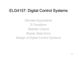
1. ELG4157: Digital Control Systems
Discrete Equivalents
Z-Transform
Stability Criteria
Steady State Error
Design of Digital Control Systems
1

2. Advantages and Disadvantages
• Improved sensitivity.
• Use digital components.
• Control algorithms easily
modified.
• Many systems inherently
are digital.
• Develop complex math
algorithms.
• Lose information during
conversions due to
technical problems.
• Most signals continuous
in nature.

3. Digitization
• The difference between the continuous and digital systems is that
the digital system operates on samples of the sensed plant rather
than the continuous signal and that the control provided by the
digital controller D(s) must be generated by algebraic equations.
• In this regard, we will consider the action of the analog-to-digital
(A/D) converter on the signal. This device samples a physical signal,
mostly voltage, and convert it to binary number that usually consists
of 10 to 16 bits.
• Conversion from the analog signal y(t) to the samples y(kt), occurs
repeatedly at instants of time T seconds apart.
• A system having both discrete and continuous signals is called
sampled data system.
• The sample rate required depends on the closed-loop bandwidth of
the system. Generally, sample rates should be about 20 times the
bandwidth or faster in order to assure that the digital controller will
match the performance of the continuous controller.
3

4. 4
Digital Control System
ADC
Micro
Processor
DAC
Correction
Element
Process
Clock
Measurement
+
-
A D D A
A: Analog
D: Digital

5. 5
Continuous Controller and Digital Control
Gc(s) Plant
R(t) y(t)
Continuous Controller
+
-
A/D Digital
Controller
D/A and
Hold
Plant
D/A
+
-
r(t)
Digital Controller
y(t)
r(kT) p(t)
m(t)
m(kT)

6. 6
Applications of Automatic Computer
Controlled Systems
• Most control systems today use digital computers
(usually microprocessors) to implement the controllers).
Some applications are:
• Machine Tools
• Metal Working Processes
• Chemical Processes
• Aircraft Control
• Automobile Traffic Control
• Automobile Air-Fuel Ratio
• Digital Control Improves Sensitivity to Signal Noise.

7. 7
Digital Control System
• Analog electronics can integrate and differentiate signals. In order
for a digital computer to accomplish these tasks, the differential
equations describing compensation must be approximated by
reducing them to algebraic equations involving addition, division,
and multiplication.
• A digital computer may serve as a compensator or controller in a
feedback control system. Since the computer receives data only at
specific intervals, it is necessary to develop a method for describing
and analyzing the performance of computer control systems.
• The computer system uses data sampled at prescribed intervals,
resulting in a series of signals. These time series, called sampled
data, can be transformed to the s-domain, and then to the z-domain
by the relation z = ezt.
• Assume that all numbers that enter or leave the computer has the
same fixed period T, called the sampling period.
• A sampler is basically a switch that closes every T seconds for one
instant of time.

8. 8
r(t) r*(t)
Continuous Sampled
Sampler
r(T)
r(2T)
r(3T)
r(kT)
r(4T)
0 T 2T 3T
T 2T 3T
4T
4T
Zero-order
Hold
Go(s)
P(t)
 
s
e
e
s
s
s
G
sT
sT

 



1
1
1
)
(
0

9. D/A
A/D Computer Process
Measure
r(t) c(t)
e(t)
－
e*(t) u*(t) u(t)
Sampling analysis
Expression of the sampling signal
Modeling of Digital Computer
)
(
)
(
)
(
)
(
)
(
)
(
)
(
*
0
0
kT
t
kT
x
kT
t
t
x
t
t
x
t
x
k
k
T 





 









10. 10
Analog to Digital Conversion: Sampling
An input signal is converted from continuous-varying
physical value (e.g. pressure in air, or frequency or
wavelength of light), by some electro-mechanical device
into a continuously varying electrical signal. This signal has
a range of amplitude, and a range of frequencies that can
present. This continuously varying electrical signal may
then be converted to a sequence of digital values, called
samples, by some analog to digital conversion circuit.
• There are two factors which determine the accuracy with which the
digital sequence of values captures the original continuous signal: the
maximum rate at which we sample, and the number of bits used in
each sample. This latter value is known as the quantization level

11. 11
Zero-Order Hold
• The Zero-Order Hold block samples and holds its input
for the specified sample period.
• The block accepts one input and generates one output,
both of which can be scalar or vector. If the input is a
vector, all elements of the vector are held for the same
sample period.
• This device provides a mechanism for discretizing one or
more signals in time, or resampling the signal at a
different rate.
• The sample rate of the Zero-Order Hold must be set to
that of the slower block. For slow-to-fast transitions, use
the unit delay block.

12. 12
The z-Transform
The z-Transform is used to take discrete time domain signals into a complex-
variable frequency domain. It plays a similar role to the one the Laplace
transform does in the continuous time domain. The z-transform opens up new
ways of solving problems and designing discrete domain applications. The z-
transform converts a discrete time domain signal, which is a sequence of real
numbers, into a complex frequency domain representation.













 












0
0
0
0
)
(
)
(
)}
(
{
1
)
(
)
(
)}
(
*
{
)}
(
{
)
(
)}
(
*
{
have
we
s,
transform
Laplace
the
Using
0,
signal
a
For
)
(
)
(
)
(
*
k
k
k
k
sT
k
ksT
k
z
kT
f
z
F
t
f
Z
z
z
z
U
z
kT
r
t
r
Z
t
r
Z
e
z
e
kT
r
t
r
t
kT
t
kT
r
t
r 

13. 13
Transfer Function of Open-Loop System
Zero-order
Hold Go(s)
Process
r(t) T=1 r*(t)
 
3678
.
0
3678
.
1
2644
.
0
3678
.
0
)
(
)
1
1
1
1
(
1
)
(
:
fraction
partial
into
Expanding
)
1
(
1
)
(
)
(
)
(
)
(
*
)
(
)
1
(
1
)
(
;
)
1
(
)
(
2
2
2





















z
z
z
z
G
s
s
s
e
s
G
s
s
e
s
G
s
G
s
G
s
R
s
Y
s
s
s
G
s
e
s
G
st
st
p
o
p
st
o

14. 14

15. 





















n
i
T
a
i
n
n
n
i
e
z
z
K
z
X
Then
a
s
K
a
s
K
a
s
K
a
s
a
s
a
s
A(s)
X(s)
If
1
2
2
1
1
2
1
)
(
:
)
(
)
)(
(
:
Example: T
T
e
z
z
e
z
z
z
z
s
s
s
Z
s
s
s
s
Z 2
5
15
1
10
2
5
1
15
10
)
2
)(
1
(
)
4
(
5




























Z-Transform
Z-transform method: Partial-fraction expansion approaches
Inverse Z-transform method: Partial-fraction expansion approaches
























n
i
kT
a
i
T
a
T
a
T
a
T
a
T
a
i
n
e
K
kT
X
then
e
s
z
K
e
z
z
K
e
s
e
z
e
z
A(z)
X(z)
If
1
2
1
)
(
:
)
(
)
)(
(
:
2
1
2
1
Example:
kT
T
T
T
e
e
z
z
z
z
Z
e
z
z
e
z
Z
kT
x 2
2
1
2
2
1
1
1
)
)(
1
(
)
1
(
)
( 






























16. 16
Closed-Loop Feedback Sampled-Data Systems
G(z)
r(t) R(z) E(z) Y(z)
Y(z)
)
(
)
(
1
)
(
)
(
)
(
1
)
(
)
(
)
(
)
(
z
D
z
G
z
D
z
G
z
G
z
G
z
T
z
R
z
Y





G(z)
R(z) E(z) Y(z)
Y(z)
D(z)

17. 17
Now Let us Continue with the Closed-Loop System for the
Same Problem
5
4
3
2
1
2
3
2
2
2
147
.
1
4
.
1
4
.
1
3678
.
0
)
(
6322
.
0
6322
.
1
2
2644
.
0
3678
.
0
)
6322
.
0
)(
1
(
)
2644
.
0
3678
.
0
(
)
(
1
)
(
:
input
step
unit
a
an
Assume
6322
.
0
2644
.
0
3678
.
0
)
(
1
)
(
)
(
)
(




























z
z
z
z
z
z
Y
z
z
z
z
z
z
z
z
z
z
z
Y
z
z
z
R
z
z
z
z
G
z
G
z
R
z
Y

18. Stability
• The difference between the stability of the continuous
system and digital system is the effect of sampling rate
on the transient response.
• Changes in sampling rate not only change the nature of
the response from overdamped to underdamped, but
also can turn the system to an unstable.
• Stability of a digital system can be discussed from two
perspectives:
• z-plane
• s-plane
18

19. 19
Stability Analysis in the z-Plane
A linear continuous feedback control system is stable if all poles of the
closed-loop transfer function T(s) lie in the left half of the s-plane.
In the left-hand s-plane,   0; therefore, the related magnitude of z
varies between 0 and 1. Accordingly the imaginary axis of the s-plane
corresponds to the unit circle in the z-plane, and the inside of the unit
circle corresponds to the left half of the s-plane.
A sampled system is stable if all the poles of the closed-loop transfer
function T(z) lie within the unit circle of the z-plane.
T
z
e
z
e
e
z
T
T
j
sT








  )
(

20. 1 Re
Im
z-plane
Stable zone
The graphic expression of the stability
condition for the sampling control systems
The stability criterion
In the characteristic equation 1+GH(z)=0, substitute z with
1
1



s
s
z —— Bilinear transformation
We can analyze the stability of the sampling control systems the same as we did
in chapter 3 (Routh criterion in the s-plane) .






























































)
(
)
(
1
0
1
0
)
1
(
2
)
1
(
1
1
1
1
1
1
1
:
,
,
:
2
2
2
2
2
2
2
2
2
2
z-plane
le of the
unit circ
inside the
e
the s-plan
of
ft half
for the le
y
x
y
x
y
x
y
j
y
x
y
x
jy
x
jy
x
jy
x
jy
x
z
z
j
s
then
jy
x
z
j
w
suppose
Proof





The Stability Analysis
Unstable zone
Critical stability

21. 0
368
.
0
368
.
1
632
.
0
1
)
(
1 2






z
z
Kz
z
G
Determine K for the stable system
Solution:
0
)
632
.
0
736
.
2
(
264
.
1
632
0
0
368
.
0
368
.
1
632
.
0
1 2








 K
s
Ks
.
z
z
Kz
K
K
K
.
n
h criterio
f the Rout
In terms o
632
.
0
736
.
2
264
.
1
632
.
0
736
.
2
632
0
:


We have: 0 < K < 4.33
1
1



s
s
z
Make
The Stability Analysis

22. 22
Example: Stability of a closed-loop system
Gp(s)
r(t) Y(t)
Go(s)
gain.
of
values
all
for
stable
is
continuous
the
gain where
increased
for
unstable
is
system
sampled
order
-
Second
39
.
2
0
:
for
stable
is
system
This
unstable)
(
)
295
.
1
115
.
1
(
)
295
.
1
115
.
1
(
012
.
3
310
.
2
2
10
When
circle,
unit
e
within th
lie
roots
the
because
stable
is
system
The
0
)
6182
.
0
5
.
0
)(
6182
.
0
5
.
0
(
6322
.
0
2
;
1
0
)
1
(
2
:
0
G(z)]
[1
equation
the
of
roots
the
are
(z)
function t
transfer
loop
-
losed
the
of
poles
The
)
1
(
2
)
(
3678
.
0
3678
.
1
2
)
2644
.
0
3678
.
0
(
)
(
;
)
1
(
)
(






































K
j
z
j
z
z
z
K
j
z
j
z
z
z
K
Kb
Kaz
a
z
a
z
a
z
a
z
b
az
K
z
z
z
K
z
G
s
s
K
s
p
G

23. Example
23

25. The Steady State Error Analysis
)
(
1
)
(
)
(
1
)
(
)
(
)
(
)
(
)
(
)
(
z
G
z
R
z
G
z
G
z
R
z
R
z
c
z
R
z
E







G(s)
r c
－
e




















*
2
*
*
1
1
1
1
)
(
1
)
(
)
1
(
lim
)
(
)
1
(
lim
a
v
p
z
z
ss
K
T
K
T
K
z
G
z
R
z
z
E
z
e
)
(
)
1
(
lim
;
)
1
(
)
1
(
)
(
)
(
)
(
)
1
(
lim
;
)
1
(
)
(
)
(
)
(
lim
;
1
)
(
)
(
1
)
(
2
1
*
3
2
2
1
*
2
1
*
z
G
z
K
z
z
z
T
z
R
t
t
r
z
G
z
K
z
Tz
z
R
t
t
r
z
G
K
z
z
z
R
t
t
r
z
a
z
v
z
p





















)
(
)
1
(
lim
1
z
E
z
e
z
ss 



26. )
5
(
)
(
1



s
s
K
s
G
s
T
2) If r(t) = 1+t, determine ess=？
1) Determine K for the stable system.
Solution








































5
25
5
5
)
1
(
)
5
(
)
1
(
)
5
(
1
)
(
2
2
s
K
s
K
s
K
Z
e
s
s
K
Z
e
s
s
K
s
e
Z
z
G
Ts
Ts
Ts
1)
)
0067
.
0
)(
1
(
2135
.
0
2067
.
2
5
25
1
5
)
1
(
5
)
1
(
2
1
5
2
1



























z
z
z
z
K
e
z
Kz
z
Kz
z
KTz
z
T
T
r
－ G (s)
c
Z.O.H
e
Example

27. 0
)
4202
.
2
067
.
10
(
)
1.573
9.993
(
0.9932
1
1
0
)
2135
.
0
0335
.
0
(
)
0335
.
5
2067
.
2
(
)
5
(
0
)
0067
.
0
)(
1
(
2135
.
0
2067
.
2
5
1
)
(
1
:
system
the
of
equation
stic
charecteri
The
2
2























K
w
K
w
s
s
z
K
z
K
z
-K
z
z
z
z
K
z
G
16
.
4
0 
 K
2)
K
K
T
K
T
K
e
K
z
z
z
K
z
G
z
K
z
z
z
z
K
z
G
K
v
p
ss
z
z
v
z
z
p
5
2
.
0
0
1
1
2
.
0
)
0067
.
0
(
2135
.
0
2067
.
2
5
lim
)
(
)
1
(
lim
)
0067
.
0
)(
1
(
2135
.
0
2067
.
2
5
lim
)
(
lim
1
T
*
*
2
1
1
*
2
1
1
*






























28. Steady State Error and System Type

29. 1) For unity feedback in figure below,
2)

30. 30
Design of Digital Control Systems
The Procedure:
• Start with continuous system.
• Add sampled-data system elements.
• Chose sample period, usually small but not too small.
Use sampling period T = 1 / 10 fB, where fB = B / 2 and
B is the bandwidth of the closed-loop system.
– Practical limit for sampling frequency: 20 ˂ s / B ˃40
• Digitize control law.
• Check performance using discrete model or SIMULINK.

31. 31

32. 32
Start with a Continuous Design
D(s) may be given as an existing design or by using root
locus or bode design.
G(z)
r(t) R(z)
E(z)
Y(z)
Y(z)
D(z)

33. 33
Add Samples Necessary for Digital Control
• Transform D(s) to D(z): We will obtain a discrete system
with a similar behavior to the continuous one.
• Include D/A converter, usually a zero-order-device.
• Include A/D converter modeled as an ideal sampler.
• And an antialiasing filter, a low pass filter, unity gain filter
with a sharp cutoff frequency.
• Chose a sample frequency based on the closed-loop
bandwidth B of the continuous system.

34. 34
Closed-Loop System with Digital Computer Compensation
 
  
 
 
 
  
 
  b
a
K
B
A
C
e
B
e
A
z
D
s
G
Z
B
z
A
z
C
z
D
b
s
a
s
K
s
G
z
z
z
z
D
z
G
z
z
z
D
K
r
z
z
G
r
z
z
k
z
D
z
z
z
G
T
s
s
s
Gp
z
D
z
E
z
U
z
D
z
G
z
D
z
G
z
T
z
R
z
Y
bT
aT
c
c 



































1
1
;
;
);
(
)}
(
{
;
)
(
;
)
(
240
.
0
1
7189
.
0
5
.
0
)
(
)
(
;
240
.
0
7189
.
0
359
.
1
)
(
.
and
parameters
two
the
have
and
3678
.
0
at
)
(
of
pole
cancer the
We
)
(
)
3678
.
0
(
)
(
select
we
If
;
3678
.
0
1
0.7189
z
0.3678
)
(
1;
when
)
1
(
1
)
(
plant
a
and
hold
order
-
zero
a
with
system
order
second
he
Consider t
)
(
)
(
)
(
is
computer
the
of
function
tranfer
The
)
(
)
(
1
)
(
)
(
)
(
)
(
)
(

35. 35
Compensation Networks (10.3; page 747)
The compensation network, Gc(s) is cascaded with the unalterable process
G(s) in order to provide a suitable loop transfer function Gc(s)G(s)H(s).
G(s)
R(s)
Gc(s)
+
-
H(s)
Y(s)
Compensation
 
network
lead
-
phase
a
called
is
network
the
p,
z
When
r
compensato
order
First
)
(
)
(
)
(
)
(
)
(
)
(
1
1





 
 



p
s
z
s
K
s
G
p
s
z
s
K
s
G
c
N
j
i
M
i
i
c
j

-z
-p

36. 36
Closed-Loop System with Digital Computer Compensation
There are two methods of compensator design:
(1) Gc(s)-to-D(z) conversion method, and
(2) Root locus z-plane method.
The Gc(s)-to-D(z) Conversion Method
 
 
0
when
1
1
;
;
transform)
-
(z
)
(
)}
(
{
)
Controller
(Digital
)
(
r)
Compensato
Order
-
(First
)
(















s
b
a
K
B
A
C
e
B
e
A
z
D
s
G
Z
B
z
A
z
C
z
D
b
s
a
s
K
s
G
bT
aT
c
c

37. The Frequency Response
The frequency response of a system is defined as the
steady-state response of the system to a sinusoidal input
signal.
The sinusoid is a unique input signal, and the resulting
output signal for a linear system, as well as signals
throughout the system, is sinusoidal in the steady-state; it
differs form the input waveform only in amplitude and
phase.
37

38. Phase-Lead Compensator Using Frequency Response
A first-order phase-lead compensator can be designed using the frequency
response. A lead compensator in frequency response form is given by
In frequency response design, the phase-lead compensator adds positive phase to
the system over the frequency range. A bode plot of a phase-lead compensator
looks like the following
Gc s
( )
1  
 s


 
 1  s


 

p
1

z
1

m z p
 sin m
   1

 1


39. Phase-Lead Compensator Using Frequency Response
Additional positive phase increases the phase margin and
thus increases the stability of the system. This type of
compensator is designed by determining alfa from the
amount of phase needed to satisfy the phase margin
requirements.
Another effect of the lead compensator can be seen in the
magnitude plot. The lead compensator increases the gain of
the system at high frequencies (the amount of this gain is
equal to alfa. This can increase the crossover frequency,
which will help to decrease the rise time and settling time of
the system.

40. Phase-Lag Compensator Using Root Locus
A first-order lag compensator can be designed using the root locus. A lag
compensator in root locus form is given by
where the magnitude of z is greater than the magnitude of p. A phase-lag
compensator tends to shift the root locus to the right, which is undesirable. For this
reason, the pole and zero of a lag compensator must be placed close together
(usually near the origin) so they do not appreciably change the transient response
or stability characteristics of the system.
When a lag compensator is added to a system, the value of this intersection will be
a smaller negative number than it was before. The net number of zeros and poles
will be the same (one zero and one pole are added), but the added pole is a
smaller negative number than the added zero. Thus, the result of a lag
compensator is that the asymptotes' intersection is moved closer to the right half
plane, and the entire root locus will be shifted to the right.
Gc s
( )
s z

( )
s p

( )

41. Lag or Phase-Lag Compensator using Frequency Response
A first-order phase-lag compensator can be designed using the frequency
response. A lag compensator in frequency response form is given by
The phase-lag compensator looks similar to a phase-lead compensator, except
that a is now less than 1. The main difference is that the lag compensator adds
negative phase to the system over the specified frequency range, while a lead
compensator adds positive phase over the specified frequency. A bode plot of a
phase-lag compensator looks like the following
Gc s
( )
1  
 s


 
 1  s


 


42. 42
Example: Design to meet a Phase Margin Specification
Based on Chapter 10 (Dorf): Example 13.7
 
differ!
would
)
(
of
t
coefficien
the
the
period,
sampling
for the
lue
another va
select
we
If
)
73
.
0
(
)
95
.
0
(
85
.
4
)
(
4.85;
and
0.73,
e
,
95
.
0
have
We
second.
0.001
Set
).
(
by
realized
be
to
is
)
(
r
compensato
the
Now
5.6.
Then
rad/s.
125
When
1
)
(
yield
order to
in
select
We
)
312
(
)
50
(
)
(
;
312
and
;
50
;
10.18).
(Eq
6.25
is
ratio
zero
-
pole
required
that the
find
we
10.4,
on
Based
10.24).
(Eq
2
is
margin
phase
that the
find
we
),
(
of
diagram
Bode
the
Using
10.10).
(Fig
rad/s
125
frequeny
crossover
a
with
45
of
margin
phase
a
achieve
that we
so
)
(
design
attempt to
will
We
.
)
1
25
.
0
(
1740
)
(
0.312
-
05
.
0
2
1
o
c
o
z
D
z
z
z
D
C
B
e
A
T
z
D
s
G
K
jω
GG
K
s
s
K
s
G
b
a
ab
s
G
s
G
s
s
s
G
c
c
c
c
c
p
c
p






























43. 43
The Root Locus of Digital Control Systems
D(z)
Zero
Order
hold
KGp(s)
R(s)
+
-
Y(s)
o
k
o
z
D
z
KG
z
D
z
KG
z
D
z
KG
z
D
z
KG
z
D
z
KG
z
D
z
KG
z
R
z
Y
360
180
)
(
)
(
and
1
)
(
)
(
or
0
)
(
)
(
1
4.
axis.
real
horizontal
the
respect to
with
l
symmetrica
is
locus
root
The
3.
zeros.
and
poles
of
number
odd
an
of
left
the
to
axis
real
the
of
section
a
on
lies
locus
root
The
2.
zeros.
the
to
progresses
and
poles
at the
starts
locus
root
The
1.
K varies.
as
system
sampled
the
of
equation
stic
characteri
for the
locus
root
Plot the
equation)
istic
(Character
0
)
(
)
(
1
;
)
(
)
(
1
)
(
)
(
)
(
)
(











44. 44
Re {z}
Im {z}
2 poles at
z = 1
0
-1
One zero
At z = -1
-3 -2
Root locus
1
;
3
;
0
)
(
)
(
)
1
(
)
1
(
for
solve
and
Let
0
)
1
(
)
1
(
1
)
(
1
2
1
2
2
























d
dF
F
K
K
z
z
z
K
z
KG
Unit circle
K increasing
Unstable
System
Order
Second
a
of
Locus
Root

45. 45
Design of a Digital Controller
plane.
-
z
on the
circle
unit
in the
point with
desired
a
at
roots
complex
of
set
a
give
will
system
d
compensate
the
of
locus
that the
so
b)
-
(z
Select
plane.
-
z
the
of
axis
real
positive
on the
lies
that
G(z)
at
pole
one
cancel
to
a)
-
(z
Use
)
(
)
(
)
(
controller
a
select
will
we
method,
locus
root
a
utilizing
response
specified
a
achieve
order to
In
b
z
a
z
z
D




46. 46
Example: Design of a digital compensator
0.8.
K
for
stable
is
system
the
Thus
0.8.
at
circle
unit
on the
is
locus
root
The
-2.56.
z
as
point
entry
obtain the
we
),
(
for
equation
the
Using
)
2
.
0
)(
1
(
)
1
(
)
(
)
(
have
we
0.2,
and
1
select
we
If
)
(
)
1
(
)
)(
1
(
)
(
)
(
)
(
Select
system.
unstable
have
we
1,
)
(
With
13.8.
Example
in
described
as
is
)
(
when
system
stable
a
in
result
that will
D(z)
r
compensato
a
design
us
Let
2


















K
F
z
z
z
k
z
D
z
KG
b
a
b
z
z
a
z
z
K
z
D
z
KG
b
z
a
z
z
D
z
D
s
Gp


47. 47
origin.
at the
is
equation
stic
characteri
the
of
root
the
1,
K
When
plane.
-
the
of
axis
real
on the
lie
would
locus
root
Then the
)
1
(
)
98
.
0
)(
1
(
)
1
(
)
(
)
(
that
so
0.98
-
and
1
selecting
by
locus
root
the
improve
would
we
,
inadequate
were
e
performanc
system
the
If









z
z
K
z
z
z
K
z
D
z
KG
b
a

48. 48
+1
0.2
-1
Unit circle
K=0.8
Im{z}
Re{z}
K increasing
Entry point at
z = -2.56
Root locus

49. 49
P13.10 Dorf
0.55.
is
overshoot
The
.
6843
.
0
4641
.
0
are
poles
the
119.5,
n
Whe
(f)
5661
.
0
092
.
1
1982
.
0
2759
.
0
)
(
75;
When
(e)
75.
find
we
0.3,
of
overshoot
maximum
and
1
for
13.19
Figure
Using
(d)
239.
is
of
value
maximum
method,
locus
root
Using
(c)
0
3679
.
0
368
.
1
0026
.
0
0037
.
0
1
is
equation
stic
characteri
system
loop
-
closed
The
(b)
3679
.
0
368
.
1
0026
.
0
0037
.
0
)
(
)
(
function
transfer
The
(a)
)
(
;
1
.
0
;
)
10
(
1
)
(
2
2
2
j
z
K
z
z
z
z
T
K
K
T/τ
K
z
z
z
K
z
z
z
K
z
D
z
G
K
z
D
T
s
s
s
Gp
























50. 50
P13.11 Dorf
150
;
999
.
0
;
993
.
0
1
1
;
;
999
.
0
993
.
0
150
)
(
:
0.01)
(
method
)
(
to
)
(
Use
(d)
3
.
155
;
99
.
0
;
9324
.
0
1
1
;
;
99
.
0
9324
.
0
3
.
155
)
(
:
0.1)
(
method
)
(
to
)
(
Use
(b)
.
01
.
0
and
30%
are
input)
ramp
a
(for
error
tracking
state
-
safety
and
overshoot
system
d
compensate
The
150.
and
0.1,
0.7,
select
may
we
Plot,
Bode
using
By
)
(
(a)
01
.
0
07
.
0
01
.
0
007
.
0


















































C
e
B
e
A
b
a
K
B
A
C
e
B
e
A
z
z
B
z
A
z
C
z
D
T
z
D
s
G
C
e
B
e
A
b
a
K
B
A
C
e
B
e
A
z
z
B
z
A
z
C
z
D
T
z
D
s
G
e
PO
K
b
a
b
s
a
s
K
s
G
bT
aT
c
bT
aT
c
ss
c