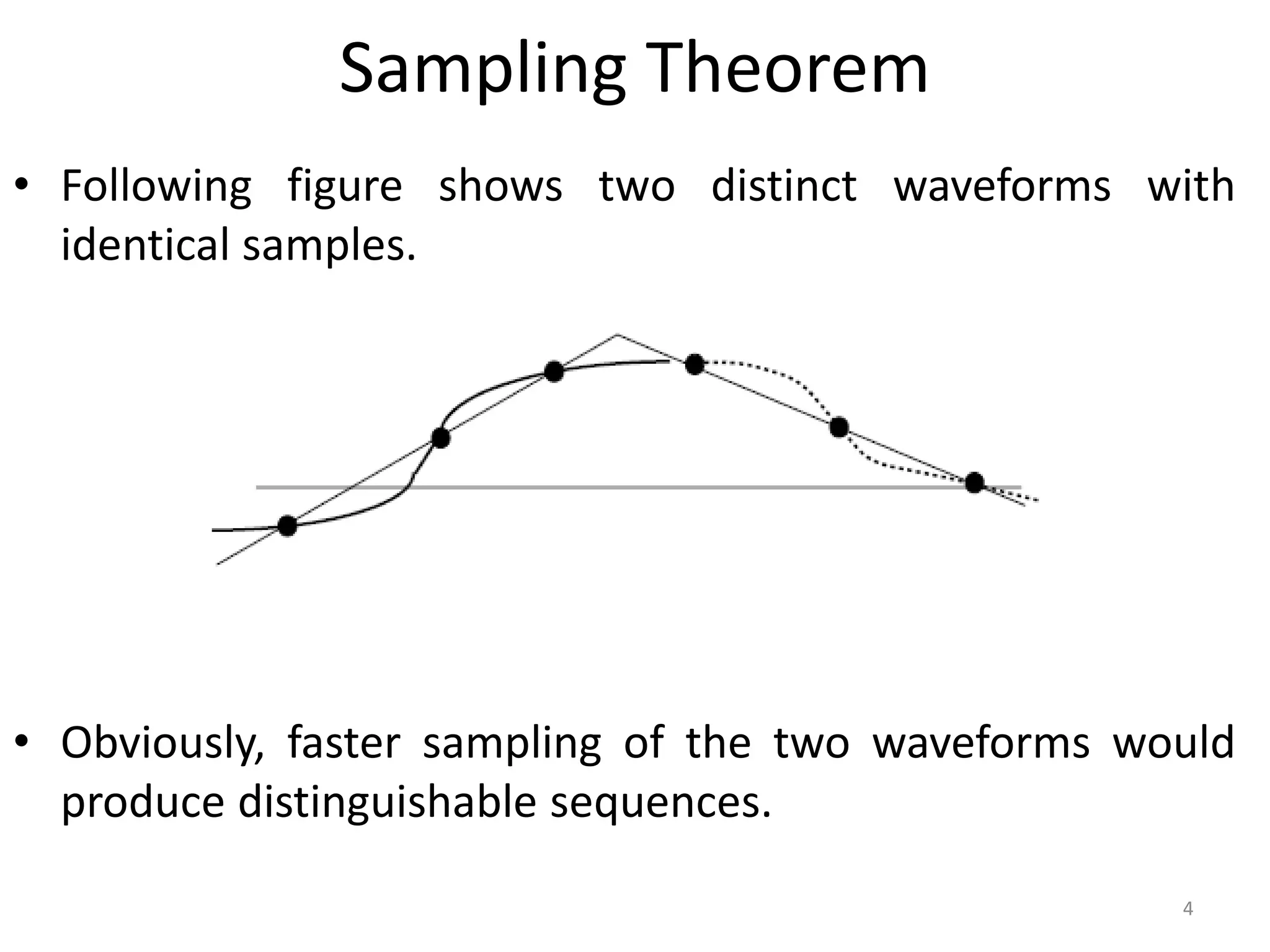
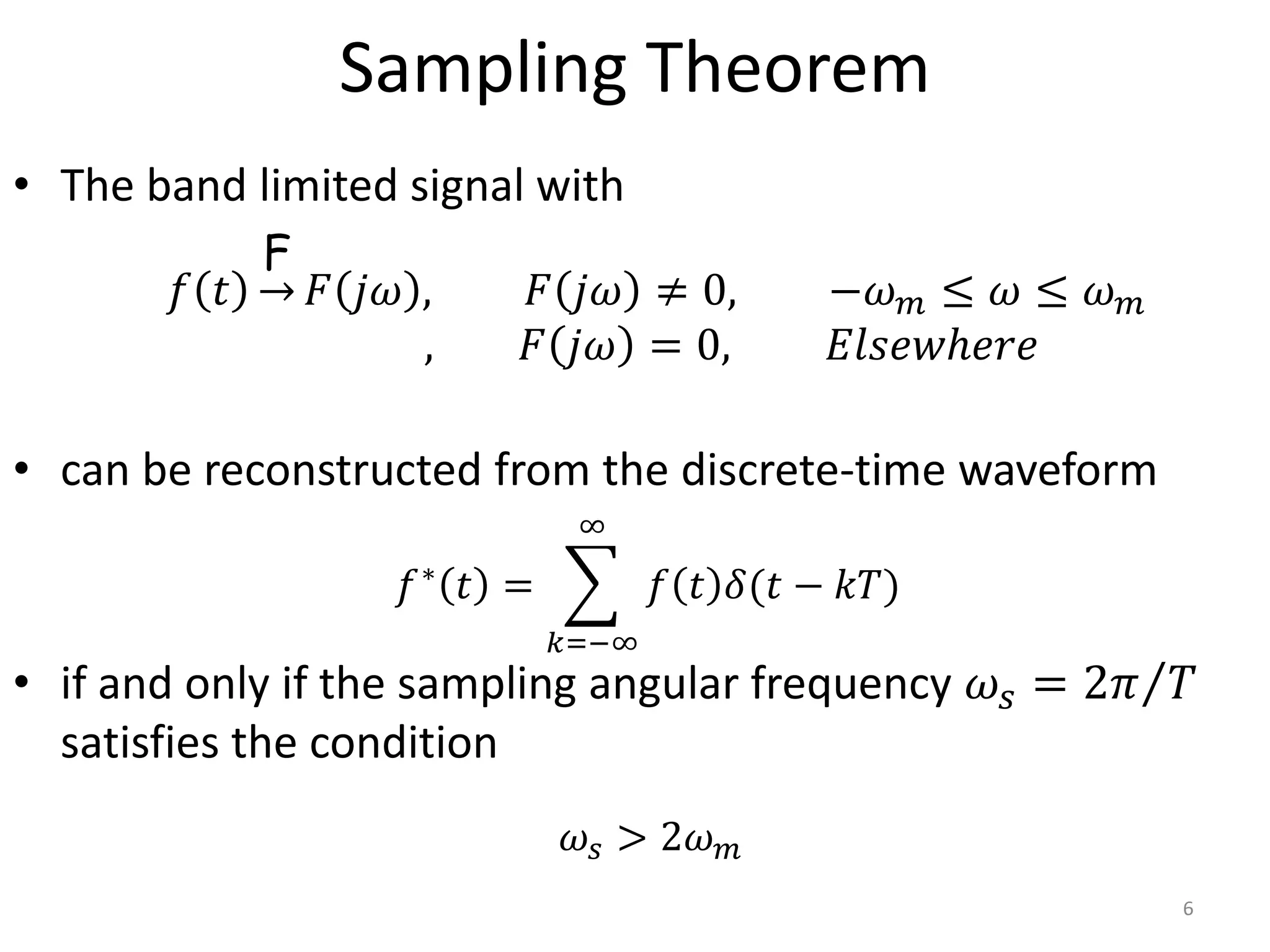
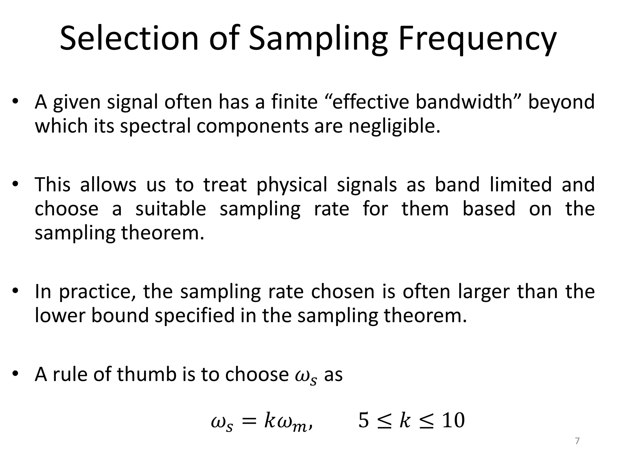
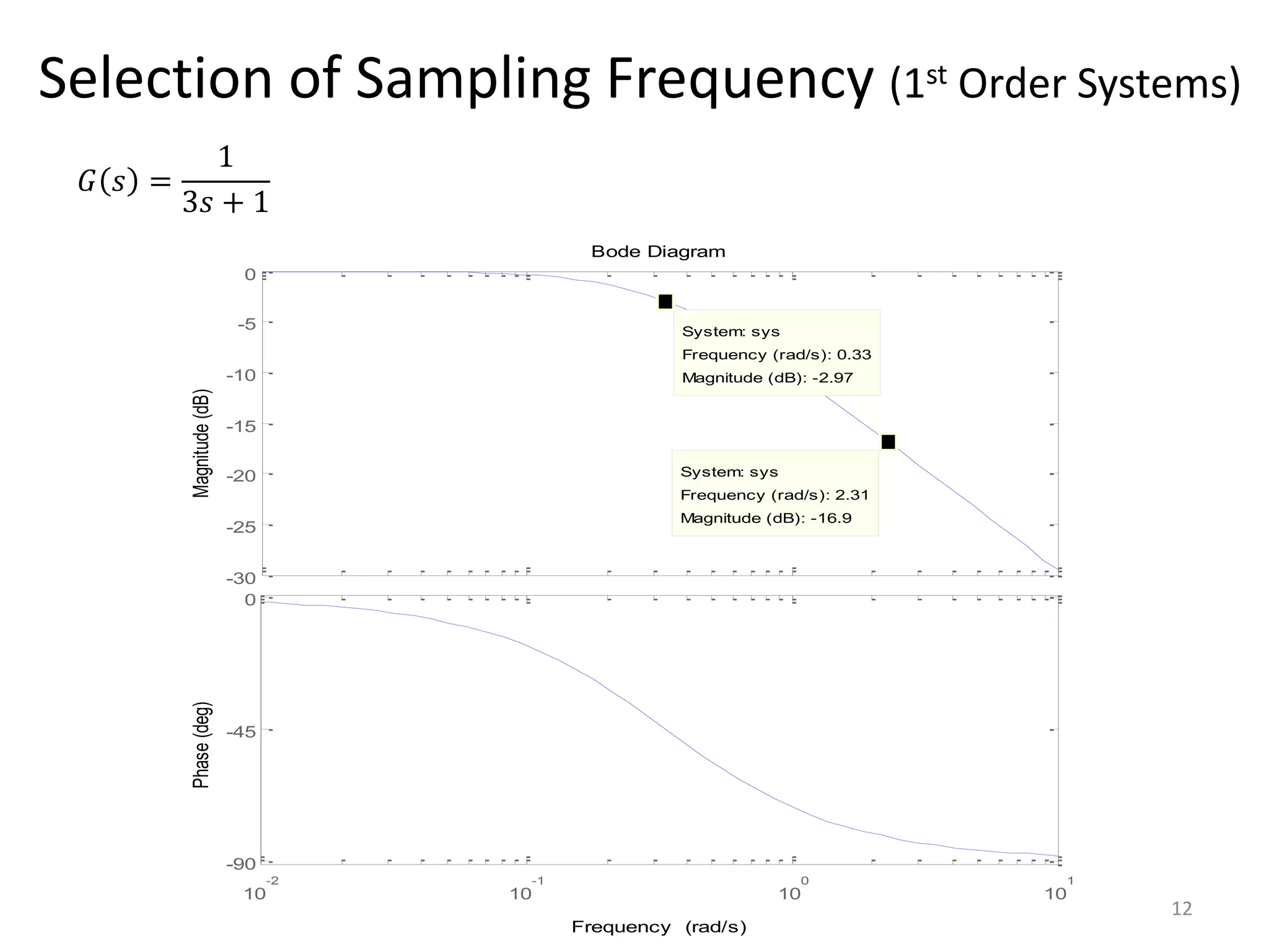
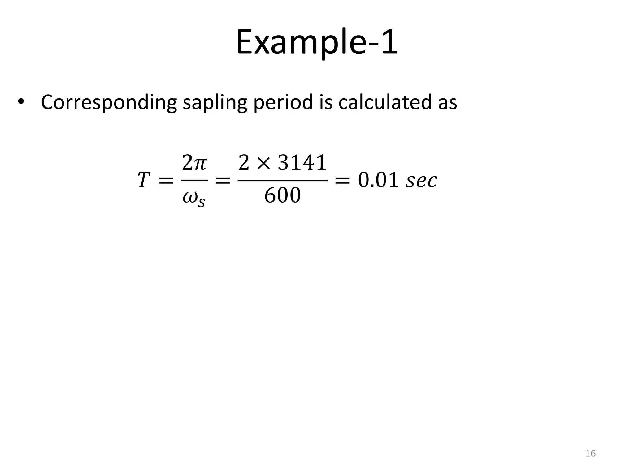
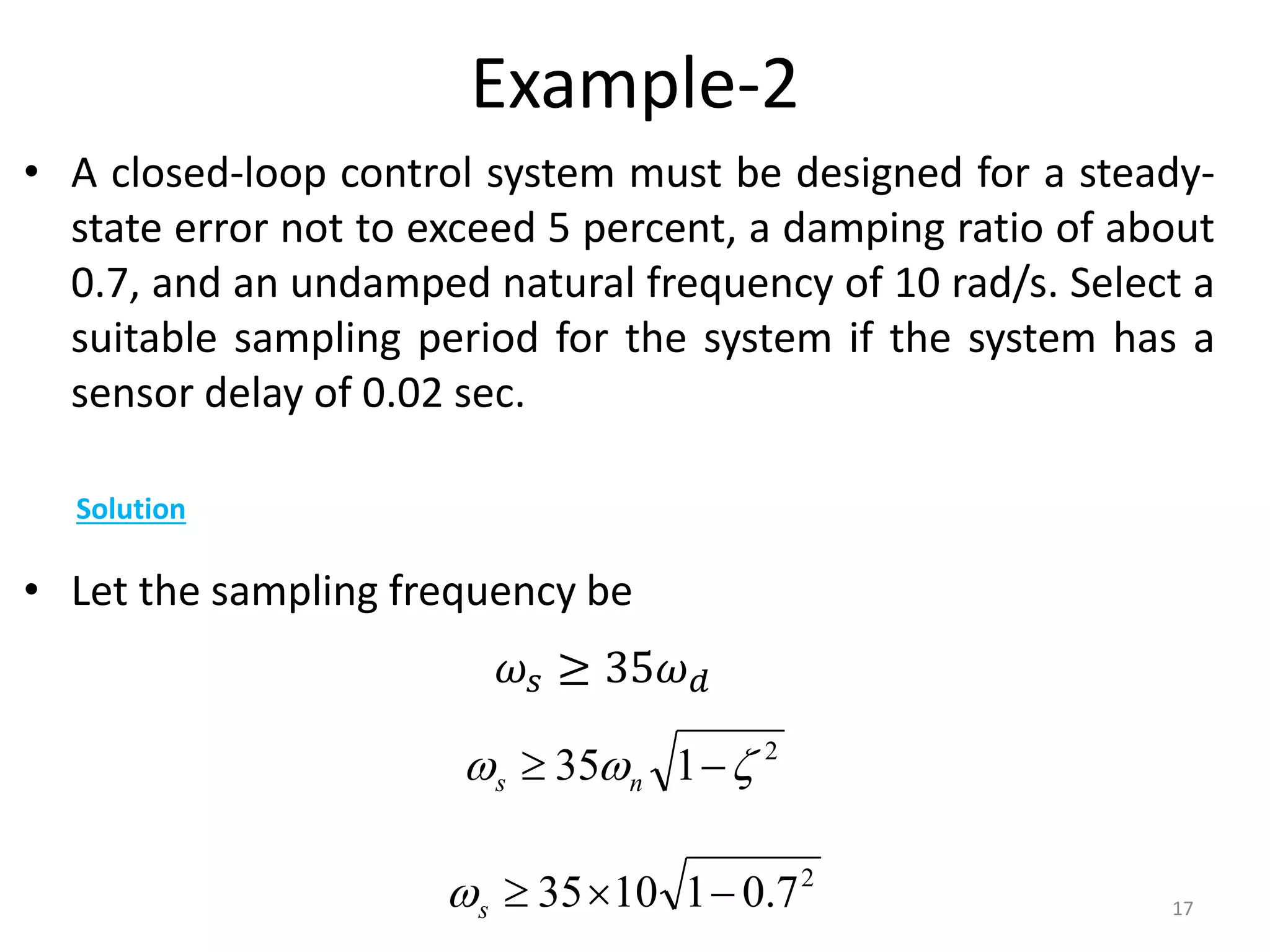
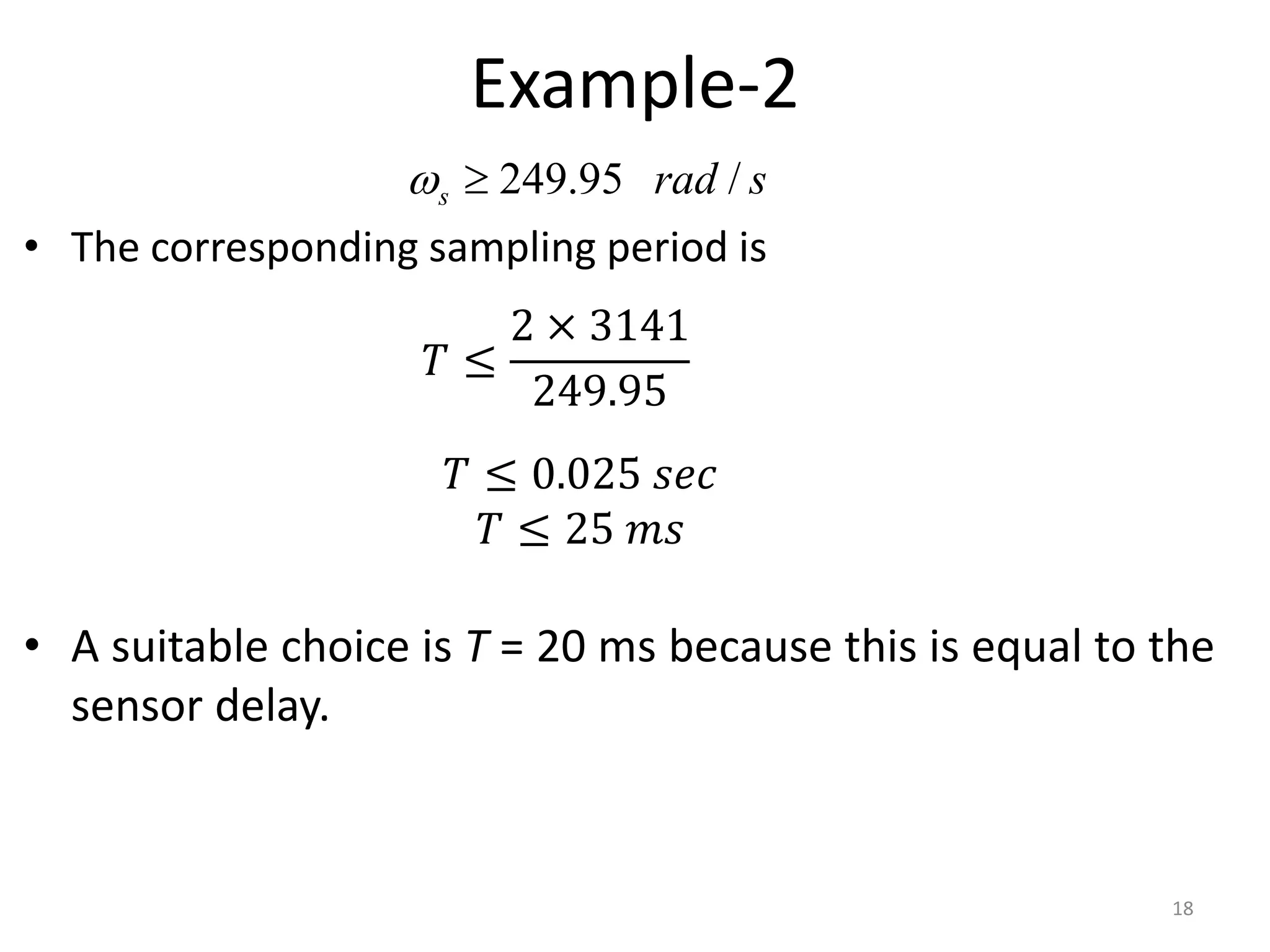
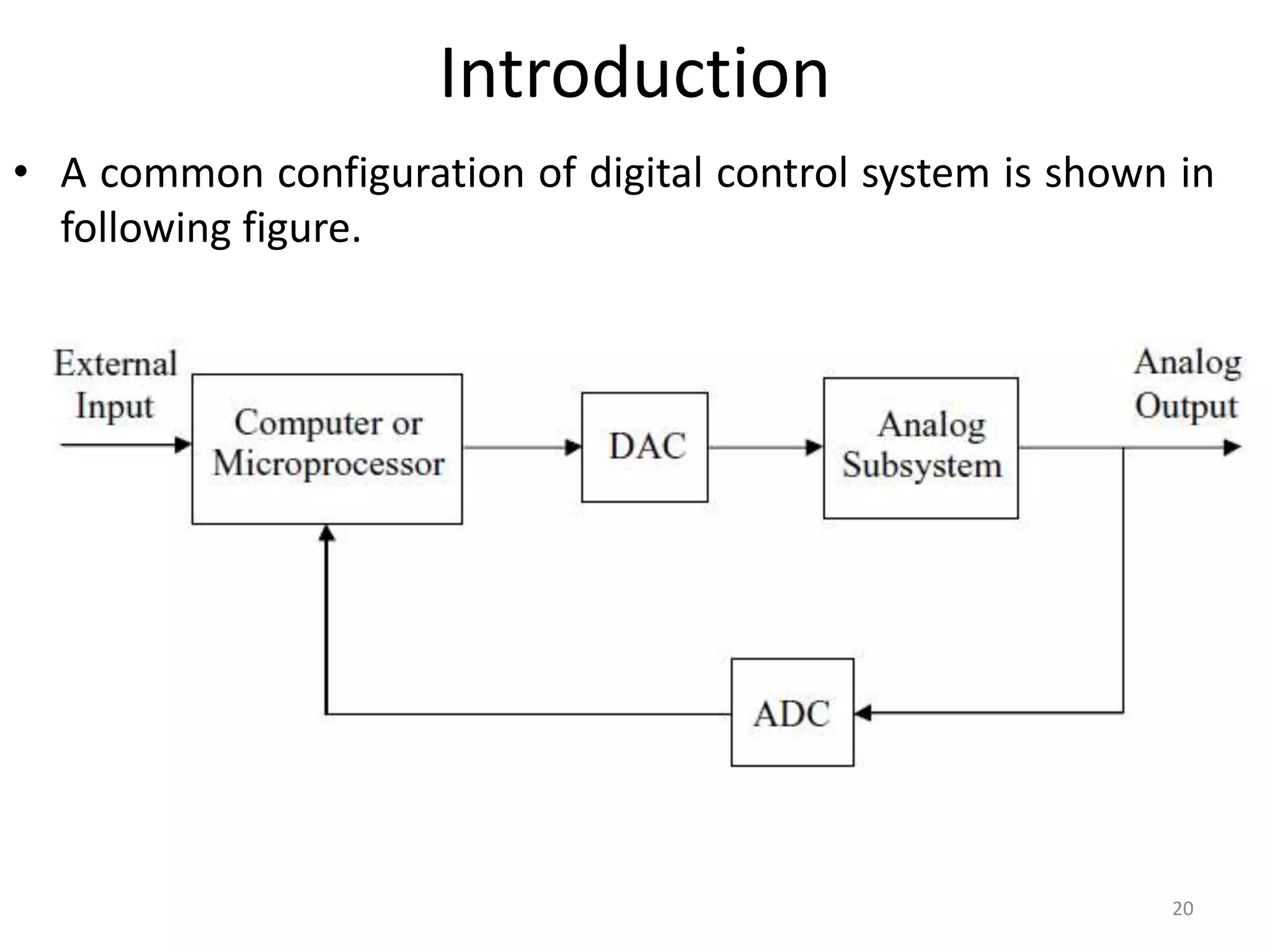
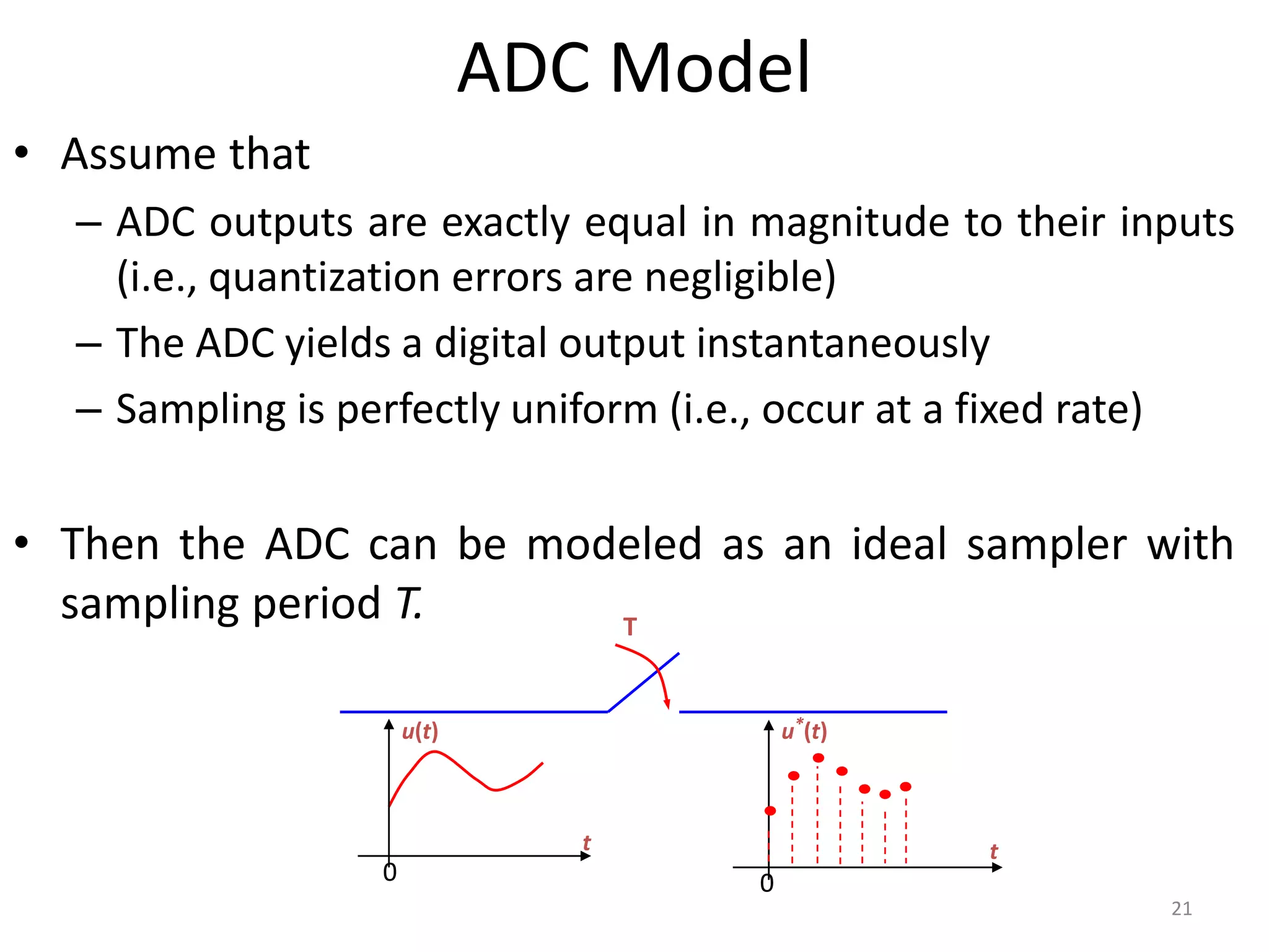
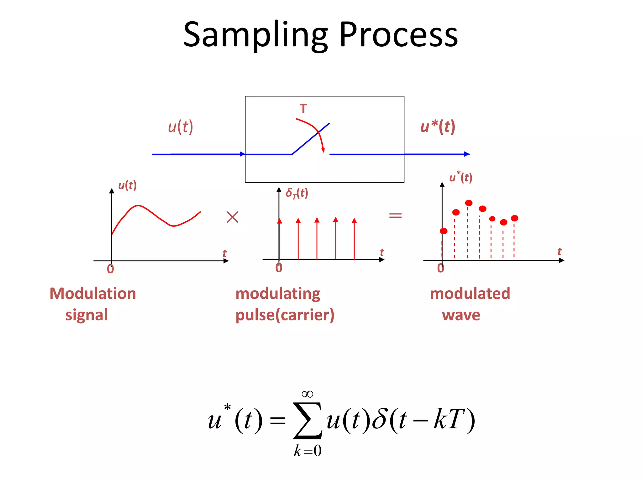
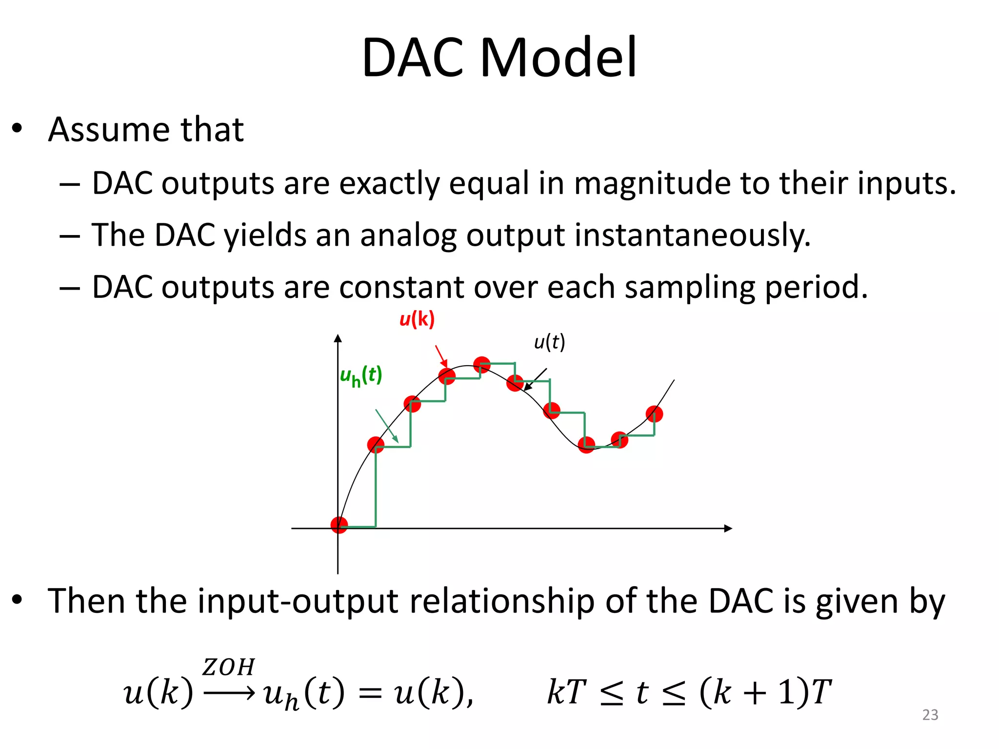
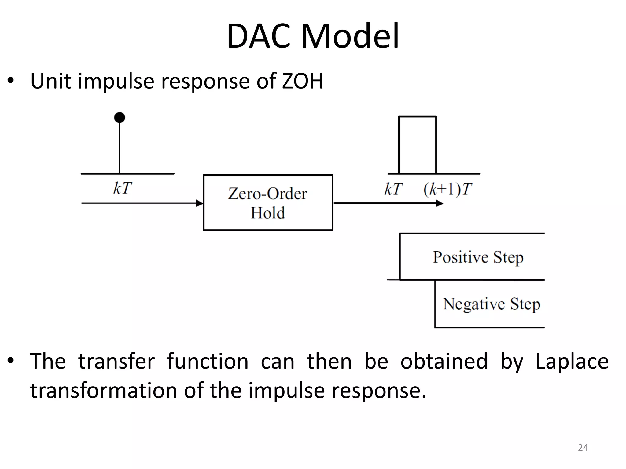
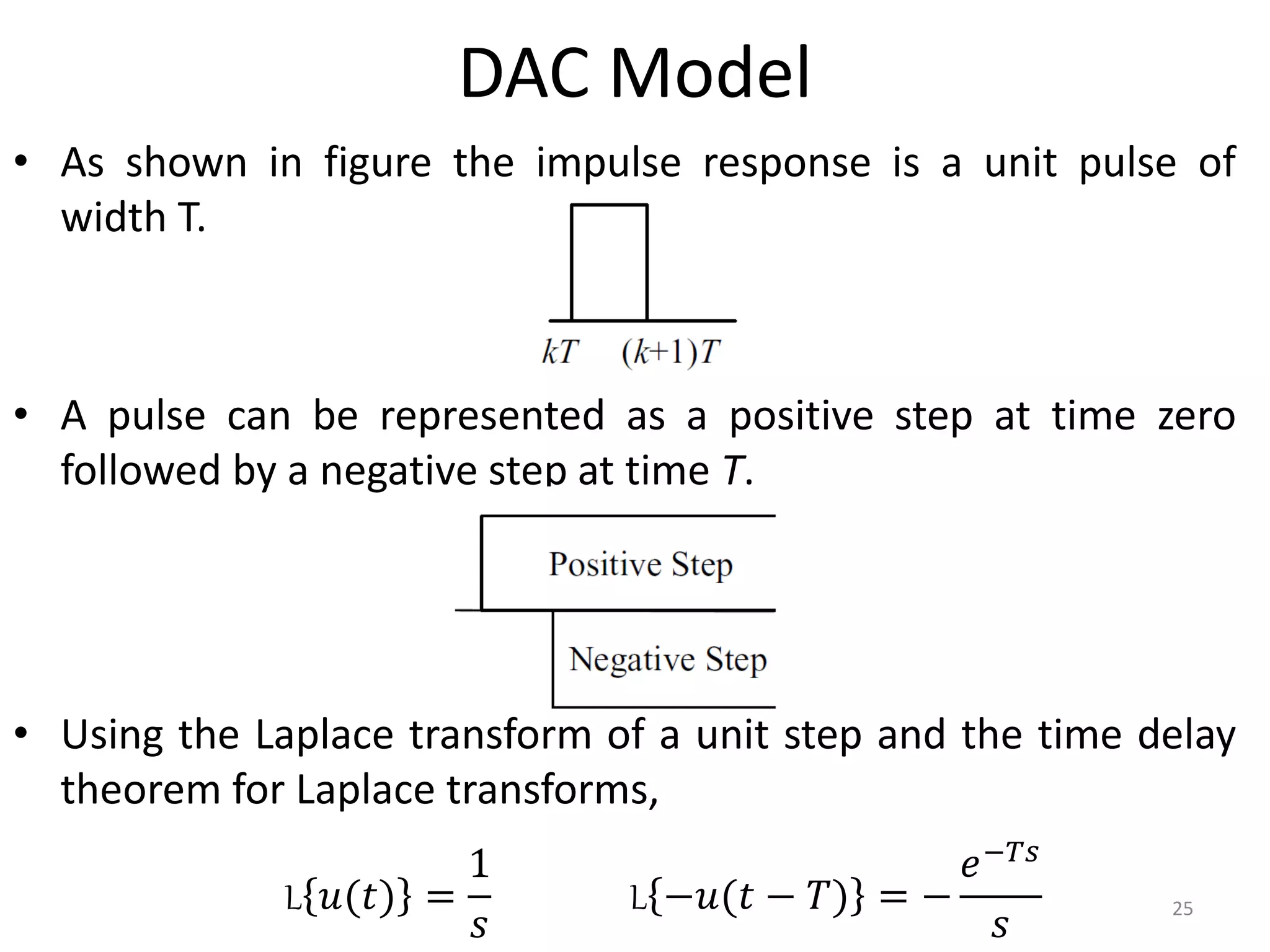
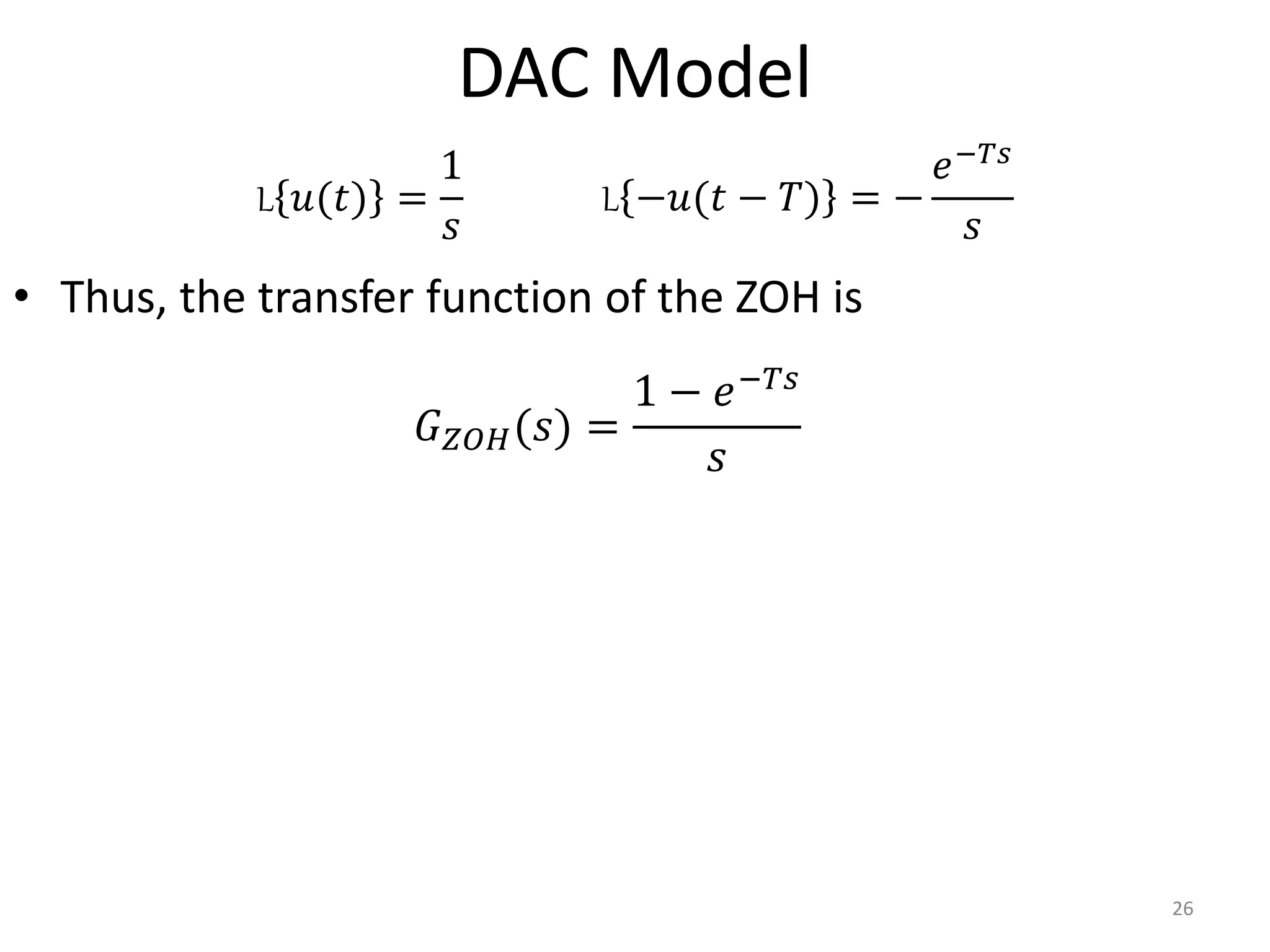
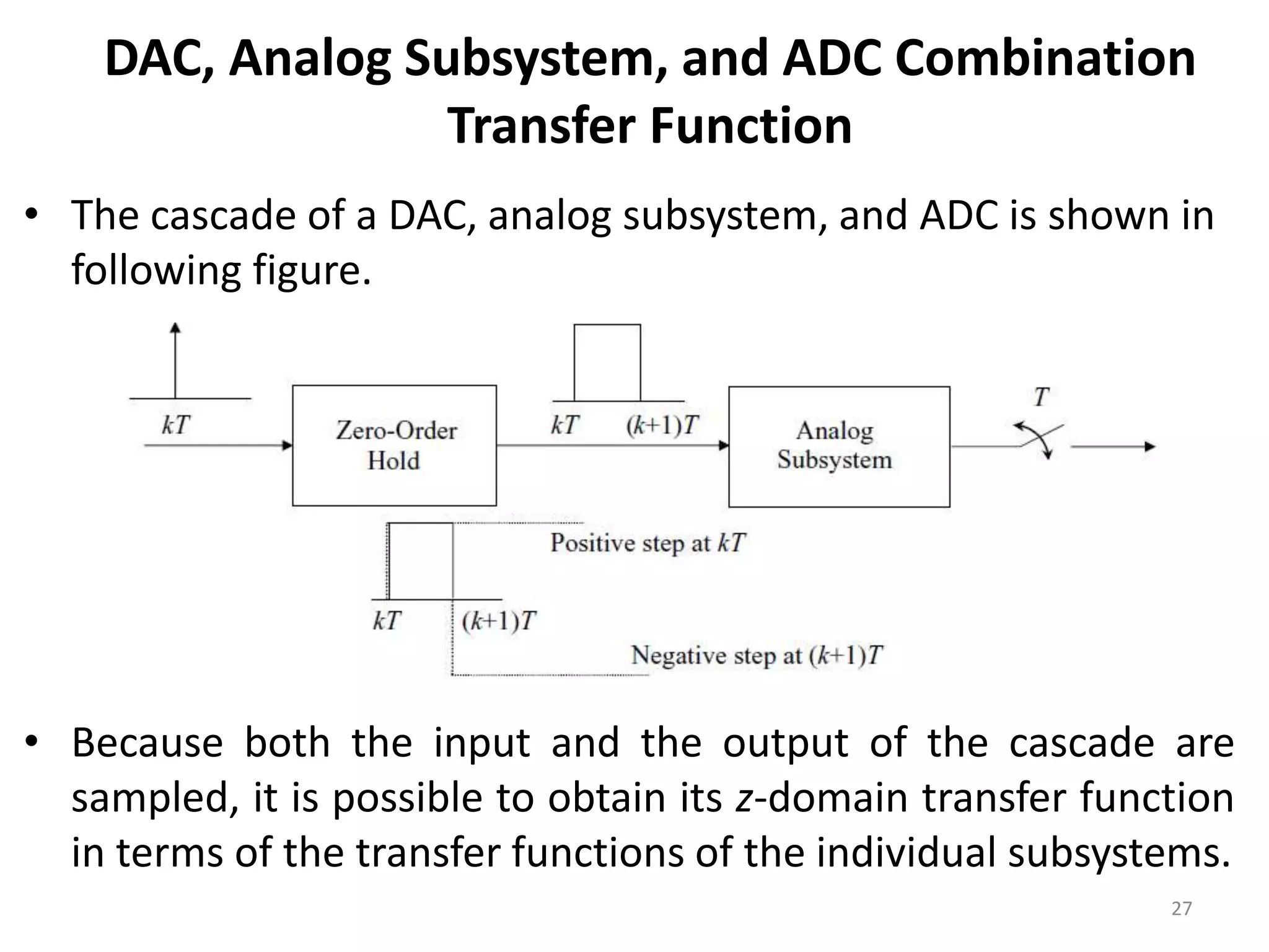
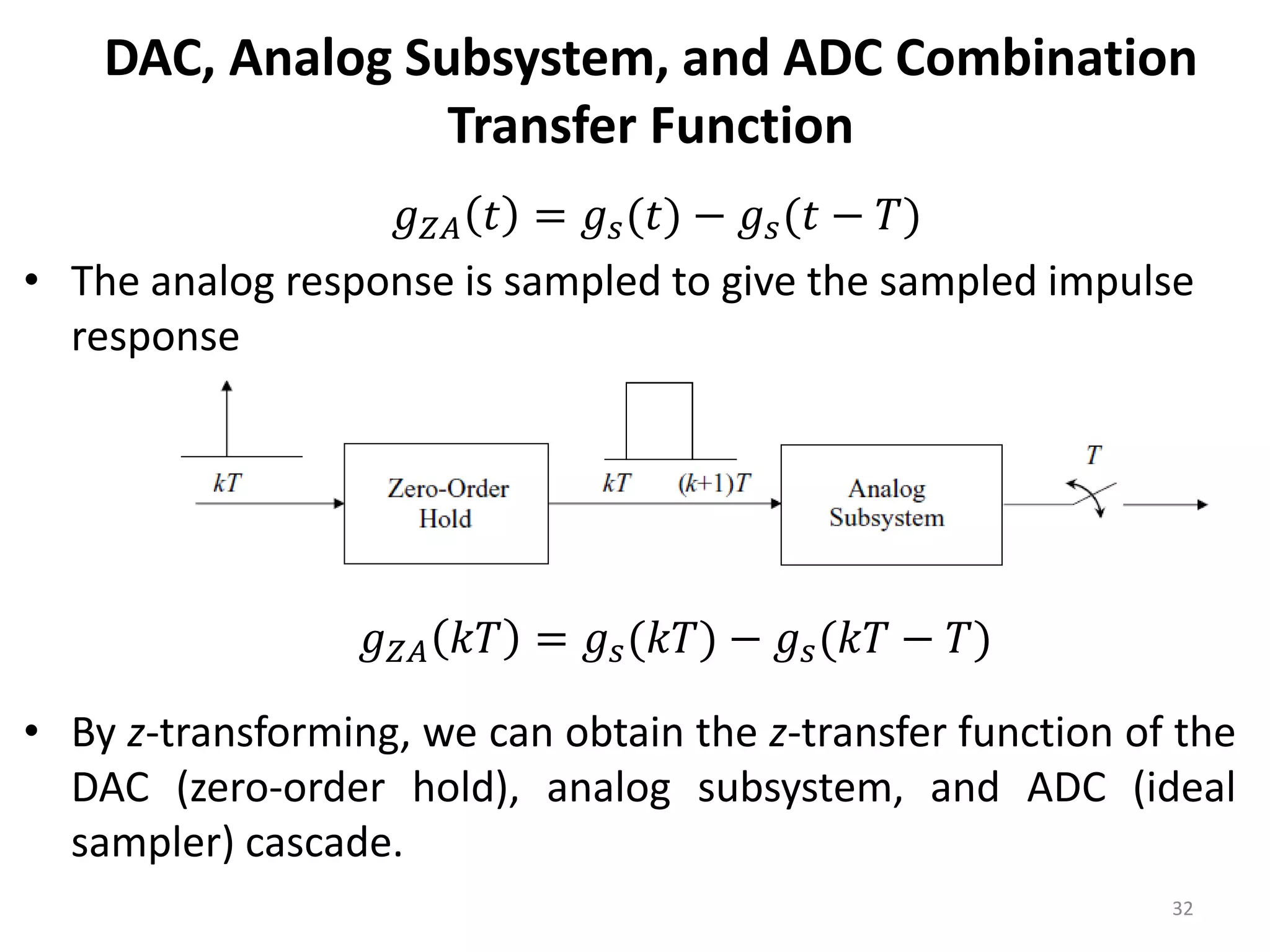
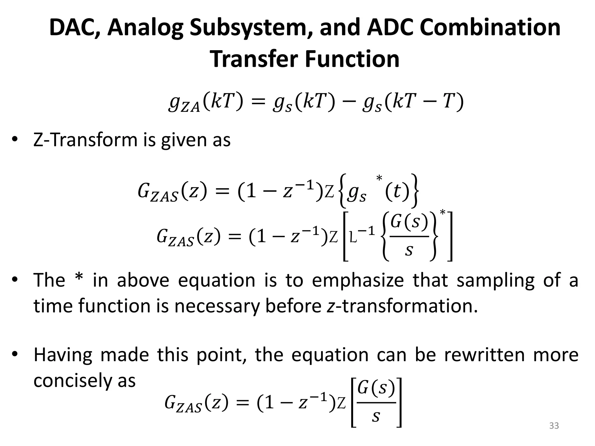
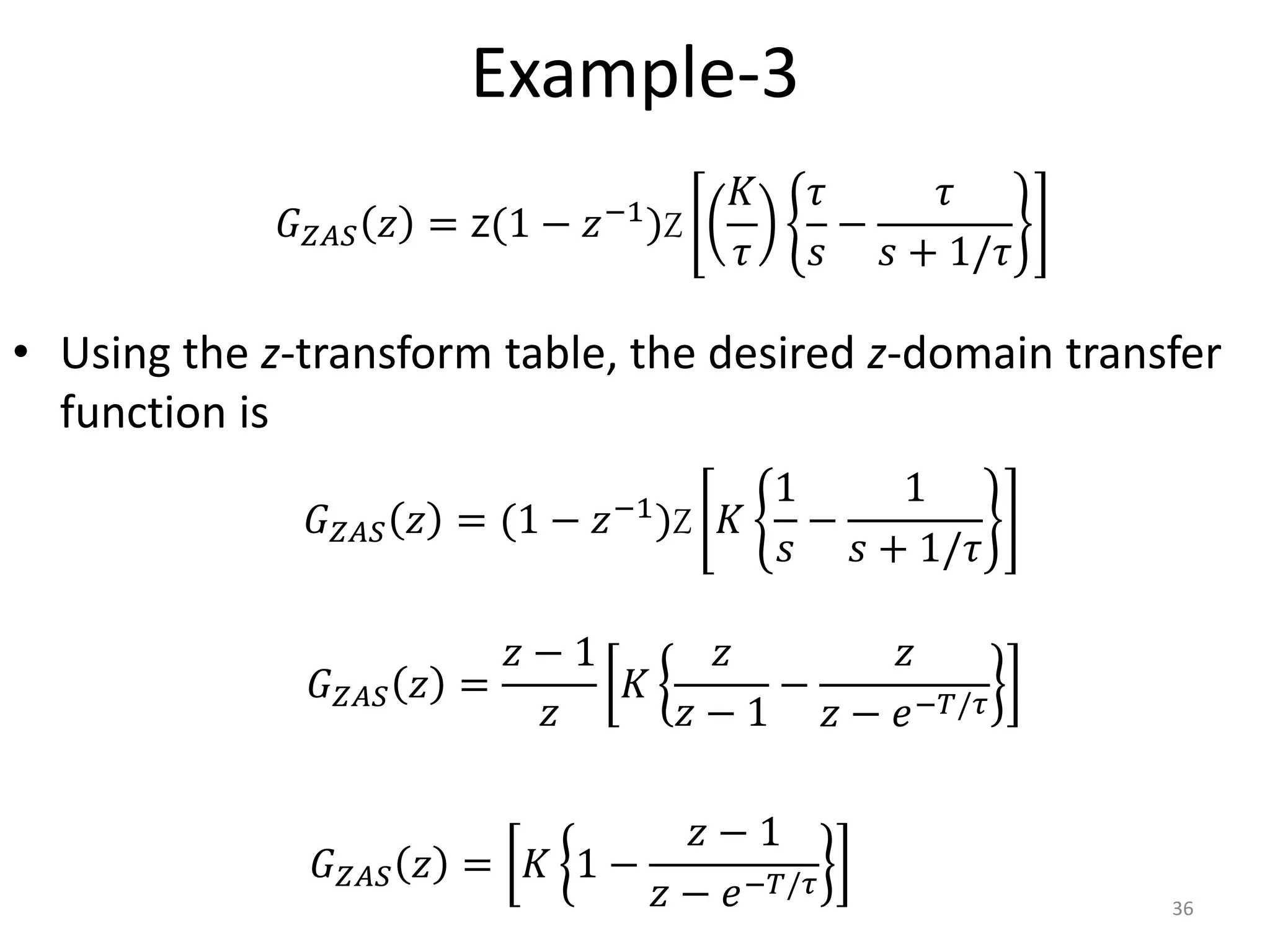
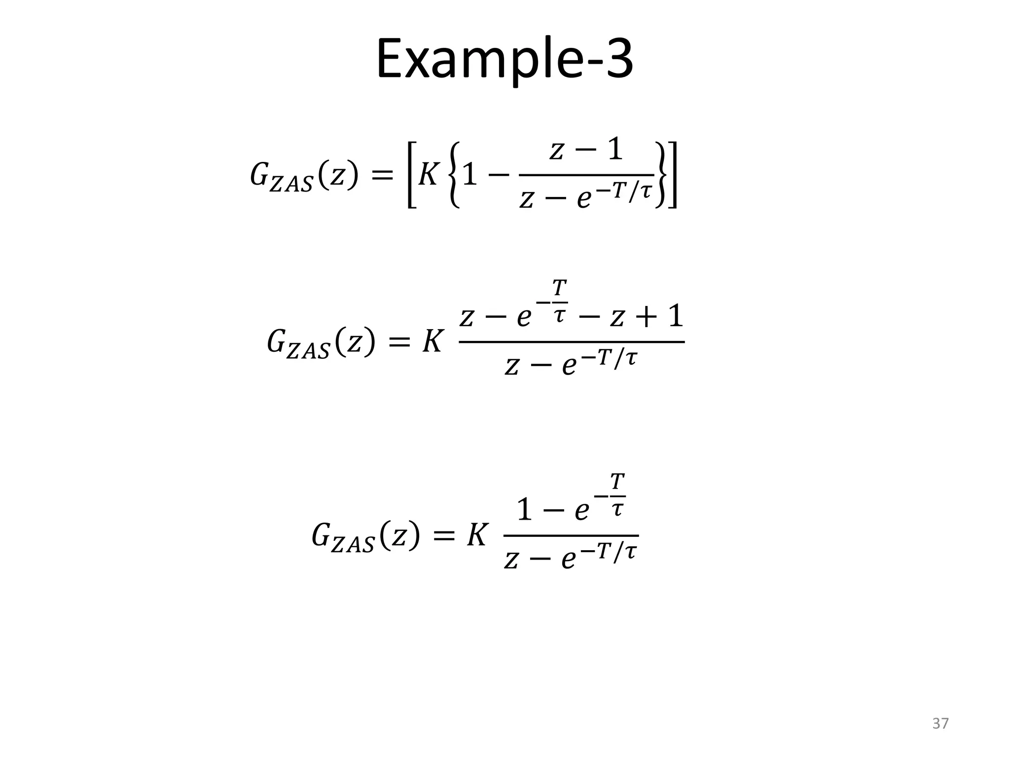
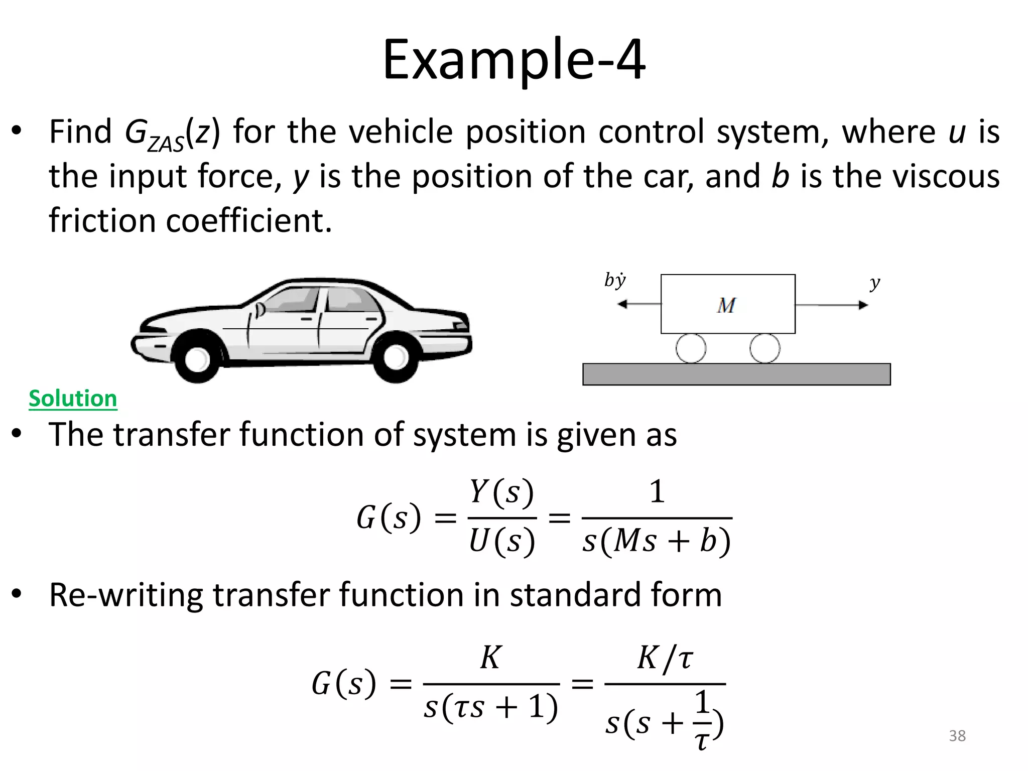
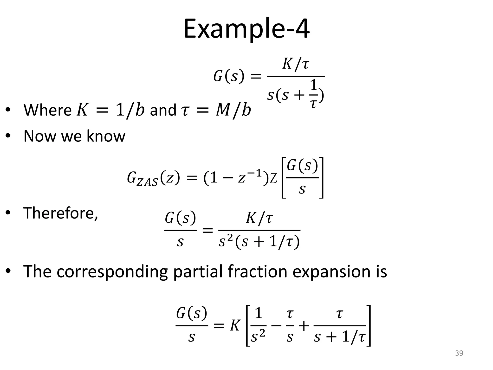
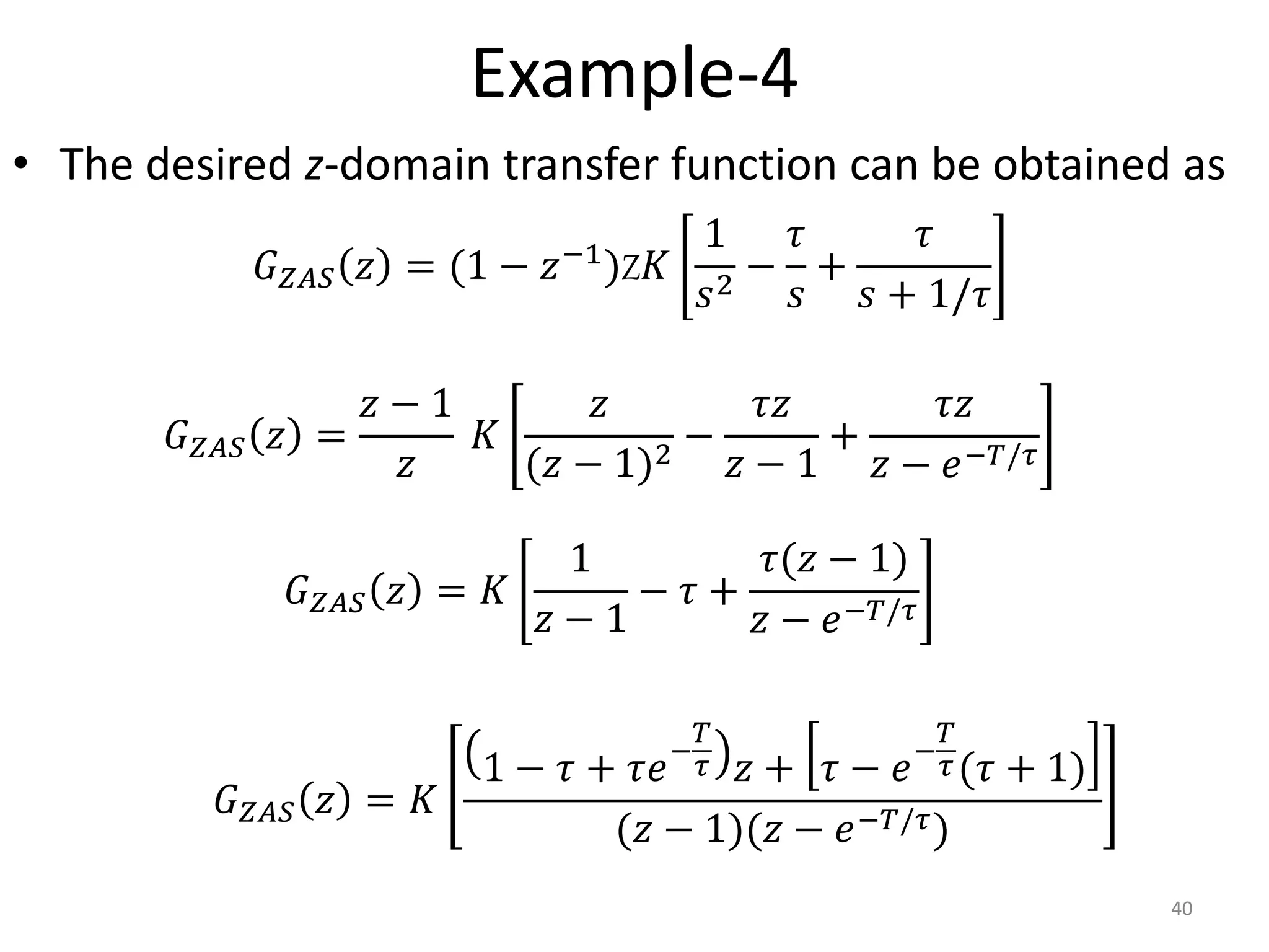
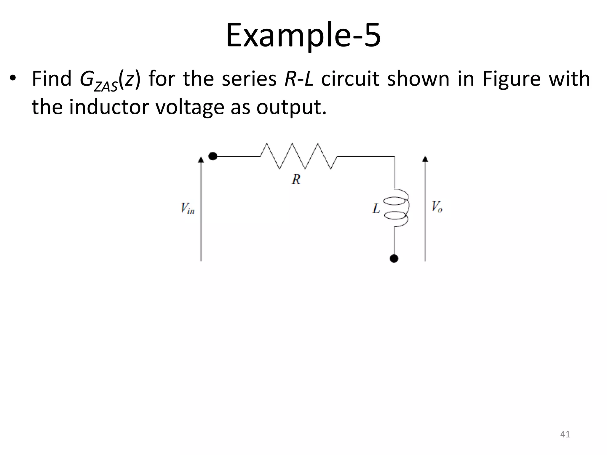
Modern Control Systems (MCS)
Dr. Imtiaz Hussain
Assistant Professor
email: imtiaz.hussain@faculty.muet.edu.pk
URL :http://imtiazhussainkalwar.weebly.com/
Lecture-25-26
Modeling of Digital Control Systems
1
Lecture Outline
• Sampling Theorem
• ADC Model
• DAC Model
• Combined Models
2
Sampling Theorem
• Sampling is necessary for the processing of analog data
using digital elements.
• Successful digital data processing requires that the
samples reflect the nature of the analog signal and that
analog signals be recoverable from a sequence of samples.
3
Sampling Theorem
• Following figure shows two distinct waveforms with
identical samples.
• Obviously, faster sampling of the two waveforms would
produce distinguishable sequences.
4
Sampling Theorem
• Thus, it is obvious that sufficiently fast sampling is a
prerequisite for successful digital data processing.
• The sampling theorem gives a lower bound on the
sampling rate necessary for a given band-limited signal
(i.e., a signal with a known finite bandwidth)
5
Sampling Theorem
• The band limited signal with
• can be reconstructed from the discrete-time waveform
• if and only if the sampling angular frequency 𝜔𝑠 = 2𝜋 𝑇
satisfies the condition
6
𝑓 𝑡
F
𝐹 𝑗𝜔 , 𝐹 𝑗𝜔 ≠ 0, −𝜔𝑚 ≤ 𝜔 ≤ 𝜔𝑚
, 𝐹 𝑗𝜔 = 0, 𝐸𝑙𝑠𝑒𝑤ℎ𝑒𝑟𝑒
𝑓∗
𝑡 =
𝑘=−∞
∞
𝑓 𝑡 𝛿(𝑡 − 𝑘𝑇)
𝜔𝑠 > 2𝜔𝑚
Selection of Sampling Frequency
• A given signal often has a finite “effective bandwidth” beyond
which its spectral components are negligible.
• This allows us to treat physical signals as band limited and
choose a suitable sampling rate for them based on the
sampling theorem.
• In practice, the sampling rate chosen is often larger than the
lower bound specified in the sampling theorem.
• A rule of thumb is to choose 𝜔𝑠 as
7
𝜔𝑠 = 𝑘𝜔𝑚, 5 ≤ 𝑘 ≤ 10
Selection of Sampling Frequency
• The choice of 𝑘 depends on the application.
• In many applications, the upper bound on the sampling
frequency is well below the capabilities of state-of-the-art
hardware.
• A closed-loop control system cannot have a sampling period
below the minimum time required for the output
measurement; that is, the sampling frequency is upper-
bounded by the sensor delay.
8
𝜔𝑠 = 𝑘𝜔𝑚, 5 ≤ 𝑘 ≤ 10
Selection of Sampling Frequency
• For example, oxygen sensors used in automotive air/fuel
ratio control have a sensor delay of about 20 ms, which
corresponds to a sampling frequency upper bound of 50
Hz.
• Another limitation is the computational time needed to
update the control.
• This is becoming less restrictive with the availability of
faster microprocessors but must be considered in
sampling rate selection.
9
Selection of Sampling Frequency
• For a linear system, the output of the system has a spectrum
given by the product of the frequency response and input
spectrum.
• Because the input is not known a priori, we must base our
choice of sampling frequency on the frequency response.
10
Selection of Sampling Frequency (1st Order Systems)
• The frequency response of first order system is
• where K is the DC gain and 𝜔𝑏 is the system bandwidth.
• Time constant and 3db bandwidth relationship
11
𝐻 𝑗𝜔 =
𝐾
𝑗𝜔 𝜔𝑏 + 1
𝜔𝑏 =
1
𝑇
𝑓3𝑑𝑏 =
1
2𝜋𝑇
Selection of Sampling Frequency (1st Order Systems)
12
-30
-25
-20
-15
-10
-5
0
Magnitude
(dB)
System: sys
Frequency (rad/s): 0.33
Magnitude (dB): -2.97
System: sys
Frequency (rad/s): 2.31
Magnitude (dB): -16.9
10
-2
10
-1
10
0
10
1
-90
-45
0
Phase
(deg)
Bode Diagram
Frequency (rad/s)
𝐺 𝑠 =
1
3𝑠 + 1
Selection of Sampling Frequency (1st Order Systems)
• The frequency response amplitude drops below the DC level
by a factor of about 10 at the frequency 7𝜔𝑏.
• If we consider 𝜔𝑚 = 7𝜔𝑏, the sampling frequency is chosen
as
13
𝜔𝑠 = 𝑘𝜔𝑏, 35 ≤ 𝑘 ≤ 70
Selection of Sampling Frequency (2nd Order Systems)
• The frequency response of second order system is
• The bandwidth of the system is approximated by the damped
natural frequency
• Using a frequency of 7𝜔𝑑 as the maximum significant
frequency, we choose the sampling frequency as
14
𝜔𝑠 = 𝑘𝜔𝑑, 35 ≤ 𝑘 ≤ 70
2
)
/
(
1
/
2
)
(
n
n
j
K
j
H








2
1 

 
 n
d
Example-1
• Given a first-order system of bandwidth 10 rad/s, select a
suitable sampling frequency and find the corresponding
sampling period.
• We know
• Choosing k=60
15
Solution
𝜔𝑏 = 10 𝑟𝑎𝑑/𝑠𝑒𝑐
𝜔𝑠 = 𝑘𝜔𝑏, 35 ≤ 𝑘 ≤ 70
𝜔𝑠 = 60𝜔𝑏 = 600 𝑟𝑎𝑑/𝑠𝑒𝑐
Example-1
• Corresponding sapling period is calculated as
16
𝑇 =
2𝜋
𝜔𝑠
=
2 × 3141
600
= 0.01 𝑠𝑒𝑐
Example-2
• A closed-loop control system must be designed for a steady-
state error not to exceed 5 percent, a damping ratio of about
0.7, and an undamped natural frequency of 10 rad/s. Select a
suitable sampling period for the system if the system has a
sensor delay of 0.02 sec.
• Let the sampling frequency be
17
Solution
𝜔𝑠 ≥ 35𝜔𝑑
2
1
35 

 
 n
s
2
7
.
0
1
10
35 


s

Example-2
• The corresponding sampling period is
• A suitable choice is T = 20 ms because this is equal to the
sensor delay.
18
s
rad
s /
95
.
249


𝑇 ≤
2 × 3141
249.95
𝑇 ≤ 0.025 𝑠𝑒𝑐
𝑇 ≤ 25 𝑚𝑠
Home Work
• A closed-loop control system must be designed for a steady-
state error not to exceed 5 percent, a damping ratio of about
0.7, and an undamped natural frequency of 10 rad/s. Select a
suitable sampling period for the system if the system has a
sensor delay of 0.03 sec.
19
Introduction
• A common configuration of digital control system is shown in
following figure.
20
ADC Model
• Assume that
– ADC outputs are exactly equal in magnitude to their inputs
(i.e., quantization errors are negligible)
– The ADC yields a digital output instantaneously
– Sampling is perfectly uniform (i.e., occur at a fixed rate)
• Then the ADC can be modeled as an ideal sampler with
sampling period T.
21
T
t
u*(t)
0
t
u(t)
0
0
t
u*(t)
t
u(t)
0
T
t
δT(t)
0
× =
modulating
pulse(carrier)
modulated
wave
Modulation
signal
u(t) u*(t)





0
*
)
(
)
(
)
(
k
kT
t
t
u
t
u 
Sampling Process
DAC Model
• Assume that
– DAC outputs are exactly equal in magnitude to their inputs.
– The DAC yields an analog output instantaneously.
– DAC outputs are constant over each sampling period.
• Then the input-output relationship of the DAC is given by
23
𝑢 𝑘
𝑍𝑂𝐻
𝑢ℎ 𝑡 = 𝑢 𝑘 , 𝑘𝑇 ≤ 𝑡 ≤ 𝑘 + 1 𝑇
u(k)
u(t)
uh(t)
DAC Model
• Unit impulse response of ZOH
• The transfer function can then be obtained by Laplace
transformation of the impulse response.
24
DAC Model
• As shown in figure the impulse response is a unit pulse of
width T.
• A pulse can be represented as a positive step at time zero
followed by a negative step at time T.
• Using the Laplace transform of a unit step and the time delay
theorem for Laplace transforms,
25
L 𝑢(𝑡) =
1
𝑠
L −𝑢(𝑡 − 𝑇) = −
𝑒−𝑇𝑠
𝑠
DAC Model
• Thus, the transfer function of the ZOH is
26
L 𝑢(𝑡) =
1
𝑠
L −𝑢(𝑡 − 𝑇) = −
𝑒−𝑇𝑠
𝑠
𝐺𝑍𝑂𝐻(𝑠) =
1 − 𝑒−𝑇𝑠
𝑠
DAC, Analog Subsystem, and ADC Combination
Transfer Function
• The cascade of a DAC, analog subsystem, and ADC is shown in
following figure.
• Because both the input and the output of the cascade are
sampled, it is possible to obtain its z-domain transfer function
in terms of the transfer functions of the individual subsystems.
27
DAC, Analog Subsystem, and ADC Combination
Transfer Function
• Using the DAC model, and assuming that the transfer function
of the analog subsystem is G(s), the transfer function of the
DAC and analog subsystem cascade is
28
𝐺𝑍𝐴 𝑠 = 𝐺𝑍𝑂𝐻(𝑠)𝐺(𝑠)
𝐺𝑍𝐴 𝑠 =
1 − 𝑒−𝑇𝑠
𝑠
𝐺(𝑠)
DAC, Analog Subsystem, and ADC Combination
Transfer Function
• The corresponding impulse response is
• The impulse response is the analog system step response
minus a second step response delayed by one sampling
period.
29
𝐺𝑍𝐴 𝑠 =
1 − 𝑒−𝑇𝑠
𝑠
𝐺(𝑠)
𝐺𝑍𝐴 𝑠 =
𝐺(𝑠) − 𝐺(𝑠) 𝑒−𝑇𝑠
𝑠
𝐺𝑍𝐴 𝑠 =
𝐺(𝑠)
𝑠
−
𝐺(𝑠) 𝑒−𝑇𝑠
𝑠
DAC, Analog Subsystem, and ADC Combination
Transfer Function
30
𝐺𝑍𝐴 𝑠 =
𝐺(𝑠)
𝑠
−
𝐺(𝑠) 𝑒−𝑇𝑠
𝑠
DAC, Analog Subsystem, and ADC Combination
Transfer Function
• Inverse Laplace yields
• Where 𝑔𝑠 𝑡 = L−1 𝐺(𝑠)
𝑠
31
𝐺𝑍𝐴 𝑠 =
𝐺(𝑠)
𝑠
−
𝐺(𝑠) 𝑒−𝑇𝑠
𝑠
𝑔𝑍𝐴 𝑡 = 𝑔𝑠(𝑡) − 𝑔𝑠(𝑡 − 𝑇)
DAC, Analog Subsystem, and ADC Combination
Transfer Function
• The analog response is sampled to give the sampled impulse
response
• By z-transforming, we can obtain the z-transfer function of the
DAC (zero-order hold), analog subsystem, and ADC (ideal
sampler) cascade.
32
𝑔𝑍𝐴 𝑡 = 𝑔𝑠(𝑡) − 𝑔𝑠(𝑡 − 𝑇)
𝑔𝑍𝐴 𝑘𝑇 = 𝑔𝑠(𝑘𝑇) − 𝑔𝑠(𝑘𝑇 − 𝑇)
DAC, Analog Subsystem, and ADC Combination
Transfer Function
• Z-Transform is given as
• The * in above equation is to emphasize that sampling of a
time function is necessary before z-transformation.
• Having made this point, the equation can be rewritten more
concisely as
33
𝑔𝑍𝐴 𝑘𝑇 = 𝑔𝑠(𝑘𝑇) − 𝑔𝑠(𝑘𝑇 − 𝑇)
𝐺𝑍𝐴𝑆 𝑧 = (1 − 𝑧−1
)Z 𝑔𝑠
∗
(𝑡)
𝐺𝑍𝐴𝑆 𝑧 = (1 − 𝑧−1
)Z L−1
𝐺(𝑠)
𝑠
∗
𝐺𝑍𝐴𝑆 𝑧 = (1 − 𝑧−1)Z
𝐺(𝑠)
𝑠
Example-3
• Find GZAS(z) for the cruise control system for the vehicle shown
in figure, where u is the input force, v is the velocity of the car,
and b is the viscous friction coefficient.
• The transfer function of system is given as
• Re-writing transfer function in standard form
34
Solution
𝐺 𝑠 =
𝑉(𝑠)
𝑈(𝑠)
=
1
𝑀𝑠 + 𝑏
𝐺 𝑠 =
𝐾
𝜏𝑠 + 1
=
𝐾/𝜏
𝑠 + 1/𝜏
Example-3
• Where 𝐾 = 1/𝑏 and 𝜏 = 𝑀/𝑏
• Now we know
• Therefore,
• The corresponding partial fraction expansion is
35
𝐺 𝑠
𝑠
=
𝐾/𝜏
𝑠(𝑠 + 1/𝜏)
𝐺 𝑠 =
𝐾/𝜏
𝑠 + 1/𝜏
𝐺𝑍𝐴𝑆 𝑧 = (1 − 𝑧−1)Z
𝐺(𝑠)
𝑠
𝐺 𝑠
𝑠
=
𝐾
𝜏
𝜏
𝑠
−
𝜏
𝑠 + 1/𝜏
Example-3
• Using the z-transform table, the desired z-domain transfer
function is
36
𝐺𝑍𝐴𝑆 𝑧 = z(1 − 𝑧−1)Z
𝐾
𝜏
𝜏
𝑠
−
𝜏
𝑠 + 1/𝜏
𝐺𝑍𝐴𝑆 𝑧 = (1 − 𝑧−1)Z 𝐾
1
𝑠
−
1
𝑠 + 1/𝜏
𝐺𝑍𝐴𝑆 𝑧 =
𝑧 − 1
𝑧
𝐾
𝑧
𝑧 − 1
−
𝑧
𝑧 − 𝑒−𝑇/𝜏
𝐺𝑍𝐴𝑆 𝑧 = 𝐾 1 −
𝑧 − 1
𝑧 − 𝑒−𝑇/𝜏
Example-3
37
𝐺𝑍𝐴𝑆 𝑧 = 𝐾 1 −
𝑧 − 1
𝑧 − 𝑒−𝑇/𝜏
𝐺𝑍𝐴𝑆 𝑧 = 𝐾
𝑧 − 𝑒−
𝑇
𝜏 − 𝑧 + 1
𝑧 − 𝑒−𝑇/𝜏
𝐺𝑍𝐴𝑆 𝑧 = 𝐾
1 − 𝑒−
𝑇
𝜏
𝑧 − 𝑒−𝑇/𝜏
Example-4
• Find GZAS(z) for the vehicle position control system, where u is
the input force, y is the position of the car, and b is the viscous
friction coefficient.
• The transfer function of system is given as
• Re-writing transfer function in standard form
38
Solution
𝐺 𝑠 =
𝑌(𝑠)
𝑈(𝑠)
=
1
𝑠(𝑀𝑠 + 𝑏)
𝐺 𝑠 =
𝐾
𝑠(𝜏𝑠 + 1)
=
𝐾/𝜏
𝑠(𝑠 +
1
𝜏
)
𝑦
𝑏𝑦
Example-4
• Where 𝐾 = 1/𝑏 and 𝜏 = 𝑀/𝑏
• Now we know
• Therefore,
• The corresponding partial fraction expansion is
39
𝐺 𝑠
𝑠
=
𝐾/𝜏
𝑠2(𝑠 + 1/𝜏)
𝐺 𝑠 =
𝐾/𝜏
𝑠(𝑠 +
1
𝜏
)
𝐺𝑍𝐴𝑆 𝑧 = (1 − 𝑧−1)Z
𝐺(𝑠)
𝑠
𝐺 𝑠
𝑠
= 𝐾
1
𝑠2
−
𝜏
𝑠
+
𝜏
𝑠 + 1/𝜏
Example-4
• The desired z-domain transfer function can be obtained as
40
𝐺𝑍𝐴𝑆 𝑧 = (1 − 𝑧−1)Z𝐾
1
𝑠2
−
𝜏
𝑠
+
𝜏
𝑠 + 1/𝜏
𝐺𝑍𝐴𝑆 𝑧 =
𝑧 − 1
𝑧
𝐾
𝑧
(𝑧 − 1)2
−
𝜏𝑧
𝑧 − 1
+
𝜏𝑧
𝑧 − 𝑒−𝑇/𝜏
𝐺𝑍𝐴𝑆 𝑧 = 𝐾
1
𝑧 − 1
− 𝜏 +
𝜏(𝑧 − 1)
𝑧 − 𝑒−𝑇/𝜏
𝐺𝑍𝐴𝑆 𝑧 = 𝐾
1 − 𝜏 + 𝜏𝑒−
𝑇
𝜏 𝑧 + 𝜏 − 𝑒−
𝑇
𝜏(𝜏 + 1)
(𝑧 − 1)(𝑧 − 𝑒−𝑇/𝜏)
Example-5
• Find GZAS(z) for the series R-L circuit shown in Figure with
the inductor voltage as output.
41
END OF LECTURES-25-26
To download this lecture visit
http://imtiazhussainkalwar.weebly.com/
42

lecture_25-26__modeling_digital_control_systems.pptx

  • 1.
    Modern Control Systems(MCS) Dr. Imtiaz Hussain Assistant Professor email: imtiaz.hussain@faculty.muet.edu.pk URL :http://imtiazhussainkalwar.weebly.com/ Lecture-25-26 Modeling of Digital Control Systems 1
  • 2.
    Lecture Outline • SamplingTheorem • ADC Model • DAC Model • Combined Models 2
  • 3.
    Sampling Theorem • Samplingis necessary for the processing of analog data using digital elements. • Successful digital data processing requires that the samples reflect the nature of the analog signal and that analog signals be recoverable from a sequence of samples. 3
  • 4.
    Sampling Theorem • Followingfigure shows two distinct waveforms with identical samples. • Obviously, faster sampling of the two waveforms would produce distinguishable sequences. 4
  • 5.
    Sampling Theorem • Thus,it is obvious that sufficiently fast sampling is a prerequisite for successful digital data processing. • The sampling theorem gives a lower bound on the sampling rate necessary for a given band-limited signal (i.e., a signal with a known finite bandwidth) 5
  • 6.
    Sampling Theorem • Theband limited signal with • can be reconstructed from the discrete-time waveform • if and only if the sampling angular frequency 𝜔𝑠 = 2𝜋 𝑇 satisfies the condition 6 𝑓 𝑡 F 𝐹 𝑗𝜔 , 𝐹 𝑗𝜔 ≠ 0, −𝜔𝑚 ≤ 𝜔 ≤ 𝜔𝑚 , 𝐹 𝑗𝜔 = 0, 𝐸𝑙𝑠𝑒𝑤ℎ𝑒𝑟𝑒 𝑓∗ 𝑡 = 𝑘=−∞ ∞ 𝑓 𝑡 𝛿(𝑡 − 𝑘𝑇) 𝜔𝑠 > 2𝜔𝑚
  • 7.
    Selection of SamplingFrequency • A given signal often has a finite “effective bandwidth” beyond which its spectral components are negligible. • This allows us to treat physical signals as band limited and choose a suitable sampling rate for them based on the sampling theorem. • In practice, the sampling rate chosen is often larger than the lower bound specified in the sampling theorem. • A rule of thumb is to choose 𝜔𝑠 as 7 𝜔𝑠 = 𝑘𝜔𝑚, 5 ≤ 𝑘 ≤ 10
  • 8.
    Selection of SamplingFrequency • The choice of 𝑘 depends on the application. • In many applications, the upper bound on the sampling frequency is well below the capabilities of state-of-the-art hardware. • A closed-loop control system cannot have a sampling period below the minimum time required for the output measurement; that is, the sampling frequency is upper- bounded by the sensor delay. 8 𝜔𝑠 = 𝑘𝜔𝑚, 5 ≤ 𝑘 ≤ 10
  • 9.
    Selection of SamplingFrequency • For example, oxygen sensors used in automotive air/fuel ratio control have a sensor delay of about 20 ms, which corresponds to a sampling frequency upper bound of 50 Hz. • Another limitation is the computational time needed to update the control. • This is becoming less restrictive with the availability of faster microprocessors but must be considered in sampling rate selection. 9
  • 10.
    Selection of SamplingFrequency • For a linear system, the output of the system has a spectrum given by the product of the frequency response and input spectrum. • Because the input is not known a priori, we must base our choice of sampling frequency on the frequency response. 10
  • 11.
    Selection of SamplingFrequency (1st Order Systems) • The frequency response of first order system is • where K is the DC gain and 𝜔𝑏 is the system bandwidth. • Time constant and 3db bandwidth relationship 11 𝐻 𝑗𝜔 = 𝐾 𝑗𝜔 𝜔𝑏 + 1 𝜔𝑏 = 1 𝑇 𝑓3𝑑𝑏 = 1 2𝜋𝑇
  • 12.
    Selection of SamplingFrequency (1st Order Systems) 12 -30 -25 -20 -15 -10 -5 0 Magnitude (dB) System: sys Frequency (rad/s): 0.33 Magnitude (dB): -2.97 System: sys Frequency (rad/s): 2.31 Magnitude (dB): -16.9 10 -2 10 -1 10 0 10 1 -90 -45 0 Phase (deg) Bode Diagram Frequency (rad/s) 𝐺 𝑠 = 1 3𝑠 + 1
  • 13.
    Selection of SamplingFrequency (1st Order Systems) • The frequency response amplitude drops below the DC level by a factor of about 10 at the frequency 7𝜔𝑏. • If we consider 𝜔𝑚 = 7𝜔𝑏, the sampling frequency is chosen as 13 𝜔𝑠 = 𝑘𝜔𝑏, 35 ≤ 𝑘 ≤ 70
  • 14.
    Selection of SamplingFrequency (2nd Order Systems) • The frequency response of second order system is • The bandwidth of the system is approximated by the damped natural frequency • Using a frequency of 7𝜔𝑑 as the maximum significant frequency, we choose the sampling frequency as 14 𝜔𝑠 = 𝑘𝜔𝑑, 35 ≤ 𝑘 ≤ 70 2 ) / ( 1 / 2 ) ( n n j K j H         2 1      n d
  • 15.
    Example-1 • Given afirst-order system of bandwidth 10 rad/s, select a suitable sampling frequency and find the corresponding sampling period. • We know • Choosing k=60 15 Solution 𝜔𝑏 = 10 𝑟𝑎𝑑/𝑠𝑒𝑐 𝜔𝑠 = 𝑘𝜔𝑏, 35 ≤ 𝑘 ≤ 70 𝜔𝑠 = 60𝜔𝑏 = 600 𝑟𝑎𝑑/𝑠𝑒𝑐
  • 16.
    Example-1 • Corresponding saplingperiod is calculated as 16 𝑇 = 2𝜋 𝜔𝑠 = 2 × 3141 600 = 0.01 𝑠𝑒𝑐
  • 17.
    Example-2 • A closed-loopcontrol system must be designed for a steady- state error not to exceed 5 percent, a damping ratio of about 0.7, and an undamped natural frequency of 10 rad/s. Select a suitable sampling period for the system if the system has a sensor delay of 0.02 sec. • Let the sampling frequency be 17 Solution 𝜔𝑠 ≥ 35𝜔𝑑 2 1 35      n s 2 7 . 0 1 10 35    s 
  • 18.
    Example-2 • The correspondingsampling period is • A suitable choice is T = 20 ms because this is equal to the sensor delay. 18 s rad s / 95 . 249   𝑇 ≤ 2 × 3141 249.95 𝑇 ≤ 0.025 𝑠𝑒𝑐 𝑇 ≤ 25 𝑚𝑠
  • 19.
    Home Work • Aclosed-loop control system must be designed for a steady- state error not to exceed 5 percent, a damping ratio of about 0.7, and an undamped natural frequency of 10 rad/s. Select a suitable sampling period for the system if the system has a sensor delay of 0.03 sec. 19
  • 20.
    Introduction • A commonconfiguration of digital control system is shown in following figure. 20
  • 21.
    ADC Model • Assumethat – ADC outputs are exactly equal in magnitude to their inputs (i.e., quantization errors are negligible) – The ADC yields a digital output instantaneously – Sampling is perfectly uniform (i.e., occur at a fixed rate) • Then the ADC can be modeled as an ideal sampler with sampling period T. 21 T t u*(t) 0 t u(t) 0
  • 22.
  • 23.
    DAC Model • Assumethat – DAC outputs are exactly equal in magnitude to their inputs. – The DAC yields an analog output instantaneously. – DAC outputs are constant over each sampling period. • Then the input-output relationship of the DAC is given by 23 𝑢 𝑘 𝑍𝑂𝐻 𝑢ℎ 𝑡 = 𝑢 𝑘 , 𝑘𝑇 ≤ 𝑡 ≤ 𝑘 + 1 𝑇 u(k) u(t) uh(t)
  • 24.
    DAC Model • Unitimpulse response of ZOH • The transfer function can then be obtained by Laplace transformation of the impulse response. 24
  • 25.
    DAC Model • Asshown in figure the impulse response is a unit pulse of width T. • A pulse can be represented as a positive step at time zero followed by a negative step at time T. • Using the Laplace transform of a unit step and the time delay theorem for Laplace transforms, 25 L 𝑢(𝑡) = 1 𝑠 L −𝑢(𝑡 − 𝑇) = − 𝑒−𝑇𝑠 𝑠
  • 26.
    DAC Model • Thus,the transfer function of the ZOH is 26 L 𝑢(𝑡) = 1 𝑠 L −𝑢(𝑡 − 𝑇) = − 𝑒−𝑇𝑠 𝑠 𝐺𝑍𝑂𝐻(𝑠) = 1 − 𝑒−𝑇𝑠 𝑠
  • 27.
    DAC, Analog Subsystem,and ADC Combination Transfer Function • The cascade of a DAC, analog subsystem, and ADC is shown in following figure. • Because both the input and the output of the cascade are sampled, it is possible to obtain its z-domain transfer function in terms of the transfer functions of the individual subsystems. 27
  • 28.
    DAC, Analog Subsystem,and ADC Combination Transfer Function • Using the DAC model, and assuming that the transfer function of the analog subsystem is G(s), the transfer function of the DAC and analog subsystem cascade is 28 𝐺𝑍𝐴 𝑠 = 𝐺𝑍𝑂𝐻(𝑠)𝐺(𝑠) 𝐺𝑍𝐴 𝑠 = 1 − 𝑒−𝑇𝑠 𝑠 𝐺(𝑠)
  • 29.
    DAC, Analog Subsystem,and ADC Combination Transfer Function • The corresponding impulse response is • The impulse response is the analog system step response minus a second step response delayed by one sampling period. 29 𝐺𝑍𝐴 𝑠 = 1 − 𝑒−𝑇𝑠 𝑠 𝐺(𝑠) 𝐺𝑍𝐴 𝑠 = 𝐺(𝑠) − 𝐺(𝑠) 𝑒−𝑇𝑠 𝑠 𝐺𝑍𝐴 𝑠 = 𝐺(𝑠) 𝑠 − 𝐺(𝑠) 𝑒−𝑇𝑠 𝑠
  • 30.
    DAC, Analog Subsystem,and ADC Combination Transfer Function 30 𝐺𝑍𝐴 𝑠 = 𝐺(𝑠) 𝑠 − 𝐺(𝑠) 𝑒−𝑇𝑠 𝑠
  • 31.
    DAC, Analog Subsystem,and ADC Combination Transfer Function • Inverse Laplace yields • Where 𝑔𝑠 𝑡 = L−1 𝐺(𝑠) 𝑠 31 𝐺𝑍𝐴 𝑠 = 𝐺(𝑠) 𝑠 − 𝐺(𝑠) 𝑒−𝑇𝑠 𝑠 𝑔𝑍𝐴 𝑡 = 𝑔𝑠(𝑡) − 𝑔𝑠(𝑡 − 𝑇)
  • 32.
    DAC, Analog Subsystem,and ADC Combination Transfer Function • The analog response is sampled to give the sampled impulse response • By z-transforming, we can obtain the z-transfer function of the DAC (zero-order hold), analog subsystem, and ADC (ideal sampler) cascade. 32 𝑔𝑍𝐴 𝑡 = 𝑔𝑠(𝑡) − 𝑔𝑠(𝑡 − 𝑇) 𝑔𝑍𝐴 𝑘𝑇 = 𝑔𝑠(𝑘𝑇) − 𝑔𝑠(𝑘𝑇 − 𝑇)
  • 33.
    DAC, Analog Subsystem,and ADC Combination Transfer Function • Z-Transform is given as • The * in above equation is to emphasize that sampling of a time function is necessary before z-transformation. • Having made this point, the equation can be rewritten more concisely as 33 𝑔𝑍𝐴 𝑘𝑇 = 𝑔𝑠(𝑘𝑇) − 𝑔𝑠(𝑘𝑇 − 𝑇) 𝐺𝑍𝐴𝑆 𝑧 = (1 − 𝑧−1 )Z 𝑔𝑠 ∗ (𝑡) 𝐺𝑍𝐴𝑆 𝑧 = (1 − 𝑧−1 )Z L−1 𝐺(𝑠) 𝑠 ∗ 𝐺𝑍𝐴𝑆 𝑧 = (1 − 𝑧−1)Z 𝐺(𝑠) 𝑠
  • 34.
    Example-3 • Find GZAS(z)for the cruise control system for the vehicle shown in figure, where u is the input force, v is the velocity of the car, and b is the viscous friction coefficient. • The transfer function of system is given as • Re-writing transfer function in standard form 34 Solution 𝐺 𝑠 = 𝑉(𝑠) 𝑈(𝑠) = 1 𝑀𝑠 + 𝑏 𝐺 𝑠 = 𝐾 𝜏𝑠 + 1 = 𝐾/𝜏 𝑠 + 1/𝜏
  • 35.
    Example-3 • Where 𝐾= 1/𝑏 and 𝜏 = 𝑀/𝑏 • Now we know • Therefore, • The corresponding partial fraction expansion is 35 𝐺 𝑠 𝑠 = 𝐾/𝜏 𝑠(𝑠 + 1/𝜏) 𝐺 𝑠 = 𝐾/𝜏 𝑠 + 1/𝜏 𝐺𝑍𝐴𝑆 𝑧 = (1 − 𝑧−1)Z 𝐺(𝑠) 𝑠 𝐺 𝑠 𝑠 = 𝐾 𝜏 𝜏 𝑠 − 𝜏 𝑠 + 1/𝜏
  • 36.
    Example-3 • Using thez-transform table, the desired z-domain transfer function is 36 𝐺𝑍𝐴𝑆 𝑧 = z(1 − 𝑧−1)Z 𝐾 𝜏 𝜏 𝑠 − 𝜏 𝑠 + 1/𝜏 𝐺𝑍𝐴𝑆 𝑧 = (1 − 𝑧−1)Z 𝐾 1 𝑠 − 1 𝑠 + 1/𝜏 𝐺𝑍𝐴𝑆 𝑧 = 𝑧 − 1 𝑧 𝐾 𝑧 𝑧 − 1 − 𝑧 𝑧 − 𝑒−𝑇/𝜏 𝐺𝑍𝐴𝑆 𝑧 = 𝐾 1 − 𝑧 − 1 𝑧 − 𝑒−𝑇/𝜏
  • 37.
    Example-3 37 𝐺𝑍𝐴𝑆 𝑧 =𝐾 1 − 𝑧 − 1 𝑧 − 𝑒−𝑇/𝜏 𝐺𝑍𝐴𝑆 𝑧 = 𝐾 𝑧 − 𝑒− 𝑇 𝜏 − 𝑧 + 1 𝑧 − 𝑒−𝑇/𝜏 𝐺𝑍𝐴𝑆 𝑧 = 𝐾 1 − 𝑒− 𝑇 𝜏 𝑧 − 𝑒−𝑇/𝜏
  • 38.
    Example-4 • Find GZAS(z)for the vehicle position control system, where u is the input force, y is the position of the car, and b is the viscous friction coefficient. • The transfer function of system is given as • Re-writing transfer function in standard form 38 Solution 𝐺 𝑠 = 𝑌(𝑠) 𝑈(𝑠) = 1 𝑠(𝑀𝑠 + 𝑏) 𝐺 𝑠 = 𝐾 𝑠(𝜏𝑠 + 1) = 𝐾/𝜏 𝑠(𝑠 + 1 𝜏 ) 𝑦 𝑏𝑦
  • 39.
    Example-4 • Where 𝐾= 1/𝑏 and 𝜏 = 𝑀/𝑏 • Now we know • Therefore, • The corresponding partial fraction expansion is 39 𝐺 𝑠 𝑠 = 𝐾/𝜏 𝑠2(𝑠 + 1/𝜏) 𝐺 𝑠 = 𝐾/𝜏 𝑠(𝑠 + 1 𝜏 ) 𝐺𝑍𝐴𝑆 𝑧 = (1 − 𝑧−1)Z 𝐺(𝑠) 𝑠 𝐺 𝑠 𝑠 = 𝐾 1 𝑠2 − 𝜏 𝑠 + 𝜏 𝑠 + 1/𝜏
  • 40.
    Example-4 • The desiredz-domain transfer function can be obtained as 40 𝐺𝑍𝐴𝑆 𝑧 = (1 − 𝑧−1)Z𝐾 1 𝑠2 − 𝜏 𝑠 + 𝜏 𝑠 + 1/𝜏 𝐺𝑍𝐴𝑆 𝑧 = 𝑧 − 1 𝑧 𝐾 𝑧 (𝑧 − 1)2 − 𝜏𝑧 𝑧 − 1 + 𝜏𝑧 𝑧 − 𝑒−𝑇/𝜏 𝐺𝑍𝐴𝑆 𝑧 = 𝐾 1 𝑧 − 1 − 𝜏 + 𝜏(𝑧 − 1) 𝑧 − 𝑒−𝑇/𝜏 𝐺𝑍𝐴𝑆 𝑧 = 𝐾 1 − 𝜏 + 𝜏𝑒− 𝑇 𝜏 𝑧 + 𝜏 − 𝑒− 𝑇 𝜏(𝜏 + 1) (𝑧 − 1)(𝑧 − 𝑒−𝑇/𝜏)
  • 41.
    Example-5 • Find GZAS(z)for the series R-L circuit shown in Figure with the inductor voltage as output. 41
  • 42.
    END OF LECTURES-25-26 Todownload this lecture visit http://imtiazhussainkalwar.weebly.com/ 42