Hell-If-I-Know

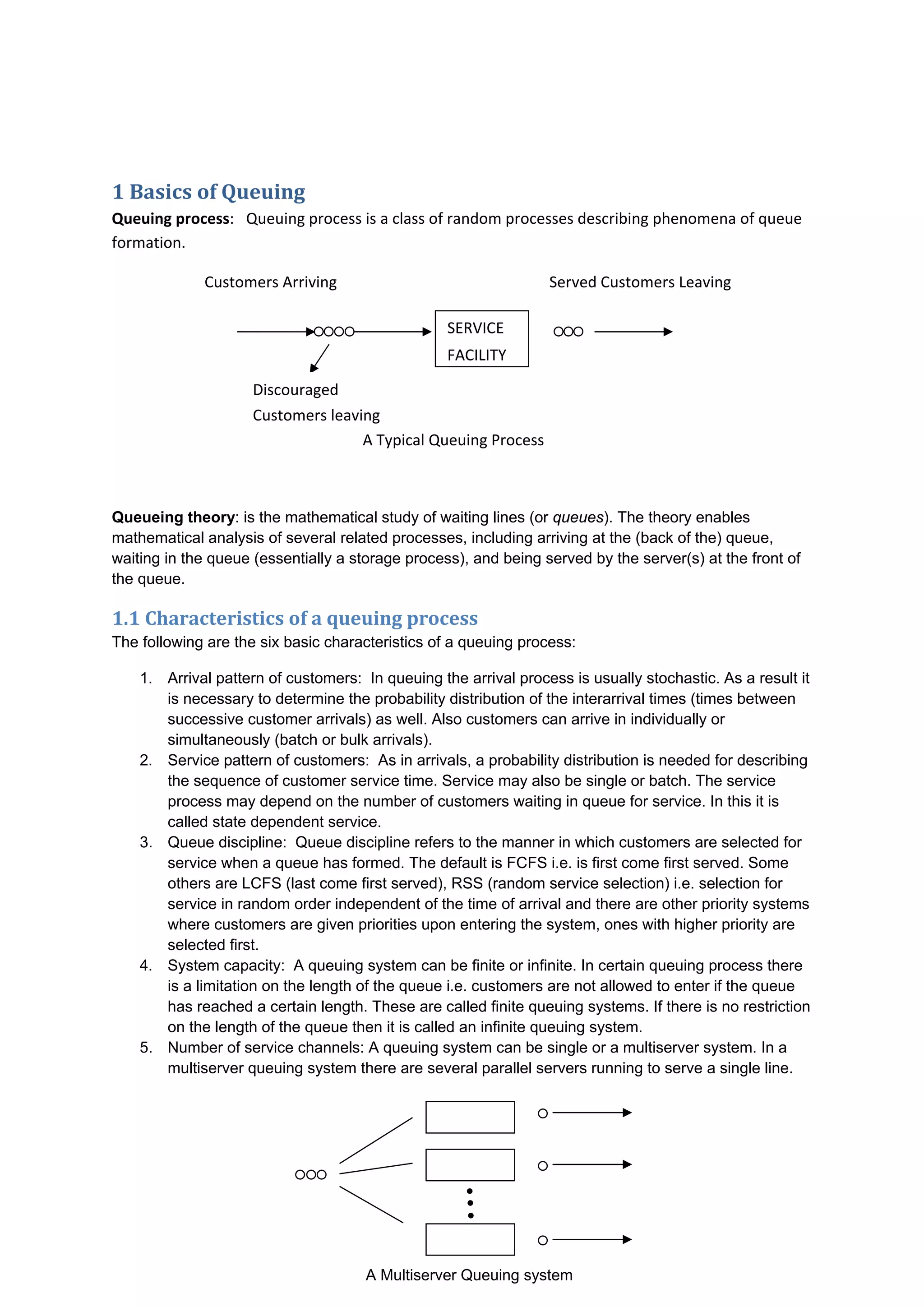
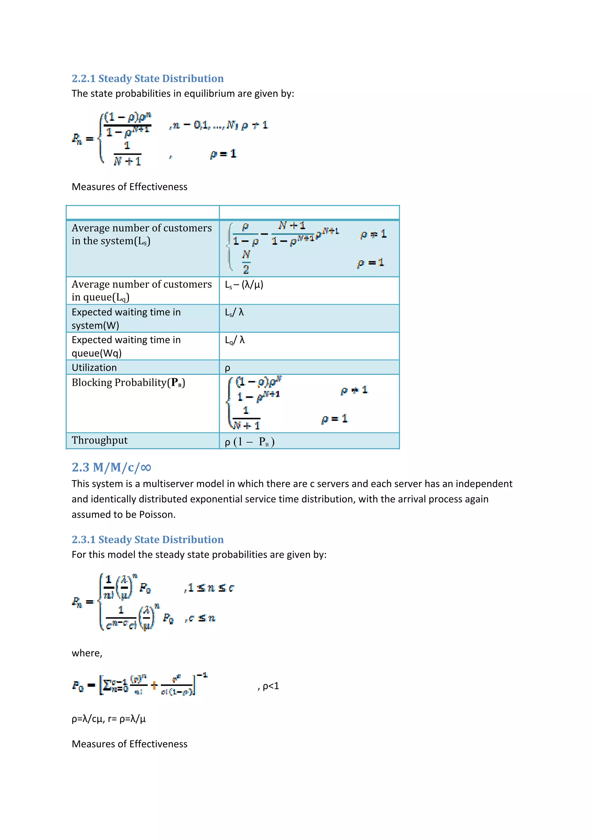
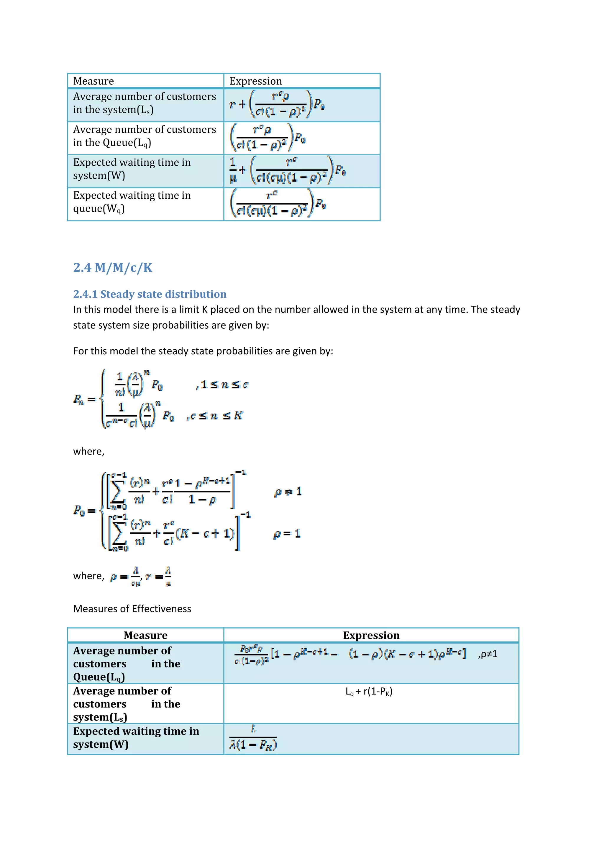
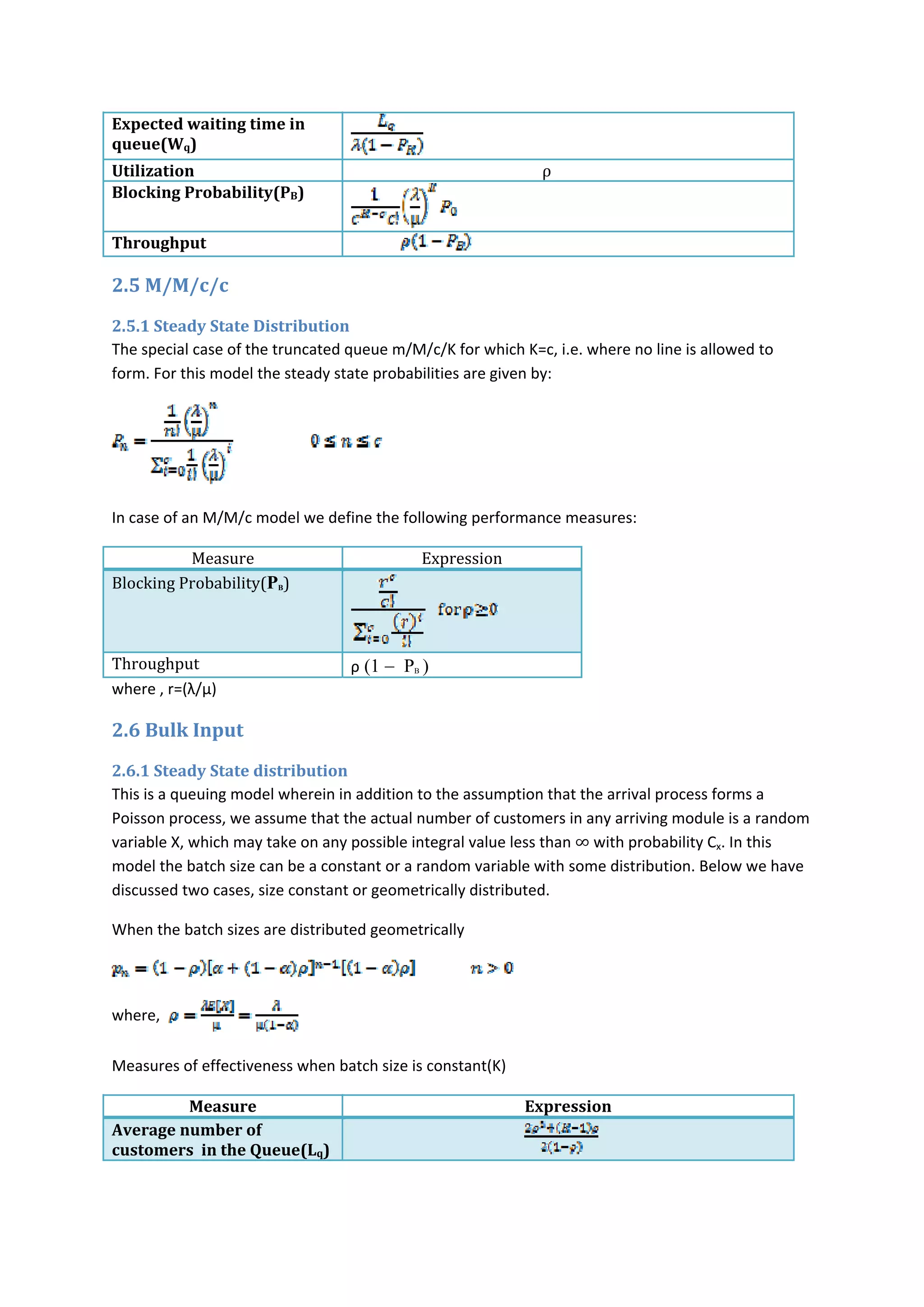
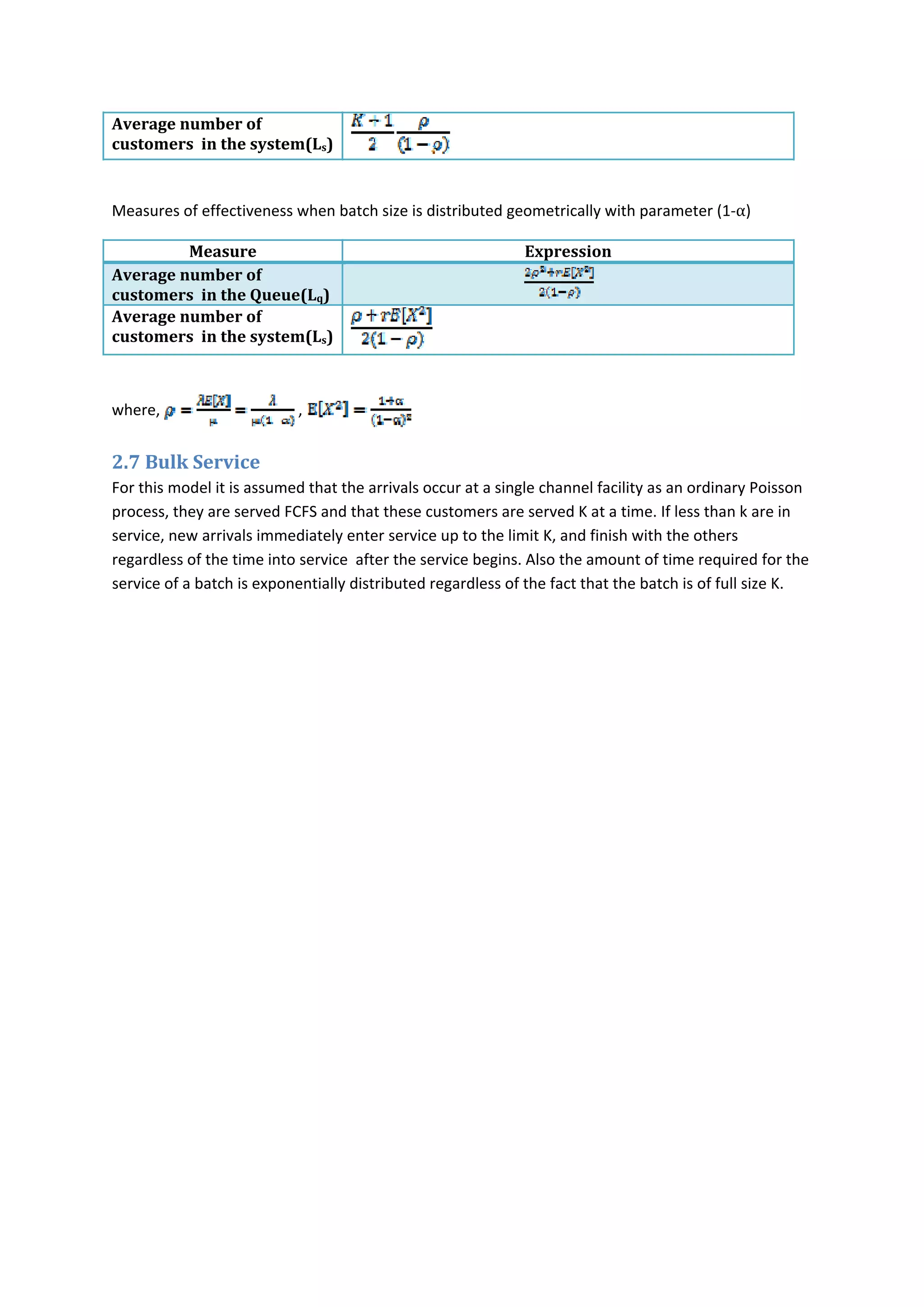
1. Contents
1 Basics of Queuing ................................................................................................................................. 2
1.1 Characteristics of a queuing process ............................................................................................ 2
1.2 Poisson Process and Exponential Distribution .............................................................................. 3
1.3 Markov process ............................................................................................................................. 4
2 Markovian Queuing Models ................................................................................................................. 5
2.1 M/M/1/∞ ...................................................................................................................................... 5
2.1.1 Steady State Distribution ....................................................................................................... 6
2.1.2 Transient solution .................................................................................................................. 6
2.2 M/M/1/N ...................................................................................................................................... 6
2.2.1 Steady State Distribution ....................................................................................................... 7
2.3 M/M/c/∞ ...................................................................................................................................... 7
2.3.1 Steady State Distribution ....................................................................................................... 7
2.4 M/M/c/k ........................................................................................................................................ 8
2.4.1 Steady state distribution ........................................................................................................ 8
2.5 M/M/c/c ........................................................................................................................................ 9
2.5.1 Steady State Distribution ....................................................................................................... 9
2.6 Bulk Input ...................................................................................................................................... 9
2.6.1 Steady State distribution ....................................................................................................... 9
2.7 Bulk Service ................................................................................................................................. 10
GLOSSARY.............................................................................................................................................. 11

2.
1 Basics of Queuing
Queuing process: Queuing process is a class of random processes describing phenomena of queue
formation.
Customers Arriving Served Customers Leaving
SERVICE
FACILITY
A Typical Queuing Process
Discouraged
Customers leaving
Queueing theory: is the mathematical study of waiting lines (or queues). The theory enables
mathematical analysis of several related processes, including arriving at the (back of the) queue,
waiting in the queue (essentially a storage process), and being served by the server(s) at the front of
the queue.
1.1 Characteristics of a queuing process
The following are the six basic characteristics of a queuing process:
1. Arrival pattern of customers: In queuing the arrival process is usually stochastic. As a result it
is necessary to determine the probability distribution of the interarrival times (times between
successive customer arrivals) as well. Also customers can arrive in individually or
simultaneously (batch or bulk arrivals).
2. Service pattern of customers: As in arrivals, a probability distribution is needed for describing
the sequence of customer service time. Service may also be single or batch. The service
process may depend on the number of customers waiting in queue for service. In this it is
called state dependent service.
3. Queue discipline: Queue discipline refers to the manner in which customers are selected for
service when a queue has formed. The default is FCFS i.e. is first come first served. Some
others are LCFS (last come first served), RSS (random service selection) i.e. selection for
service in random order independent of the time of arrival and there are other priority systems
where customers are given priorities upon entering the system, ones with higher priority are
selected first.
4. System capacity: A queuing system can be finite or infinite. In certain queuing process there
is a limitation on the length of the queue i.e. customers are not allowed to enter if the queue
has reached a certain length. These are called finite queuing systems. If there is no restriction
on the length of the queue then it is called an infinite queuing system.
5. Number of service channels: A queuing system can be single or a multiserver system. In a
multiserver queuing system there are several parallel servers running to serve a single line.
A Multiserver Queuing system

3. 6. Number of service stages: A queuing system may have only a single stage of service. But as
an example of a multistage queuing system consider the physical examination procedure,
where each patient proceeds through various stages of medical examination, like throat check
up, eye test, blood test etc.
Kendall’s notation
A queuing process can be described using a notation which uses series of symbols and slashes such
as A/B/X/Y/Z, where
A: indicates the interarrival time distribution
B: indicates the service time distribution
X: the number of parallel servers
Y: the restriction on system capacity
Z: the queue discipline
Standard symbols for the characteristics A and B
M
D
EK
HK
PH
G
Exponential
Deterministic
Erlang type k
Mixture of k exponentials
Phase type
General
1.2 Poisson Process and Exponential Distribution
The most common stochastic models assume that the arrival rate and service rate follow a poisson
distribution.
The Poisson process is a counting process {N(t),t≥0}, where N(t) denotes the total number of arrivals
up to time t with N(0)=0 and which satisfies the following three assumptions:
i. The probability that an arrival occurs between time t and t+∆t is equal to λ∆t+o(∆t),
where λ is a constant independent of N(t) and
= 0
ii. Pr{more than one arrival between t and t+∆t }= o(∆t)
iii. The number of arrivals in nonoverlapping intervals is independent, i.e. the
process has independent increments.
Stationary increments: One of the most important properties of Poisson process is that the
number of occurrences in intervals of equal width are identically distributed. In particular,
for t>s, the difference N(t) – N(s) is identically distributed as N(t+h) – N(s+h).

4.
Now, if the arrival process is Poisson then it can be easily shown that the associated random
variable defined as the time between successive arrivals (interarrival time) follows the
exponential distribution. Likewise if the interarrival times are independent and have the
same exponential distribution , then the arrival rate follows a Poisson distribution.
The above theory also holds for service rate and service times.
Markovian property of the exponential distribution: A stochastic process has the Markov
property if the conditional probability distribution of future states of the process depends
only upon the present state; that is, given the present, the future does not depend on the
past. For service times this property states that the probability that a customer currently in service
has t units of remaining service is independent of how long it has already been in service. Thus we
have,
Pr{T≤t1|T≥t0} = Pr{0≤T≤t1-t0}
Stationary process (or strict(ly) stationary process) is a stochastic process whose joint probability
distribution does not change when shifted in time or space i.e.
If Xt is a stochastic process then Xt is said to be stationary if, for all k, for all τ, and for all,
t1,t2,...tk
1.3 Markov process
Markov process, named after the Russian mathematician Andrey Markov, is a time-varying random
phenomenon for which a specific property the Markov property holds.
Markov Chain: If we assume that the state space, I, is discrete, then the Markov process is known as
a Markov Chain
DTMC(Discrete Time Markov Chain): If the parametric space , T, is also discrete, then the Markov
chain is known as a discrete time Markov chain. In this case we let T= {0,1,2,...}. For a DTMC the
Markov propert can be stated as
P (Xn=in|X0=i0,X1=i1,...,Xn‐1=in‐1) = P (Xn=in|Xn‐1=in‐1), i0,i1,...,in є I
CTMC(Continuous Time Markov Chain): If the parametric space, T, is continuous, then the Markov
chain is called a continuous time Markov chain. In this case we let T= [0,∞). For a CTMC the Markov
property can be stated as
P (X(t)=x|X(tn)=xn,X(tn‐1)=xn‐1,...,X(t0)=x0) = P (X(t)=x | X(tn)=xn)
1.4 Birth‐death process
The birth‐death process is a special case of CTMC where the states represent the current
size of a population and where the transitions are limited to births and deaths. Birth‐death

5. processes have many applications in demography, queueing theory, performance
engineering, or in biology.
When a birth occurs, the process goes from state n to n+1. When a death occurs, the
process goes from state n to state n‐1. The process is specified by birth rates
and death rates .
Examples
A pure birth process is a birth-death process where μi = 0 for all .
A pure death process is a birth-death process where λi = 0 for all .
A (homogeneous) Poisson process is a pure birth process where λi = λ for all
M/M/1 model and M/M/c model, both used in queueing theory, are birth-death processes
used to describe customers in an infinite queue.
2 Markovian Queuing Models
2.1 M/M/1/∞
The M/M/1 queuing system is described as a queuing model where:
arrivals are a Poisson process i.e. interarrival time is exponentially distributed;
service time is exponentially distributed;
there is one server;
the length of queue in which arriving users wait before being served is infinite;
the population of users (i.e. the pool of users) available to join the system is infinite
λ
3 2 1
µ

6.
A simple M/M/1 queue with arrival rate λ and service rate µ
2.1.1 Steady State Distribution
Let pn represents the probability mass function of a discrete random variable denoting the number
of customers in the system in long run
pn = (1‐ρ) ρn
, ρ<1
where,
ρ =λ/µ represents the traffic intensity of the system. For a stable system the intensity ρ must be less
than 1.
It can be seen above that the steady state probabilities for an M/M/1 queue follows the geometric
distribution with parameter (1‐ ρ)
Measures of Effectiveness
Measure Expression
Average number of
customers in the system(Ls)
ρ/(1‐ ρ)
Average number of
customers in the Queue(Lq)
ρ2
/(1‐ ρ)
Expected waiting time in
system(W)
1/(µ‐λ)
Expected waiting time in
queue(Wq)
ρ/( µ‐λ)
Utilization Ρ
2.1.2 Transient solution
The transient probabilities pn(t)=Pr{X(t)=n} for an M/M/1 queue are given by
for all n≥0, where
is the infinite series for the modified Bessel function of the first kind.
2.2 M/M/1/N
This system is a type of M/M/1/∞ queue with at most N(+ve integer ) customers allowed in the
system.

7. 2.2.1 Steady State Distribution
The state probabilities in equilibrium are given by:
Measures of Effectiveness
Measure Expression
Average number of customers
in the system(Ls)
Average number of customers
in queue(Lq)
Ls – (λ/µ)
Expected waiting time in
system(W)
Ls/ λ
Expected waiting time in
queue(Wq)
Lq/ λ
Utilization ρ
Blocking Probability(PB)
Throughput ρ (1 − PB )
2.3 M/M/c/∞
This system is a multiserver model in which there are c servers and each server has an independent
and identically distributed exponential service time distribution, with the arrival process again
assumed to be Poisson.
2.3.1 Steady State Distribution
For this model the steady state probabilities are given by:
where,
, ρ<1
ρ=λ/cµ, r= ρ=λ/µ
Measures of Effectiveness

8. Measure Expression
Average number of customers
in the system(Ls)
Average number of customers
in the Queue(Lq)
Expected waiting time in
system(W)
Expected waiting time in
queue(Wq)
2.4 M/M/c/K
2.4.1 Steady state distribution
In this model there is a limit K placed on the number allowed in the system at any time. The steady
state system size probabilities are given by:
For this model the steady state probabilities are given by:
where,
where, ,
Measures of Effectiveness
Measure Expression
Average number of
customers in the
Queue(Lq)
,ρ≠1
Average number of
customers in the
system(Ls)
Lq + r(1‐PK)
Expected waiting time in
system(W)

9. Expected waiting time in
queue(Wq)
Utilization ρ
Blocking Probability(PB)
Throughput
2.5 M/M/c/c
2.5.1 Steady State Distribution
The special case of the truncated queue m/M/c/K for which K=c, i.e. where no line is allowed to
form. For this model the steady state probabilities are given by:
In case of a model we define the fol rmance measures: n M/M/c lowing perfo
Measure Expression
Blocking Probability(PB)
Throughput ρ (1 − PB )
where , r=(λ/µ)
2.6 Bulk Input
2.6.1 Steady State distribution
This is a queuing model wherein in addition to the assumption that the arrival process forms a
Poisson process, we assume that the actual number of customers in any arriving module is a random
variable X, which may take on any possible integral value less than ∞ with probability Cx. In this
model the batch size can be a constant or a random variable with some distribution. Below we have
discussed two cases, size constant or geometrically distributed.
When the batch sizes are distributed geometrically
where,
Measures of effectiveness when batch size is constant(K)
Measure Expression
Average number of
customers in the Queue(Lq)

10. Average number of
customers in the system(Ls)
Measures of effectiveness when batch size is distributed geometrically with parameter (1‐α)
Measure Expression
Average number of
customers in the Queue(Lq)
Average number of
customers in the system(Ls)
where, ,
2.7 Bulk Service
For this model it is assumed that the arrivals occur at a single channel facility as an ordinary Poisson
process, they are served FCFS and that these customers are served K at a time. If less than k are in
service, new arrivals immediately enter service up to the limit K, and finish with the others
regardless of the time into service after the service begins. Also the amount of time required for the
service of a batch is exponentially distributed regardless of the fact that the batch is of full size K.

11. GLOSSARY
Arrival rate (λ): Average rate at which customers arrive to the system. Has units of "customers /
time unit".
Blocking Probability: Blocking probability gives the probability of the event that an arrival finds all
servers busy and leaves without service.
FIFO: First in, first out (FIFO) queuing is the most basic queue scheduling discipline. In FIFO queuing,
all packets are treated equally by placing them into a single queue, and then servicing them in the
same order that they were placed into the queue. FIFO queuing is also referred to as First come, first
served (FCFS) queuing.
LIFO: The LIFO Queue model supports the last‐in, first‐out (LIFO) queuing discipline. The entity that
departs from the queue at a given time is the most recent arrival.
M/M/1 model: A queuing model with one server and arrival and service time exponentially
distributed.
M/M/c model: A queuing model with c servers and arrival and service time exponentially
distributed.
M/M/1/N model: A queuing model with 1 server, system capacity N and arrival and service time
exponentially distributed.
M/M/c/K model: A queuing model with c servers, system capacity K and arrival and service time
exponentially distributed
Orbit: Queuing systems with retrial of the attempts are characterized by the fact that an arrival
customer who finds the server occupied is obliged to join a group of blocked customers, called orbit,
and reapply after random intervals of time to obtain the service.
Queuing delay: is the time a job waits in queue until it can be executed.
Queuing model: is used to approximate a real queuing situation or system, so the queuing behaviour
can be analysed mathematically. Queuing models help measure a number of useful steady
state performance measures including the average number in the queue, or the system, average
time spent in the queue, or the system, distribution of waiting times, the probability the queue is
full, or empty, and the probability of finding the system in a particular state.
Retrial queues: Many queuing systems have the feature that, customers who find all servers busy
upon arrival are obliged to leave the service area and come back to the system after a random
amount of time
Sample Path: A sample path for the stochastic process {Xt: t є T} is the function on T to the range of
the process which assigns to each t the value Xt(w), where w is a previously given fixed point in the
domain of the process.

12. Service Rate (µ): The average rate at which an individual server can serve customers. Has units of
"customers / time unit" and is the reciprocal of the average time it takes to serve one customer.
Service Discipline: Queue discipline or service discipline refers to the manner in which customers are
selected for service when a queue has formed like FIFO/FCFS, LIFO etc.
Servers: The number of servers available to serve customers entering a queuing system. The number
of servers must be a whole number that is greater than or equal to one.
Steady State: The state of the system after it has been in operation for a long time.
System Capacity: The total number of customers that can be in the system, either waiting or being
served. Must be a whole number that is greater than or equal to one.
Traffic Intensity: Traffic intensity is a measure of the average occupancy of a server or resource
during a specified period of time.
Throughput: is the number of customers served per unit time
Utilization: The proportion of time a server is busy is the server utilization.
Waiting Times: Customer waiting time can be of two types, the time the customer spends in the
queue and the total time a customer spends in the system(waiting time in queue + service).