n

1. CIS 419/519 Fall’19
Decision Trees
Dan Roth
danroth@seas.upenn.edu | http://www.cis.upenn.edu/~danroth/ | 461C, 3401 Walnut
Slides were created by Dan Roth (for CIS519/419 at Penn or CS446 at UIUC), Eric Eaton for
CIS519/419 at Penn, or from other authors who have made their ML slides available.

2. CIS 419/519 Fall’19 2
Introduction - Summary
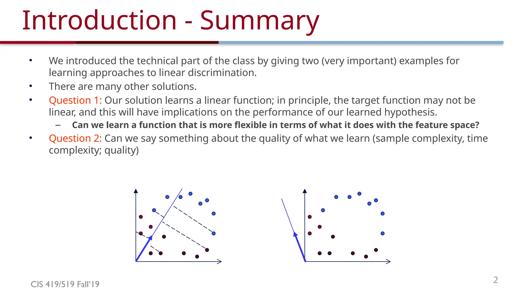
• We introduced the technical part of the class by giving two (very important) examples for
learning approaches to linear discrimination.
• There are many other solutions.
• Question 1: Our solution learns a linear function; in principle, the target function may not be
linear, and this will have implications on the performance of our learned hypothesis.
– Can we learn a function that is more flexible in terms of what it does with the feature space?
• Question 2: Can we say something about the quality of what we learn (sample complexity, time
complexity; quality)

3. CIS 419/519 Fall’19 3
Decision Trees
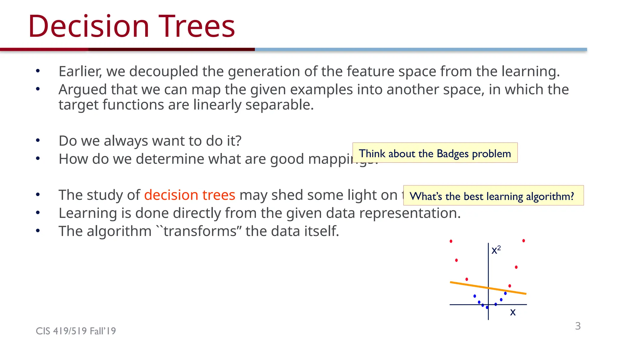
• Earlier, we decoupled the generation of the feature space from the learning.
• Argued that we can map the given examples into another space, in which the
target functions are linearly separable.
• Do we always want to do it?
• How do we determine what are good mappings?
• The study of decision trees may shed some light on this.
• Learning is done directly from the given data representation.
• The algorithm ``transforms” the data itself.
Think about the Badges problem
x
x2
What’s the best learning algorithm?

4. CIS 419/519 Fall’19 4
This Lecture
• Decision trees for (binary) classification
– Non-linear classifiers
• Learning decision trees (ID3 algorithm)
– Greedy heuristic (based on information gain)
Originally developed for discrete features
– Some extensions to the basic algorithm
• Overfitting
– Some experimental issues

5. CIS 419/519 Fall’19
Introduction of Decision trees

6. CIS 419/519 Fall’19 6
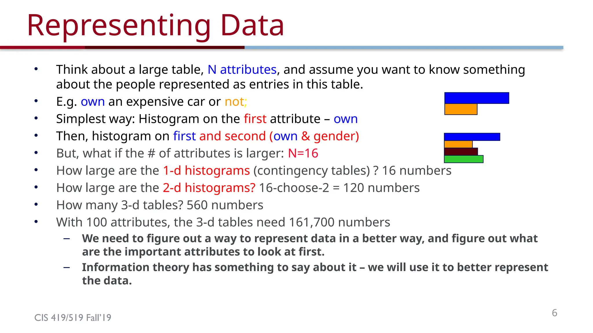
Representing Data
• Think about a large table, N attributes, and assume you want to know something
about the people represented as entries in this table.
• E.g. own an expensive car or not;
• Simplest way: Histogram on the first attribute – own
• Then, histogram on first and second (own & gender)
• But, what if the # of attributes is larger: N=16
• How large are the 1-d histograms (contingency tables) ? 16 numbers
• How large are the 2-d histograms? 16-choose-2 = 120 numbers
• How many 3-d tables? 560 numbers
• With 100 attributes, the 3-d tables need 161,700 numbers
– We need to figure out a way to represent data in a better way, and figure out what
are the important attributes to look at first.
– Information theory has something to say about it – we will use it to better represent
the data.

7. CIS 419/519 Fall’19 7
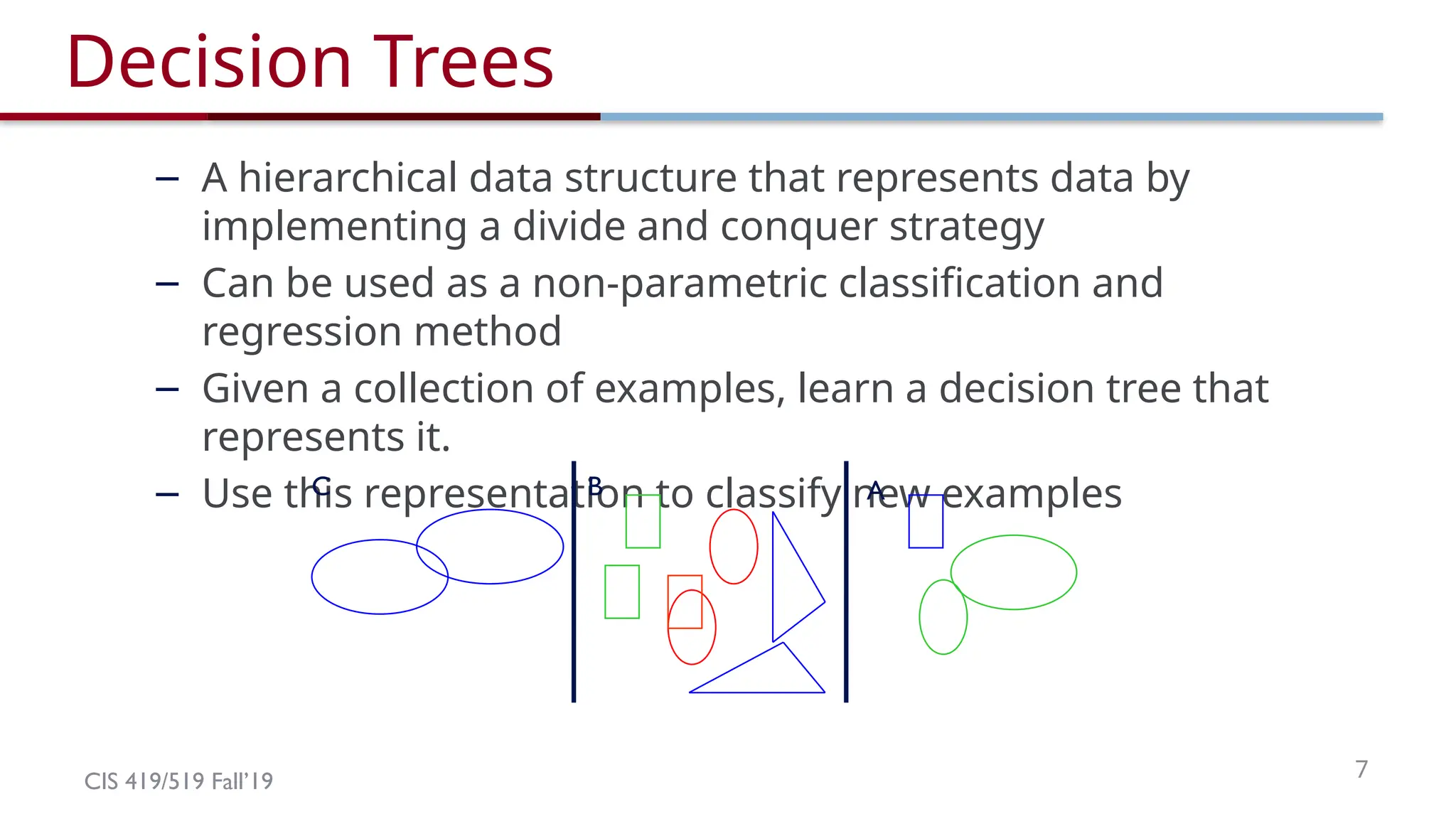
Decision Trees
– A hierarchical data structure that represents data by
implementing a divide and conquer strategy
– Can be used as a non-parametric classification and
regression method
– Given a collection of examples, learn a decision tree that
represents it.
– Use this representation to classify new examples
A
C B

8. CIS 419/519 Fall’19 8
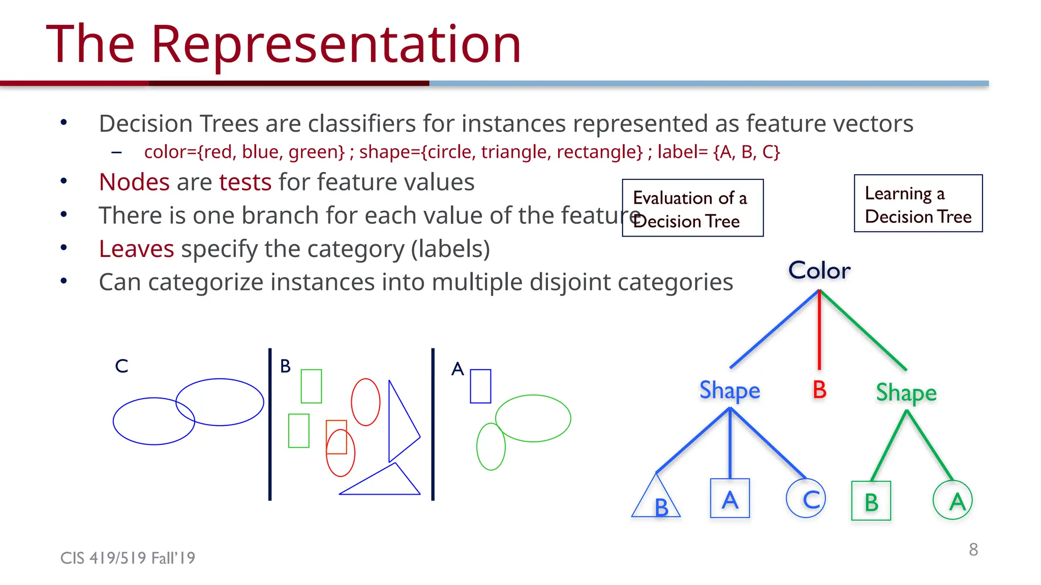
The Representation
• Decision Trees are classifiers for instances represented as feature vectors
– color={red, blue, green} ; shape={circle, triangle, rectangle} ; label= {A, B, C}
• Nodes are tests for feature values
• There is one branch for each value of the feature
• Leaves specify the category (labels)
• Can categorize instances into multiple disjoint categories
Evaluation of a
Decision Tree
Learning a
Decision Tree
Color
Shape Shape
B
A C B A
B
A
C B

9. CIS 419/519 Fall’19 9
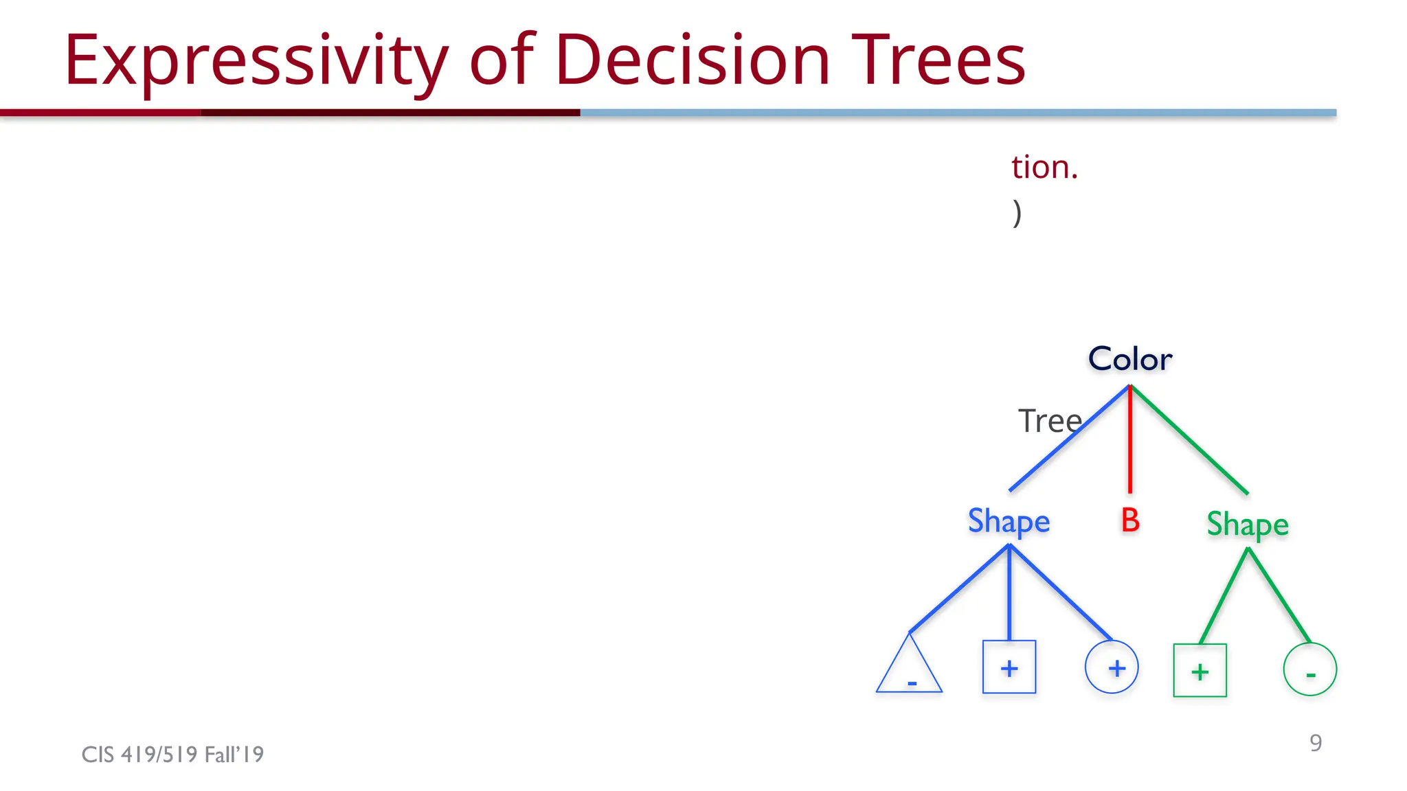
Expressivity of Decision Trees
• As Boolean functions they can represent any Boolean function.
• Can be rewritten as rules in Disjunctive Normal Form (DNF)
– Green ∧ Square  positive
– Blue ∧ Circle  positive
– Blue ∧ Square  positive
• The disjunction of these rules is equivalent to the Decision Tree
• What did we show? What is the hypothesis space here?
– 2 dimensions: color and shape
– 3 values each: color(red, blue, green), shape(triangle, square, circle)
– |X| = 9: (red, triangle), (red, circle), (blue, square) …
– |Y| = 2: + and -
– |H| = 29
Color
Shape Shape
B
+ + + -
-

10. CIS 419/519 Fall’19 10
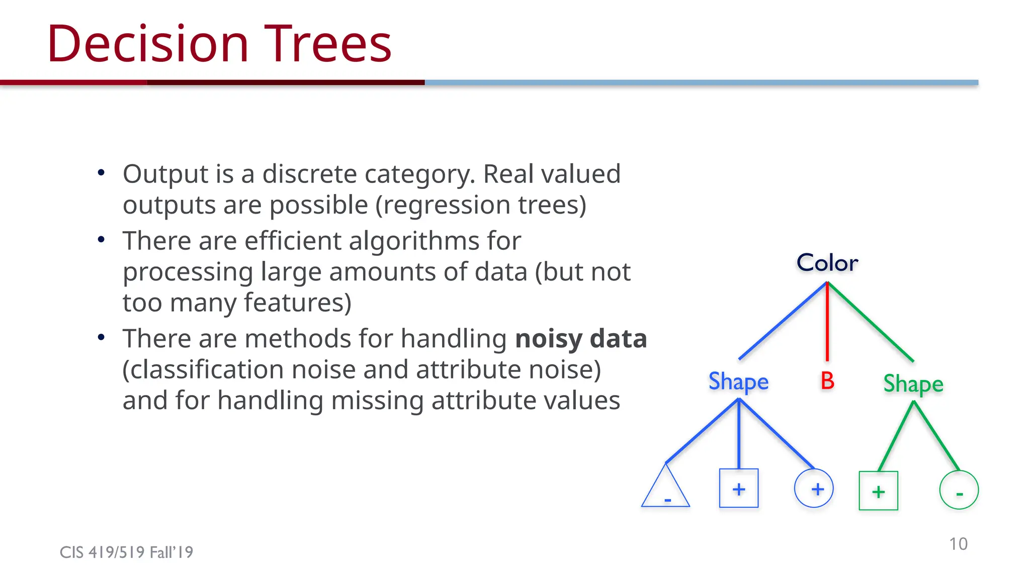
Decision Trees
• Output is a discrete category. Real valued
outputs are possible (regression trees)
• There are efficient algorithms for
processing large amounts of data (but not
too many features)
• There are methods for handling noisy data
(classification noise and attribute noise)
and for handling missing attribute values
Color
Shape Shape
B
+ + + -
-

11. CIS 419/519 Fall’19 11
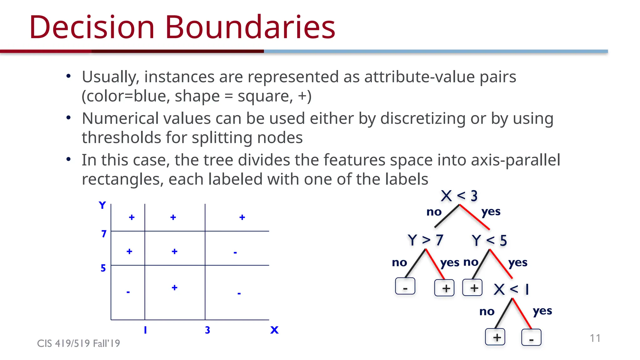
Decision Boundaries
• Usually, instances are represented as attribute-value pairs
(color=blue, shape = square, +)
• Numerical values can be used either by discretizing or by using
thresholds for splitting nodes
• In this case, the tree divides the features space into axis-parallel
rectangles, each labeled with one of the labels
1 3 X
7
5
Y
- +
+ +
+ +
-
-
+
X < 3
Y > 7 Y < 5
X < 1
- + +
+ -
yes
yes
yes
yes
no
no no
no

12. CIS 419/519 Fall’19 12
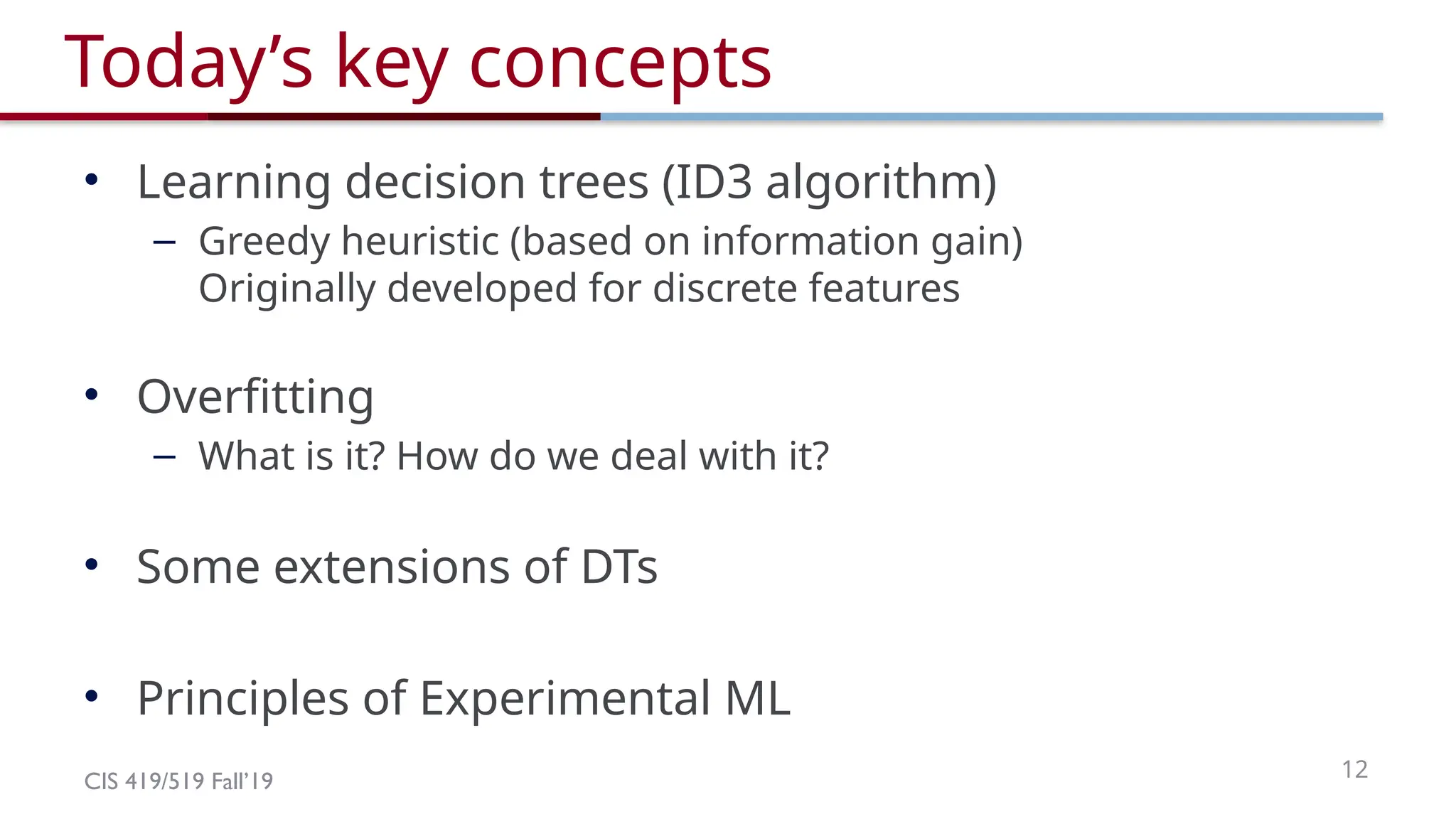
Today’s key concepts
• Learning decision trees (ID3 algorithm)
– Greedy heuristic (based on information gain)
Originally developed for discrete features
• Overfitting
– What is it? How do we deal with it?
• Some extensions of DTs
• Principles of Experimental ML

13. CIS 419/519 Fall’19 13
Administration
• Since there is no waiting list anymore; all people that
wanted to be in are in.
• Everyone should have submitted HW0
• Recitations
• Quizzes
• HW 1 will be released on Monday.
– Please start working on it as soon as you can. Don’t wait until the
last couple of days.
• Questions?
– Please ask/comment during class.

14. CIS 419/519 Fall’19
Learning decision trees (ID3
algorithm

15. CIS 419/519 Fall’19 15
Decision Trees
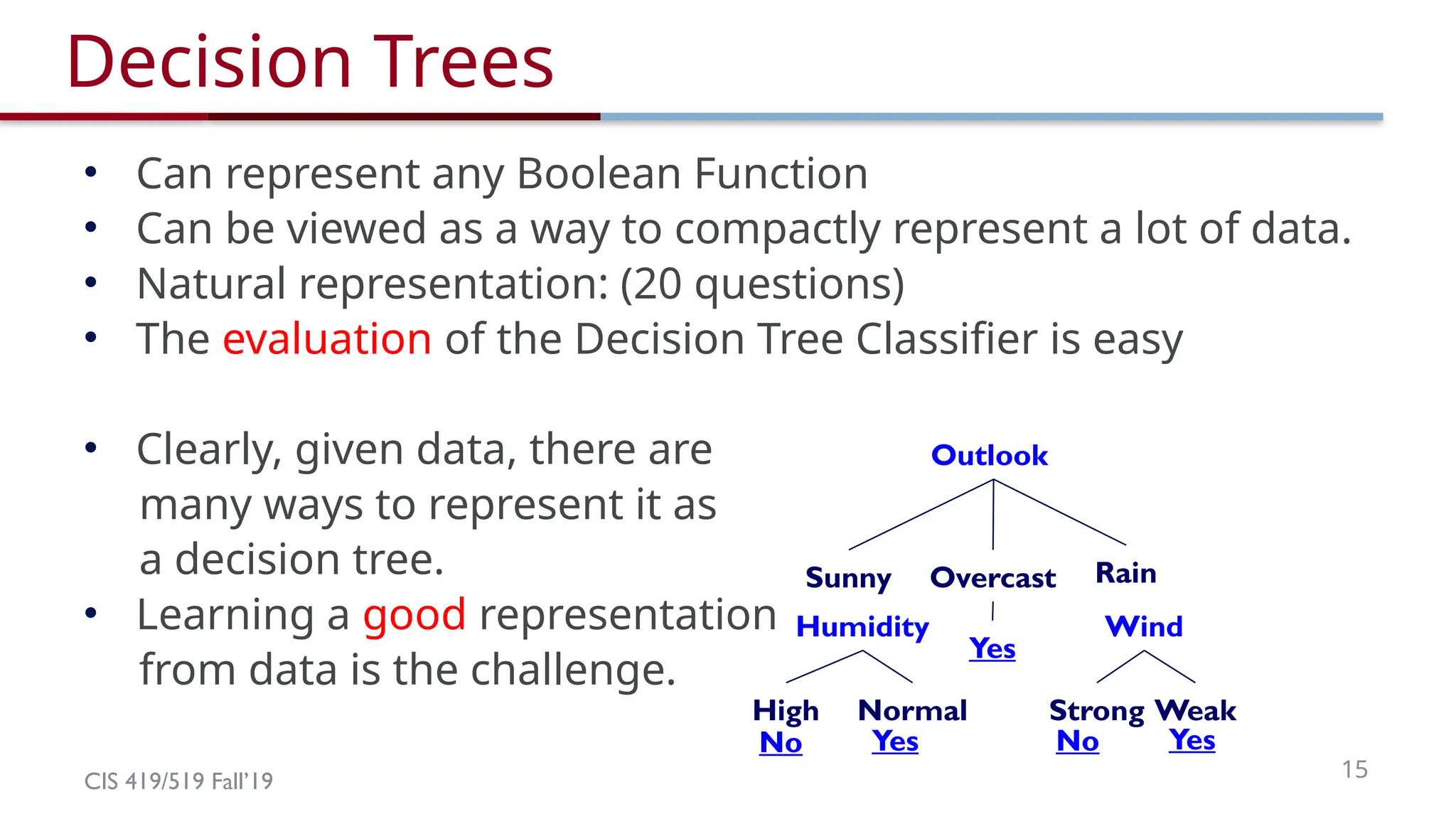
• Can represent any Boolean Function
• Can be viewed as a way to compactly represent a lot of data.
• Natural representation: (20 questions)
• The evaluation of the Decision Tree Classifier is easy
• Clearly, given data, there are
many ways to represent it as
a decision tree.
• Learning a good representation
from data is the challenge.
Yes
Humidity
Normal
High
No Yes
Wind
Weak
Strong
No Yes
Outlook
Overcast Rain
Sunny

16. CIS 419/519 Fall’19 16
Will I play tennis today?
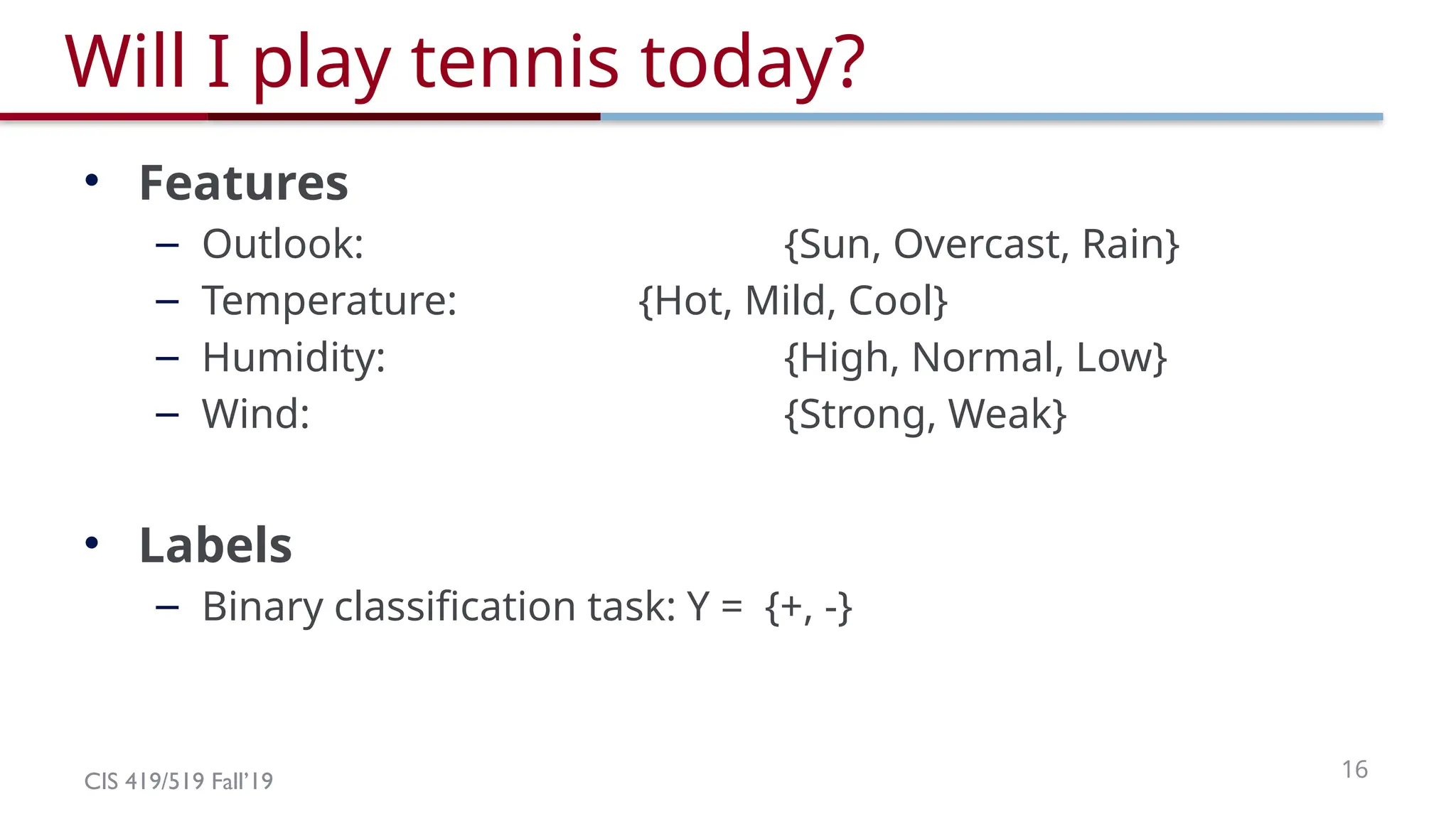
• Features
– Outlook: {Sun, Overcast, Rain}
– Temperature: {Hot, Mild, Cool}
– Humidity: {High, Normal, Low}
– Wind: {Strong, Weak}
• Labels
– Binary classification task: Y = {+, -}

17. CIS 419/519 Fall’19 17
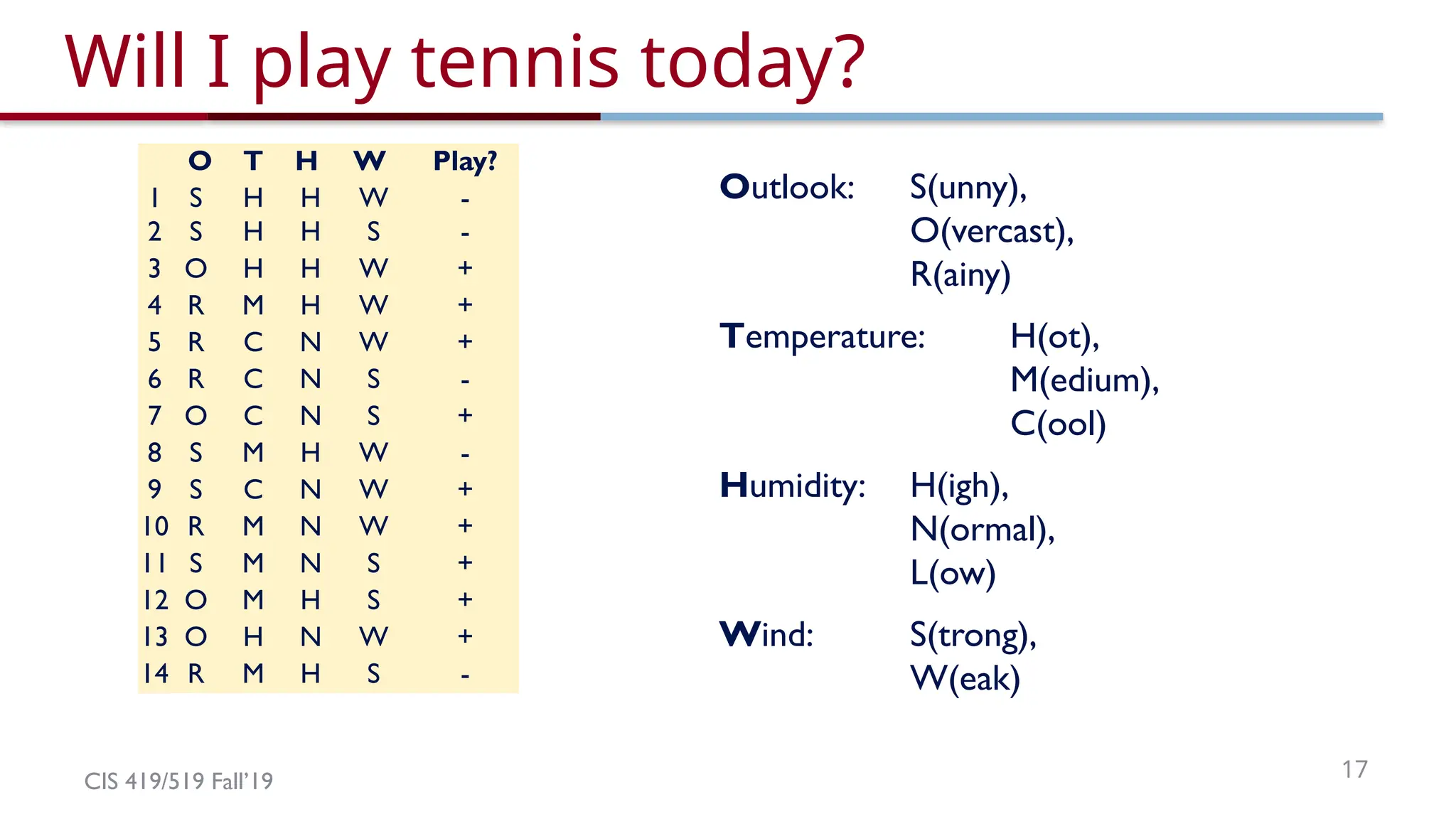
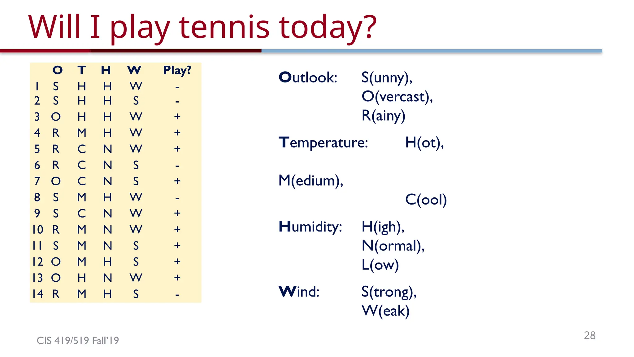
Will I play tennis today?
Outlook: S(unny),
O(vercast),
R(ainy)
Temperature: H(ot),
M(edium),
C(ool)
Humidity: H(igh),
N(ormal),
L(ow)
Wind: S(trong),
W(eak)
O T H W Play?
1 S H H W -
2 S H H S -
3 O H H W +
4 R M H W +
5 R C N W +
6 R C N S -
7 O C N S +
8 S M H W -
9 S C N W +
10 R M N W +
11 S M N S +
12 O M H S +
13 O H N W +
14 R M H S -

18. CIS 419/519 Fall’19
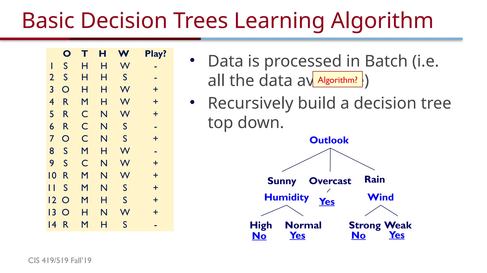
Basic Decision Trees Learning Algorithm
• Data is processed in Batch (i.e.
all the data available)
• Recursively build a decision tree
top down.
Algorithm?
Yes
Humidity
Normal
High
No Yes
Wind
Weak
Strong
No Yes
Outlook
Overcast Rain
Sunny
O T H W Play?
1 S H H W -
2 S H H S -
3 O H H W +
4 R M H W +
5 R C N W +
6 R C N S -
7 O C N S +
8 S M H W -
9 S C N W +
10 R M N W +
11 S M N S +
12 O M H S +
13 O H N W +
14 R M H S -

19. CIS 419/519 Fall’19 19
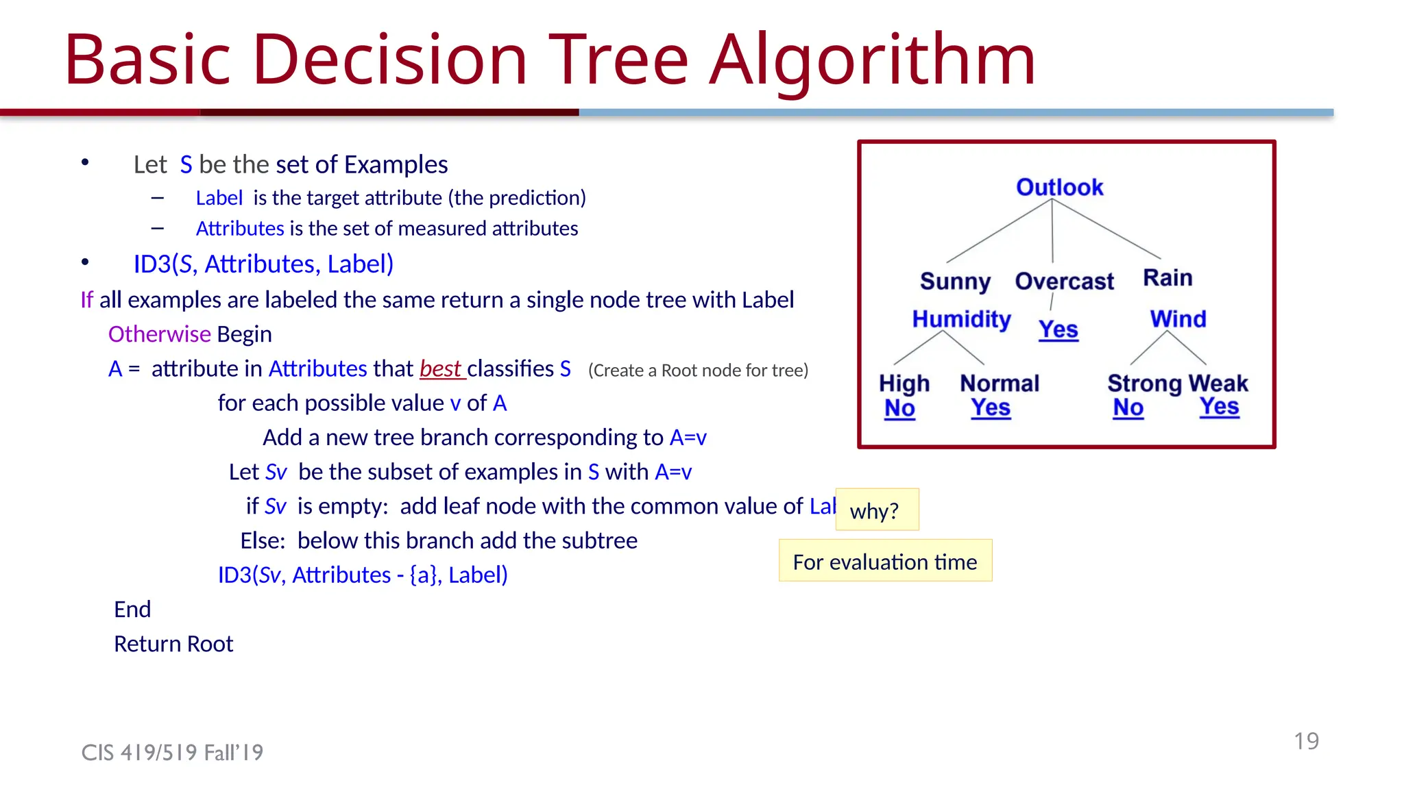
Basic Decision Tree Algorithm
• Let S be the set of Examples
– Label is the target attribute (the prediction)
– Attributes is the set of measured attributes
• ID3(S, Attributes, Label)
If all examples are labeled the same return a single node tree with Label
Otherwise Begin
A = attribute in Attributes that best classifies S (Create a Root node for tree)
for each possible value v of A
Add a new tree branch corresponding to A=v
Let Sv be the subset of examples in S with A=v
if Sv is empty: add leaf node with the common value of Label in S
Else: below this branch add the subtree
ID3(Sv, Attributes - {a}, Label)
End
Return Root
why?
For evaluation time

20. CIS 419/519 Fall’19 20
Picking the Root Attribute
• The goal is to have the resulting decision tree as
small as possible (Occam’s Razor)
– But, finding the minimal decision tree consistent with the
data is NP-hard
• The recursive algorithm is a greedy heuristic search
for a simple tree, but cannot guarantee optimality.
• The main decision in the algorithm is the selection of
the next attribute to condition on.

21. CIS 419/519 Fall’19 21
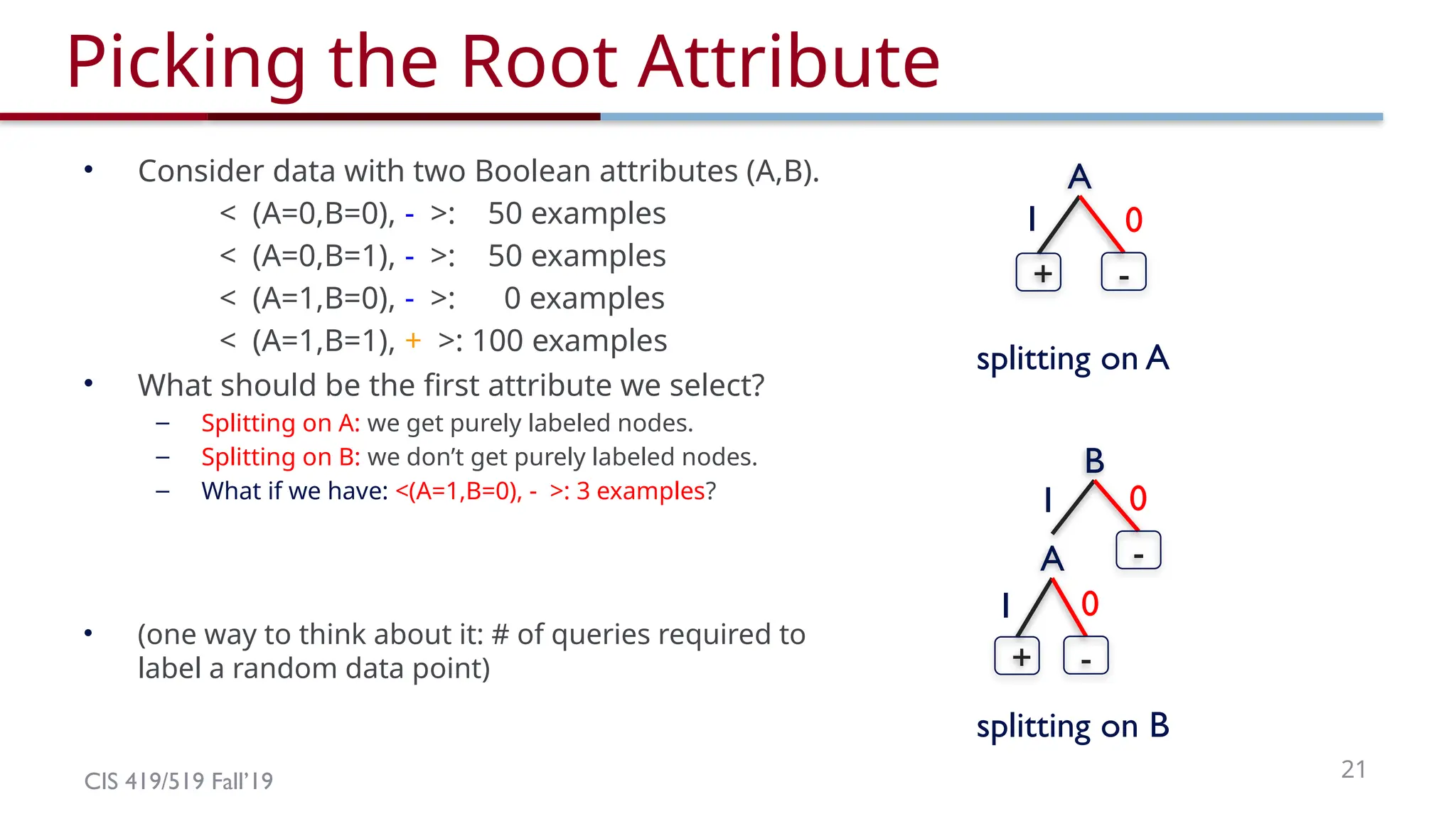
Picking the Root Attribute
• Consider data with two Boolean attributes (A,B).
< (A=0,B=0), - >: 50 examples
< (A=0,B=1), - >: 50 examples
< (A=1,B=0), - >: 0 examples
< (A=1,B=1), + >: 100 examples
• What should be the first attribute we select?
– Splitting on A: we get purely labeled nodes.
– Splitting on B: we don’t get purely labeled nodes.
– What if we have: <(A=1,B=0), - >: 3 examples?
• (one way to think about it: # of queries required to
label a random data point)
A
-
+
1 0
splitting on A
B
-
1 0
A
-
+
1 0
splitting on B

22. CIS 419/519 Fall’19 22
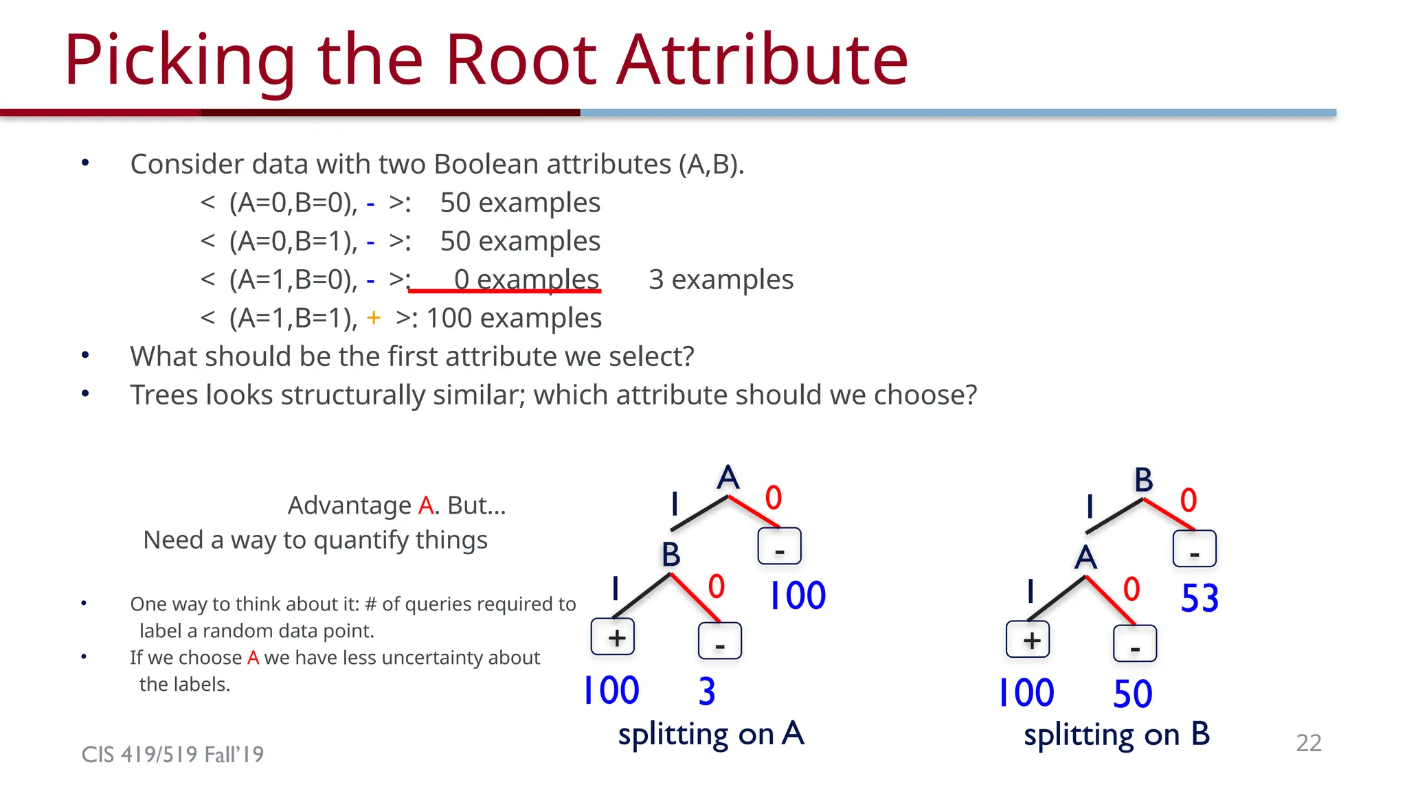
Picking the Root Attribute
• Consider data with two Boolean attributes (A,B).
< (A=0,B=0), - >: 50 examples
< (A=0,B=1), - >: 50 examples
< (A=1,B=0), - >: 0 examples 3 examples
< (A=1,B=1), + >: 100 examples
• What should be the first attribute we select?
• Trees looks structurally similar; which attribute should we choose?
Advantage A. But…
Need a way to quantify things
• One way to think about it: # of queries required to
label a random data point.
• If we choose A we have less uncertainty about
the labels.
53
50
100
B
-
1 0
A
-
+
1 0
100
3
100
A
-
1 0
B
-
+
1 0
splitting on A splitting on B

23. CIS 419/519 Fall’19 23
Picking the Root Attribute
• The goal is to have the resulting decision tree as
small as possible (Occam’s Razor)
– The main decision in the algorithm is the selection of the
next attribute to condition on.
• We want attributes that split the examples to sets
that are relatively pure in one label; this way we are
closer to a leaf node.
– The most popular heuristics is based on information gain,
originated with the ID3 system of Quinlan.

24. CIS 419/519 Fall’19 24
Entropy
• Entropy (impurity, disorder) of a set of examples, S, relative to a binary
classification is:
• is the proportion of positive examples in S and
• is the proportion of negatives examples in S
– If all the examples belong to the same category: Entropy = 0
– If all the examples are equally mixed (0.5, 0.5): Entropy = 1
– Entropy = Level of uncertainty.
• In general, when pi is the fraction of examples labeled i:
• Entropy can be viewed as the number of bits required, on average, to
encode the class of labels. If the probability for + is 0.5, a single bit is
required for each example; if it is 0.8 – can use less then 1 bit.

25. CIS 419/519 Fall’19 25
Entropy
1
-- +
1
-- + --
1
+
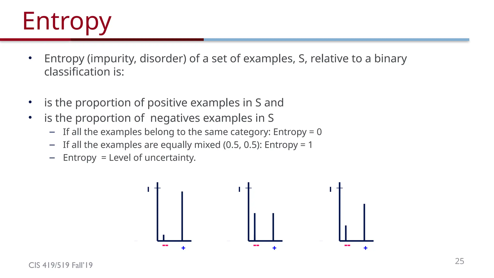
• Entropy (impurity, disorder) of a set of examples, S, relative to a binary
classification is:
• is the proportion of positive examples in S and
• is the proportion of negatives examples in S
– If all the examples belong to the same category: Entropy = 0
– If all the examples are equally mixed (0.5, 0.5): Entropy = 1
– Entropy = Level of uncertainty.

26. CIS 419/519 Fall’19 26
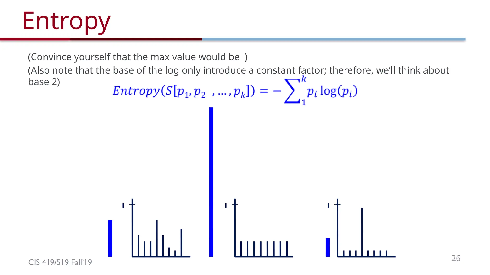
Entropy
1 1 1
(Convince yourself that the max value would be )
(Also note that the base of the log only introduce a constant factor; therefore, we’ll think about
base 2)

27. CIS 419/519 Fall’19 27
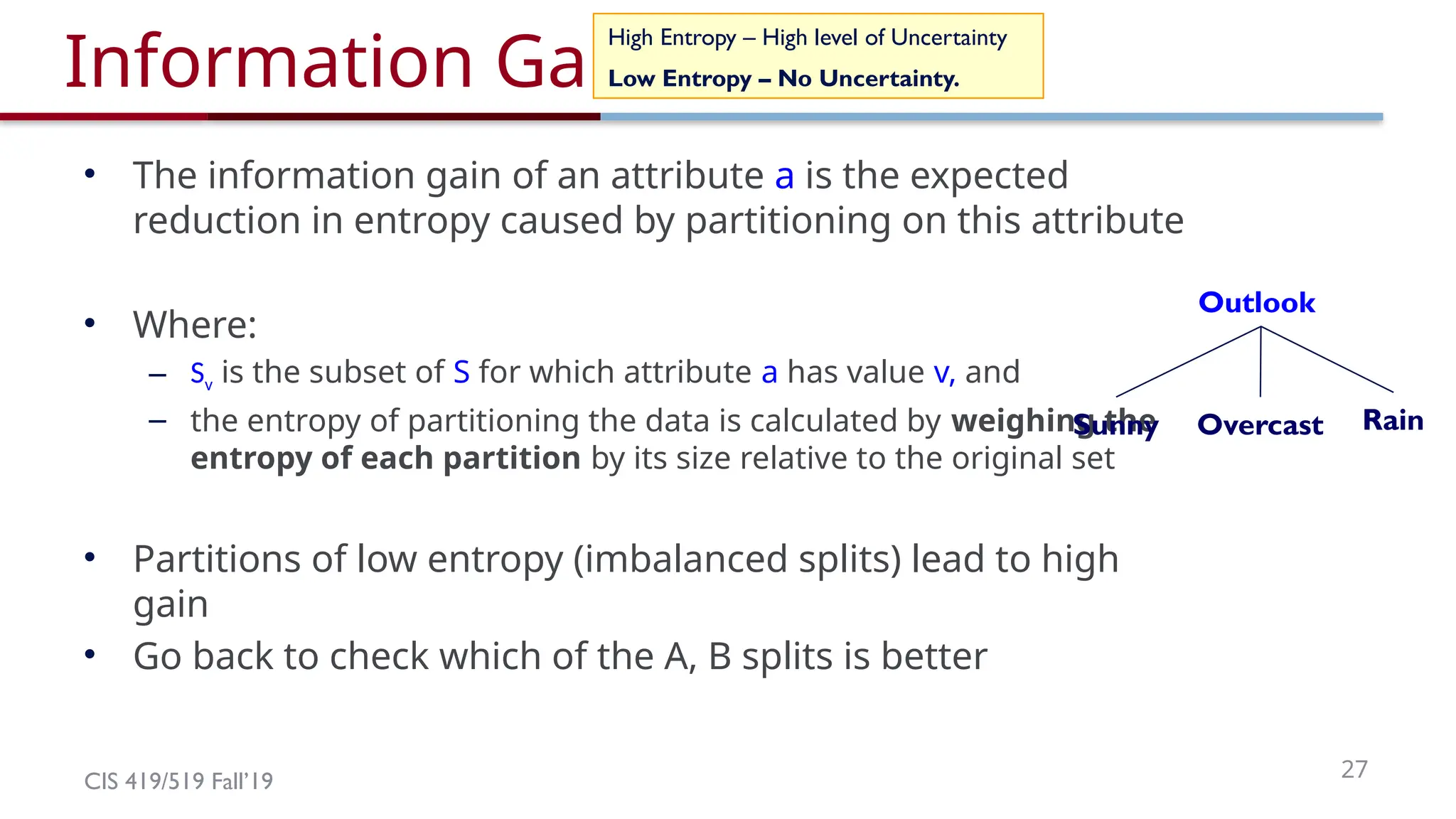
Information Gain
• The information gain of an attribute a is the expected
reduction in entropy caused by partitioning on this attribute
• Where:
– Sv is the subset of S for which attribute a has value v, and
– the entropy of partitioning the data is calculated by weighing the
entropy of each partition by its size relative to the original set
• Partitions of low entropy (imbalanced splits) lead to high
gain
• Go back to check which of the A, B splits is better
High Entropy – High level of Uncertainty
Low Entropy – No Uncertainty.
Outlook
Overcast Rain
Sunny

28. CIS 419/519 Fall’19 28
Will I play tennis today?
O T H W Play?
1 S H H W -
2 S H H S -
3 O H H W +
4 R M H W +
5 R C N W +
6 R C N S -
7 O C N S +
8 S M H W -
9 S C N W +
10 R M N W +
11 S M N S +
12 O M H S +
13 O H N W +
14 R M H S -
Outlook: S(unny),
O(vercast),
R(ainy)
Temperature: H(ot),
M(edium),
C(ool)
Humidity: H(igh),
N(ormal),
L(ow)
Wind: S(trong),
W(eak)

29. CIS 419/519 Fall’19 29
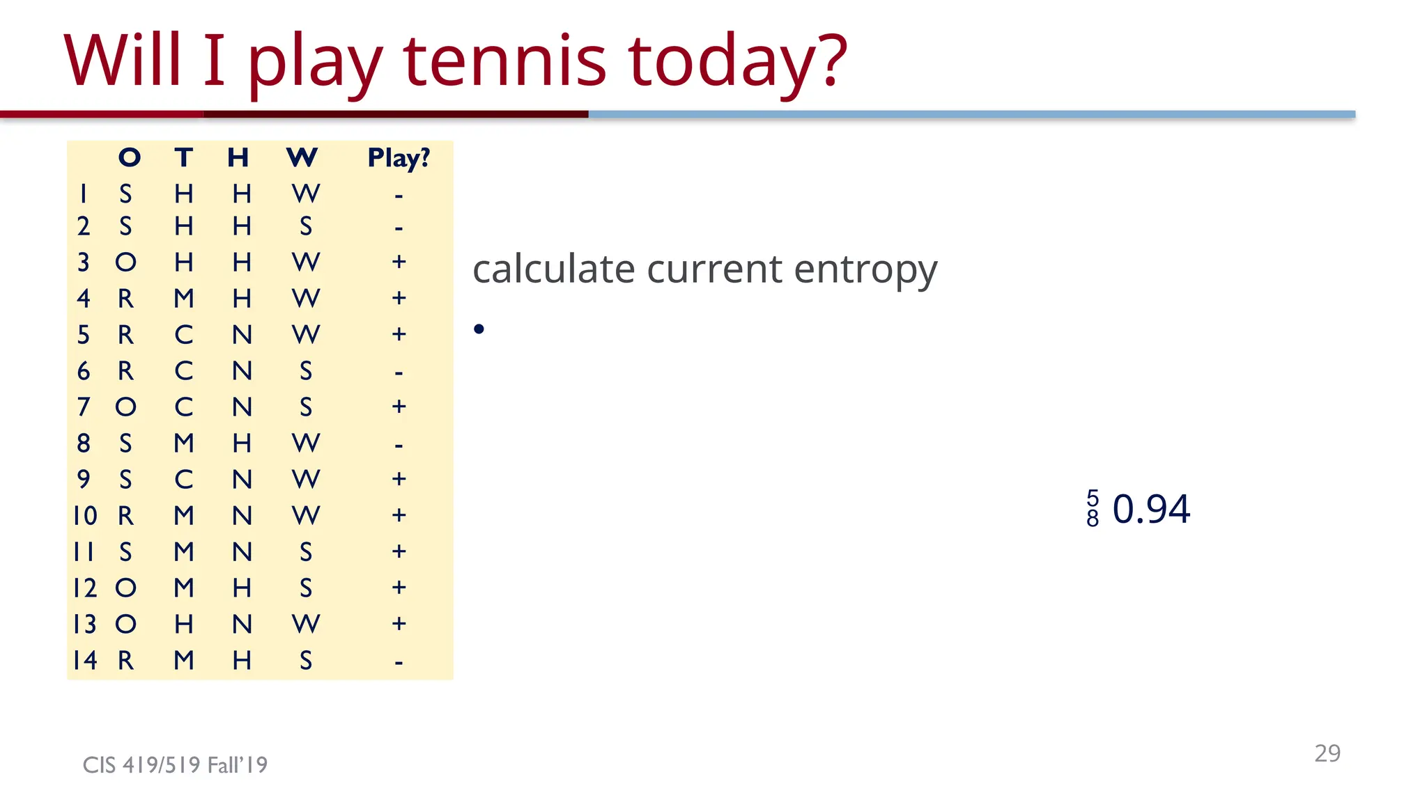
Will I play tennis today?
O T H W Play?
1 S H H W -
2 S H H S -
3 O H H W +
4 R M H W +
5 R C N W +
6 R C N S -
7 O C N S +
8 S M H W -
9 S C N W +
10 R M N W +
11 S M N S +
12 O M H S +
13 O H N W +
14 R M H S -
calculate current entropy
•
 0.94

30. CIS 419/519 Fall’19 30
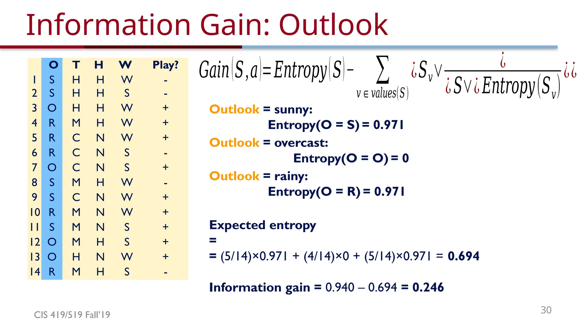
Information Gain: Outlook
O T H W Play?
1 S H H W -
2 S H H S -
3 O H H W +
4 R M H W +
5 R C N W +
6 R C N S -
7 O C N S +
8 S M H W -
9 S C N W +
10 R M N W +
11 S M N S +
12 O M H S +
13 O H N W +
14 R M H S -
Outlook = sunny:
Entropy(O = S) = 0.971
Outlook = overcast:
Entropy(O = O) = 0
Outlook = rainy:
Entropy(O = R) = 0.971
Expected entropy
=
= (5/14)×0.971 + (4/14)×0 + (5/14)×0.971 = 0.694
Information gain = 0.940 – 0.694 = 0.246
𝐺𝑎𝑖𝑛(𝑆,𝑎)=𝐸𝑛𝑡𝑟𝑜𝑝𝑦(𝑆)− ∑
𝑣∈𝑣𝑎𝑙𝑢𝑒𝑠(𝑆)
¿𝑆𝑣∨ ¿
¿𝑆∨¿𝐸𝑛𝑡𝑟𝑜𝑝𝑦(𝑆𝑣)
¿¿

31. CIS 419/519 Fall’19 31
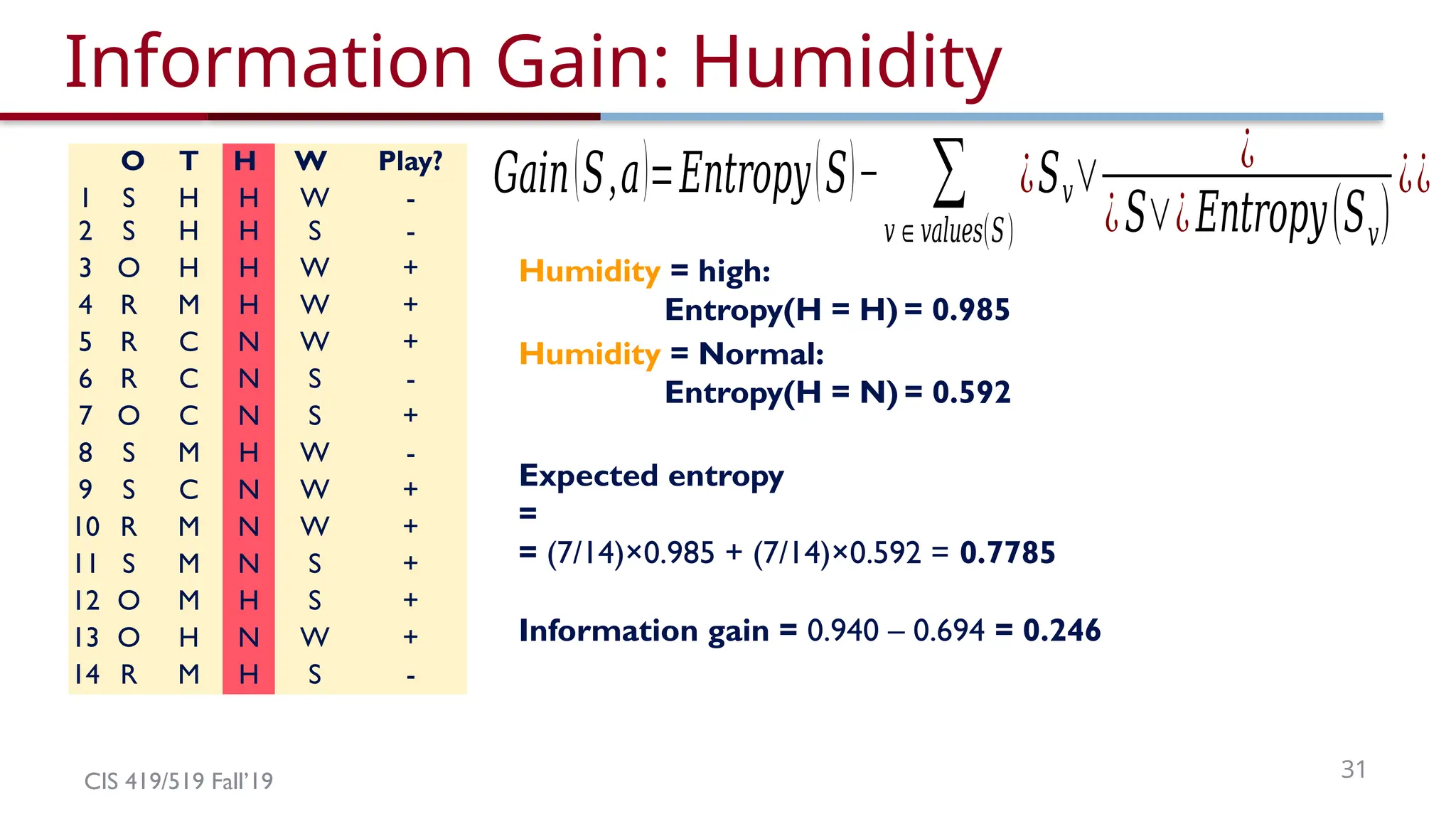
Information Gain: Humidity
O T H W Play?
1 S H H W -
2 S H H S -
3 O H H W +
4 R M H W +
5 R C N W +
6 R C N S -
7 O C N S +
8 S M H W -
9 S C N W +
10 R M N W +
11 S M N S +
12 O M H S +
13 O H N W +
14 R M H S -
Humidity = high:
Entropy(H = H) = 0.985
Humidity = Normal:
Entropy(H = N) = 0.592
Expected entropy
=
= (7/14)×0.985 + (7/14)×0.592 = 0.7785
Information gain = 0.940 – 0.694 = 0.246
𝐺𝑎𝑖𝑛(𝑆,𝑎)=𝐸𝑛𝑡𝑟𝑜𝑝𝑦(𝑆)− ∑
𝑣∈𝑣𝑎𝑙𝑢𝑒𝑠(𝑆)
¿𝑆𝑣∨ ¿
¿𝑆∨¿𝐸𝑛𝑡𝑟𝑜𝑝𝑦(𝑆𝑣)
¿¿

32. CIS 419/519 Fall’19 32
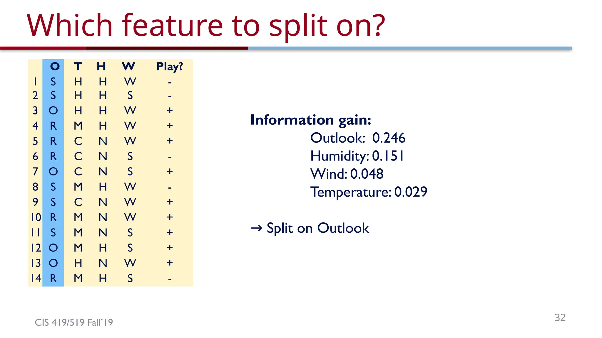
Which feature to split on?
O T H W Play?
1 S H H W -
2 S H H S -
3 O H H W +
4 R M H W +
5 R C N W +
6 R C N S -
7 O C N S +
8 S M H W -
9 S C N W +
10 R M N W +
11 S M N S +
12 O M H S +
13 O H N W +
14 R M H S -
Information gain:
Outlook: 0.246
Humidity: 0.151
Wind: 0.048
Temperature: 0.029
→ Split on Outlook

33. CIS 419/519 Fall’19 33
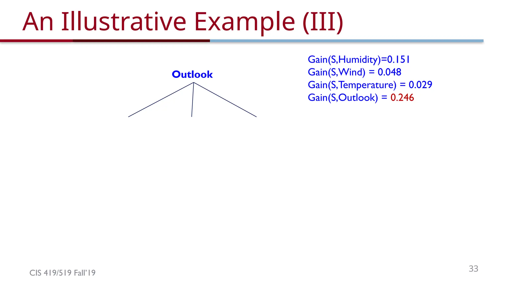
An Illustrative Example (III)
Outlook
Gain(S,Humidity)=0.151
Gain(S,Wind) = 0.048
Gain(S,Temperature) = 0.029
Gain(S,Outlook) = 0.246

34. CIS 419/519 Fall’19 34
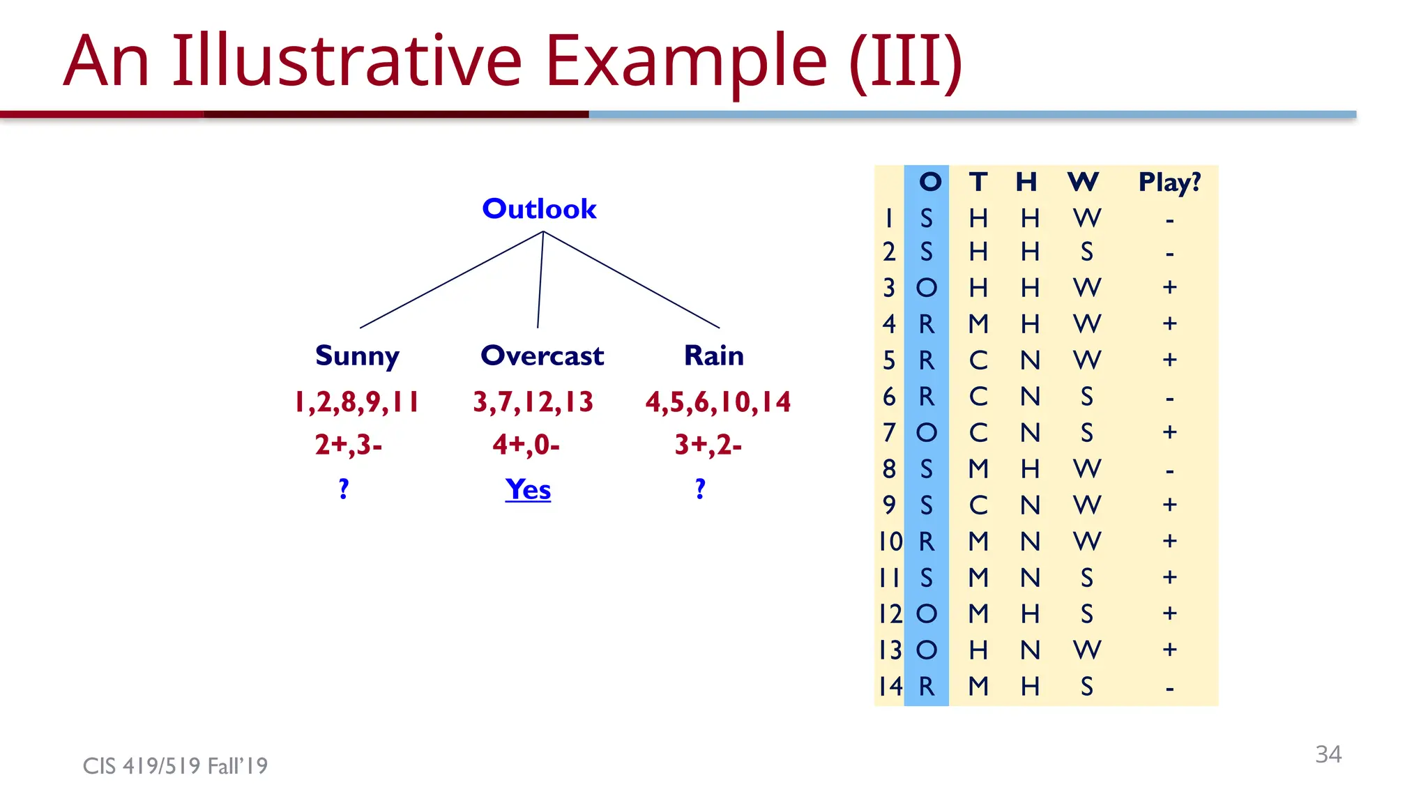
An Illustrative Example (III)
Outlook
Overcast Rain
3,7,12,13 4,5,6,10,14
3+,2-
Sunny
1,2,8,9,11
4+,0-
2+,3-
Yes
? ?
O T H W Play?
1 S H H W -
2 S H H S -
3 O H H W +
4 R M H W +
5 R C N W +
6 R C N S -
7 O C N S +
8 S M H W -
9 S C N W +
10 R M N W +
11 S M N S +
12 O M H S +
13 O H N W +
14 R M H S -

35. CIS 419/519 Fall’19 35
An Illustrative Example (III)
Outlook
Overcast Rain
3,7,12,13 4,5,6,10,14
3+,2-
Sunny
1,2,8,9,11
4+,0-
2+,3-
Yes
? ?
Continue until:
• Every attribute is included in path, or,
• All examples in the leaf have same label
O T H W Play?
1 S H H W -
2 S H H S -
3 O H H W +
4 R M H W +
5 R C N W +
6 R C N S -
7 O C N S +
8 S M H W -
9 S C N W +
10 R M N W +
11 S M N S +
12 O M H S +
13 O H N W +
14 R M H S -

36. CIS 419/519 Fall’19 36
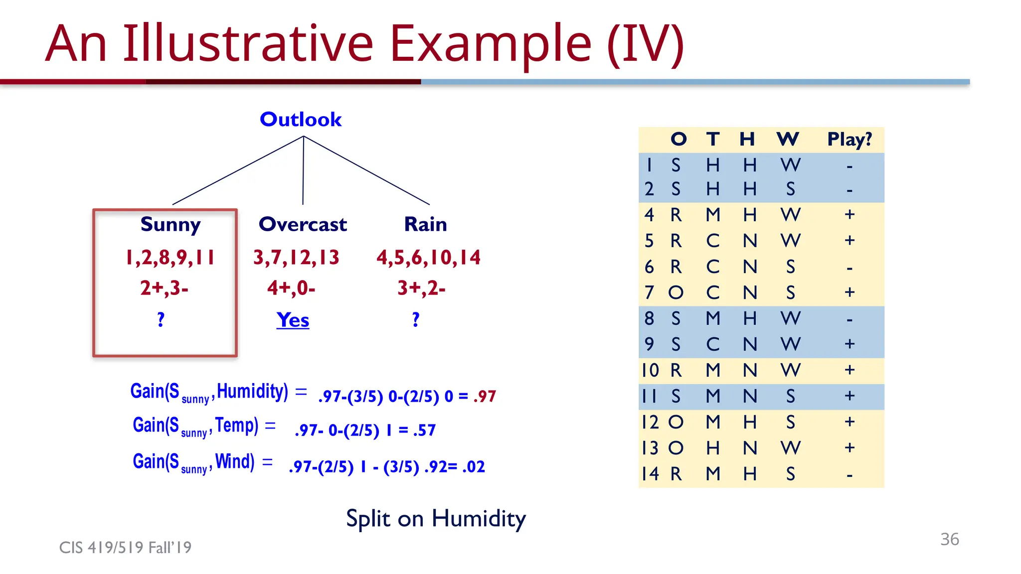
An Illustrative Example (IV)

Humidity)
,
Gain(Ssunny .97-(3/5) 0-(2/5) 0 = .97

Temp)
,
Gain(Ssunny .97- 0-(2/5) 1 = .57

Wind)
,
Gain(Ssunny .97-(2/5) 1 - (3/5) .92= .02
Outlook
Overcast Rain
3,7,12,13 4,5,6,10,14
3+,2-
Sunny
1,2,8,9,11
4+,0-
2+,3-
Yes
? ?
O T H W Play?
1 S H H W -
2 S H H S -
4 R M H W +
5 R C N W +
6 R C N S -
7 O C N S +
8 S M H W -
9 S C N W +
10 R M N W +
11 S M N S +
12 O M H S +
13 O H N W +
14 R M H S -
Split on Humidity

37. CIS 419/519 Fall’19 37
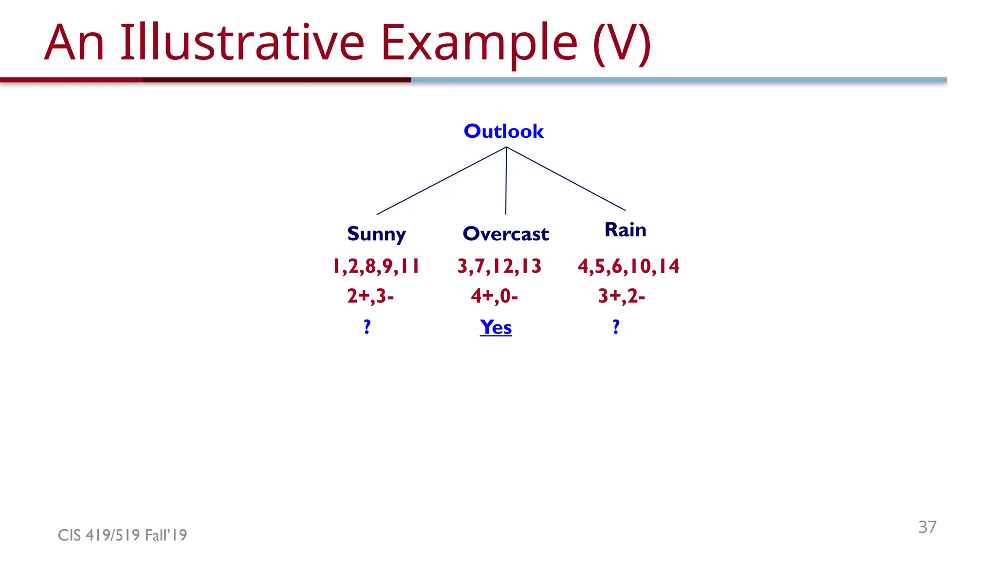
An Illustrative Example (V)
Outlook
Overcast Rain
3,7,12,13 4,5,6,10,14
3+,2-
Sunny
1,2,8,9,11
4+,0-
2+,3-
Yes
? ?

38. CIS 419/519 Fall’19 38
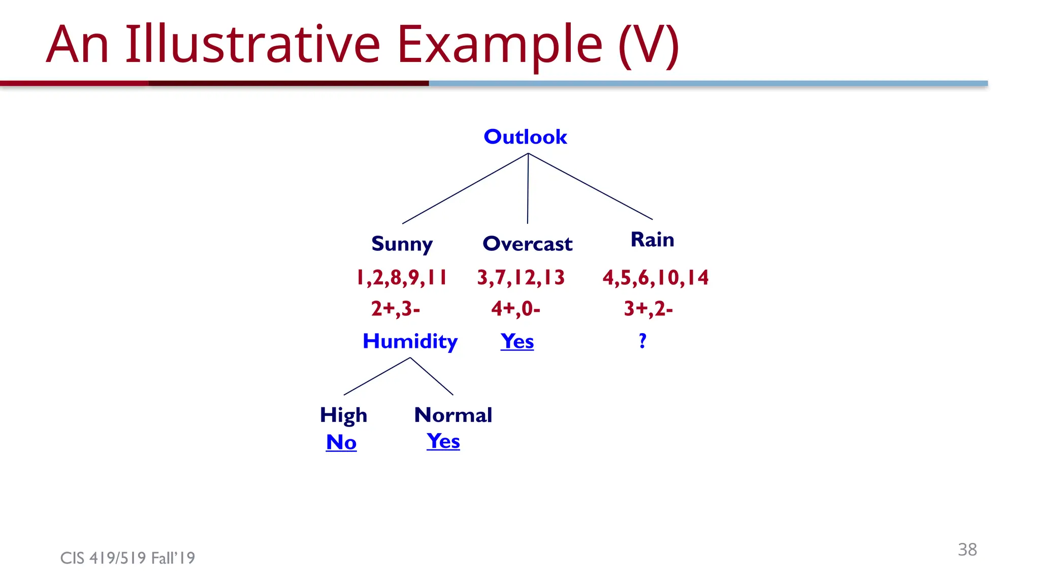
An Illustrative Example (V)
Outlook
Overcast Rain
3,7,12,13 4,5,6,10,14
3+,2-
Sunny
1,2,8,9,11
4+,0-
2+,3-
Yes
Humidity ?
Normal
High
No Yes

39. CIS 419/519 Fall’19 39
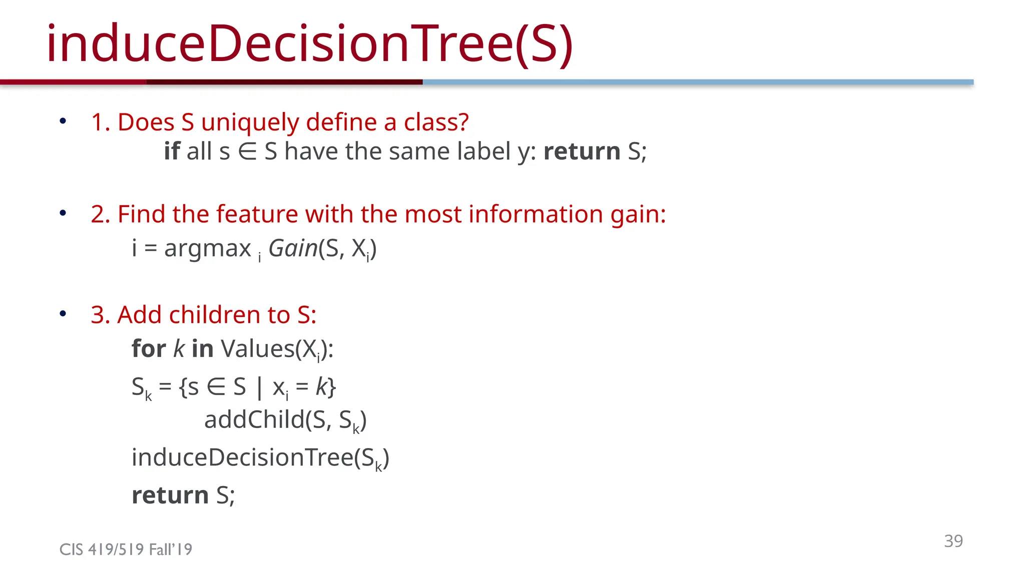
induceDecisionTree(S)
• 1. Does S uniquely define a class?
if all s S have the same label y:
∈ return S;
• 2. Find the feature with the most information gain:
i = argmax i Gain(S, Xi)
• 3. Add children to S:
for k in Values(Xi):
Sk = {s S | x
∈ i = k}
addChild(S, Sk)
induceDecisionTree(Sk)
return S;

40. CIS 419/519 Fall’19 40
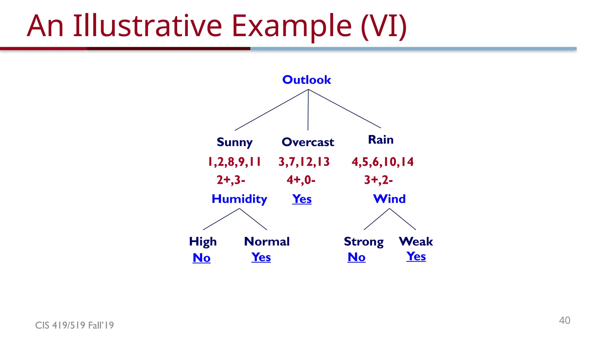
An Illustrative Example (VI)
Outlook
Overcast Rain
3,7,12,13 4,5,6,10,14
3+,2-
Sunny
1,2,8,9,11
4+,0-
2+,3-
Yes
Humidity Wind
Normal
High
No Yes
Weak
Strong
No Yes

41. CIS 419/519 Fall’19 41
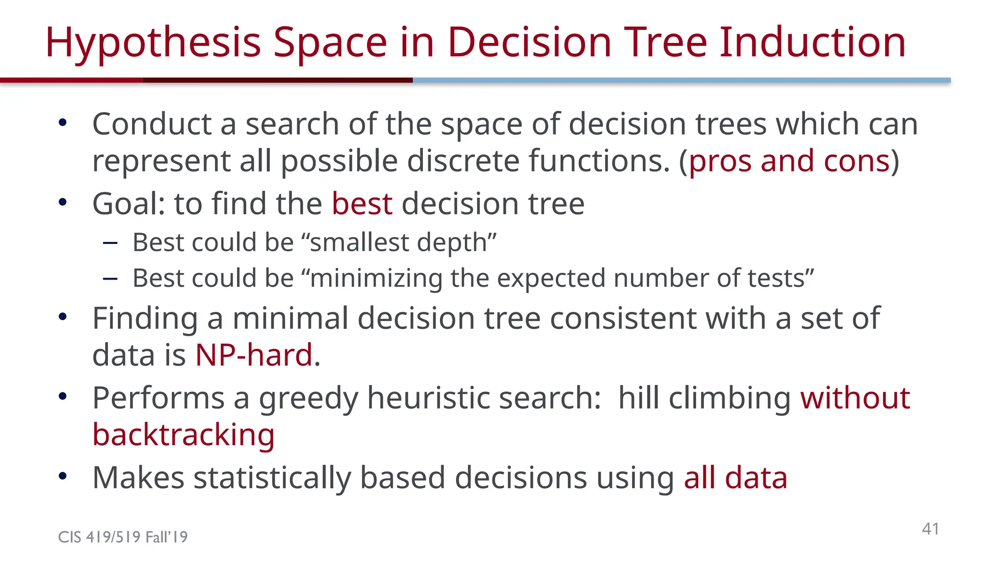
Hypothesis Space in Decision Tree Induction
• Conduct a search of the space of decision trees which can
represent all possible discrete functions. (pros and cons)
• Goal: to find the best decision tree
– Best could be “smallest depth”
– Best could be “minimizing the expected number of tests”
• Finding a minimal decision tree consistent with a set of
data is NP-hard.
• Performs a greedy heuristic search: hill climbing without
backtracking
• Makes statistically based decisions using all data

42. CIS 419/519 Fall’19 42
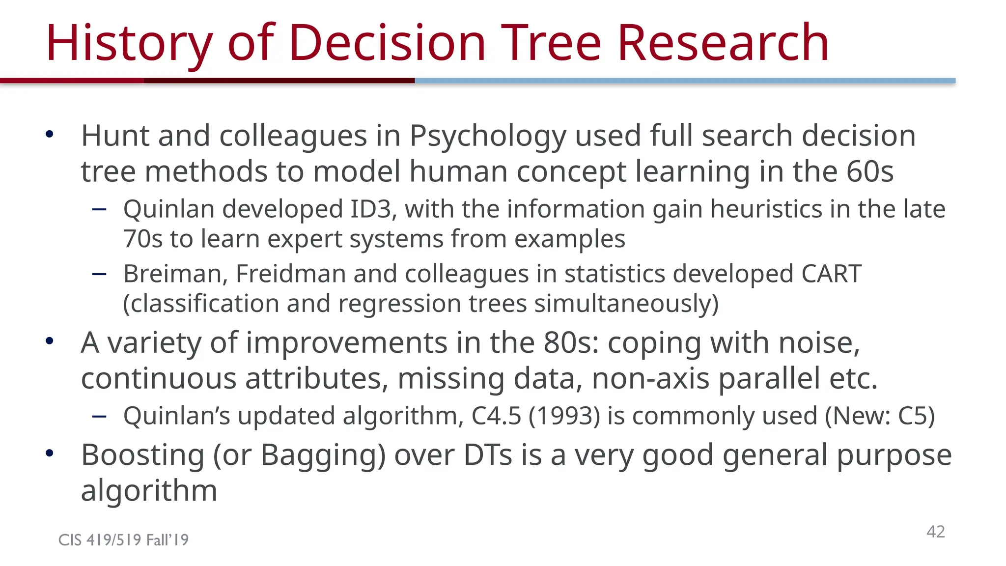
History of Decision Tree Research
• Hunt and colleagues in Psychology used full search decision
tree methods to model human concept learning in the 60s
– Quinlan developed ID3, with the information gain heuristics in the late
70s to learn expert systems from examples
– Breiman, Freidman and colleagues in statistics developed CART
(classification and regression trees simultaneously)
• A variety of improvements in the 80s: coping with noise,
continuous attributes, missing data, non-axis parallel etc.
– Quinlan’s updated algorithm, C4.5 (1993) is commonly used (New: C5)
• Boosting (or Bagging) over DTs is a very good general purpose
algorithm

43. CIS 419/519 Fall’19
Overfitting

44. CIS 419/519 Fall’19 44
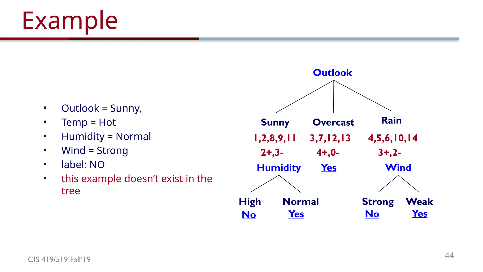
Example
Outlook
Overcast Rain
3,7,12,13 4,5,6,10,14
3+,2-
Sunny
1,2,8,9,11
4+,0-
2+,3-
Yes
Humidity Wind
Normal
High
No Yes
Weak
Strong
No Yes
• Outlook = Sunny,
• Temp = Hot
• Humidity = Normal
• Wind = Strong
• label: NO
• this example doesn’t exist in the
tree

45. CIS 419/519 Fall’19 45
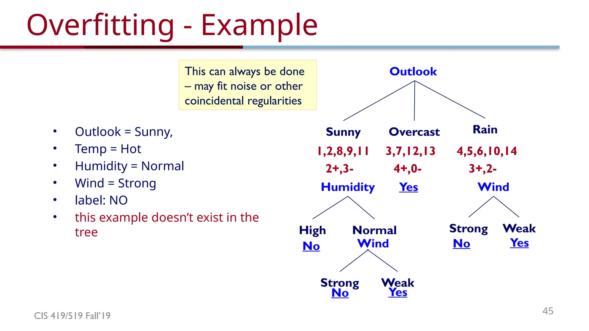
Overfitting - Example
Outlook
Overcast Rain
3,7,12,13 4,5,6,10,14
3+,2-
Sunny
1,2,8,9,11
4+,0-
2+,3-
Yes
Humidity Wind
Normal
High
No
Weak
Strong
No Yes
Weak
Strong
No Yes
Wind
This can always be done
– may fit noise or other
coincidental regularities
• Outlook = Sunny,
• Temp = Hot
• Humidity = Normal
• Wind = Strong
• label: NO
• this example doesn’t exist in the
tree

46. CIS 419/519 Fall’19 46
Our training data

47. CIS 419/519 Fall’19 47
The instance space

48. CIS 419/519 Fall’19 48
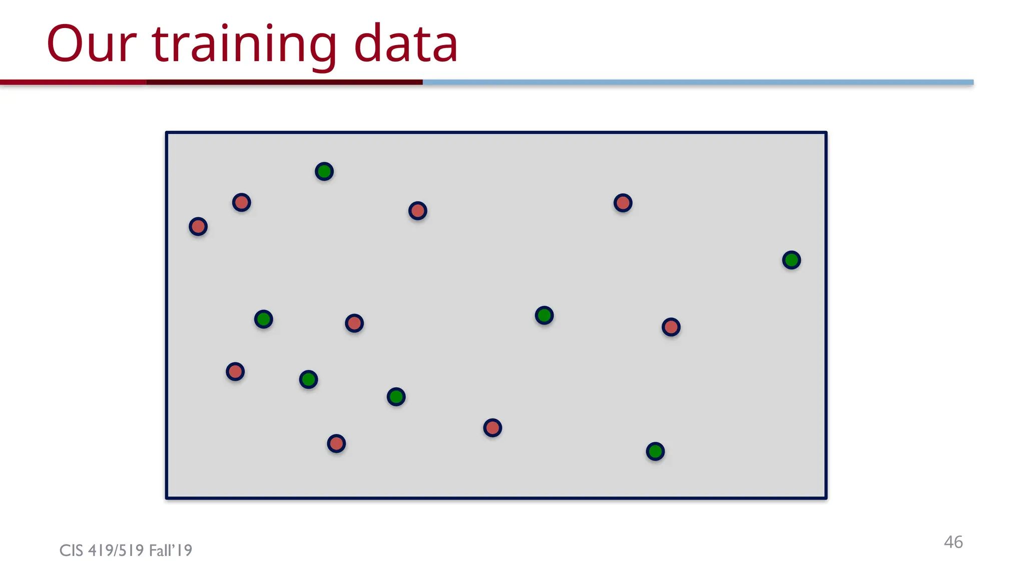
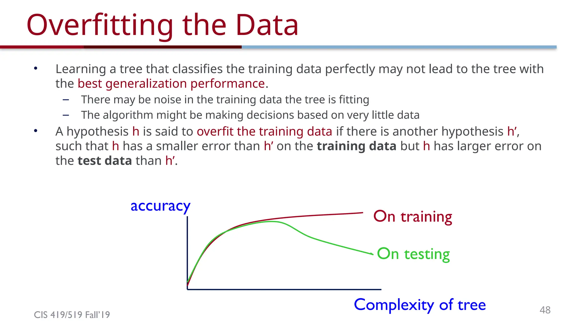
Overfitting the Data
• Learning a tree that classifies the training data perfectly may not lead to the tree with
the best generalization performance.
– There may be noise in the training data the tree is fitting
– The algorithm might be making decisions based on very little data
• A hypothesis h is said to overfit the training data if there is another hypothesis h’,
such that h has a smaller error than h’ on the training data but h has larger error on
the test data than h’.
Complexity of tree
accuracy
On testing
On training

49. CIS 419/519 Fall’19 49
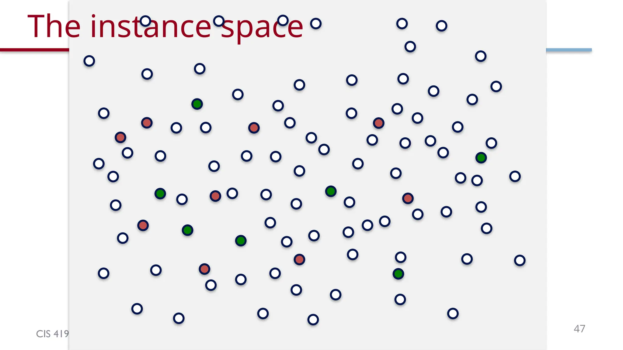
Reasons for overfitting
• Too much variance in the training data
– Training data is not a representative sample
of the instance space
– We split on features that are actually irrelevant
• Too much noise in the training data
– Noise = some feature values or class labels are incorrect
– We learn to predict the noise
• In both cases, it is a result of our will to minimize the empirical
error when we learn, and the ability to do it (with DTs)

50. CIS 419/519 Fall’19 50
Pruning a decision tree
• Prune = remove leaves and assign majority label of
the parent to all items
• Prune the children of node s if:
– all children are leaves, and
– the accuracy on the validation set does not decrease if we
assign the most frequent class label to all items at s.

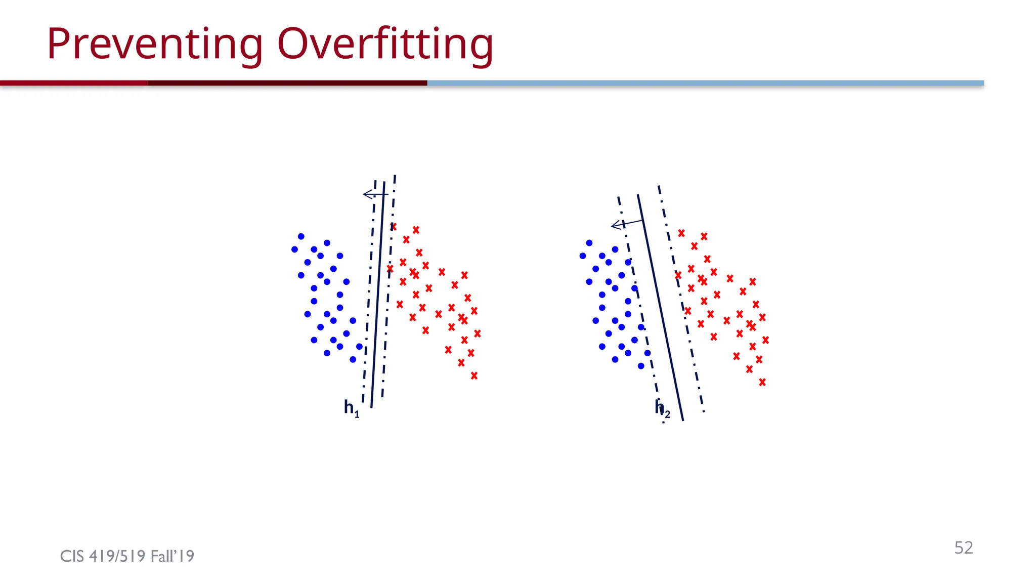
51. CIS 419/519 Fall’19 51
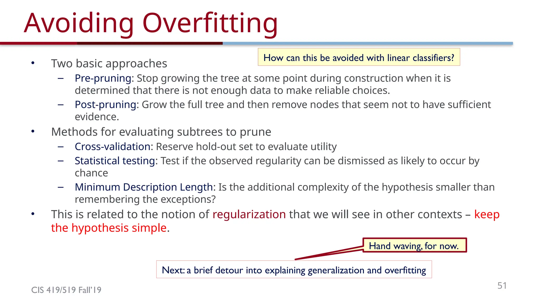
Avoiding Overfitting
• Two basic approaches
– Pre-pruning: Stop growing the tree at some point during construction when it is
determined that there is not enough data to make reliable choices.
– Post-pruning: Grow the full tree and then remove nodes that seem not to have sufficient
evidence.
• Methods for evaluating subtrees to prune
– Cross-validation: Reserve hold-out set to evaluate utility
– Statistical testing: Test if the observed regularity can be dismissed as likely to occur by
chance
– Minimum Description Length: Is the additional complexity of the hypothesis smaller than
remembering the exceptions?
• This is related to the notion of regularization that we will see in other contexts – keep
the hypothesis simple.
How can this be avoided with linear classifiers?
Next: a brief detour into explaining generalization and overfitting
Hand waving, for now.

52. CIS 419/519 Fall’19 52
Preventing Overfitting
h1 h2

53. CIS 419/519 Fall’19 56
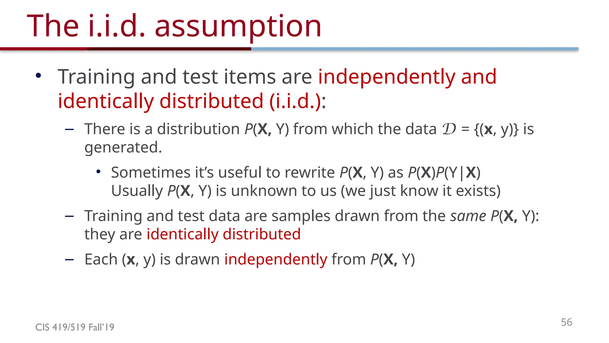
The i.i.d. assumption
• Training and test items are independently and
identically distributed (i.i.d.):
– There is a distribution P(X, Y) from which the data D = {(x, y)} is
generated.
• Sometimes it’s useful to rewrite P(X, Y) as P(X)P(Y|X)
Usually P(X, Y) is unknown to us (we just know it exists)
– Training and test data are samples drawn from the same P(X, Y):
they are identically distributed
– Each (x, y) is drawn independently from P(X, Y)

54. CIS 419/519 Fall’19 57
Size of tree
Accuracy
On test data
On training data
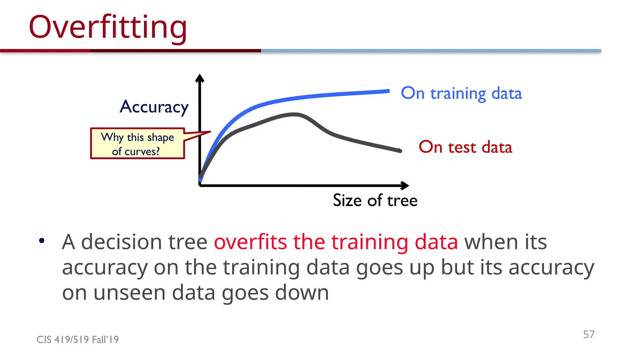
Overfitting
• A decision tree overfits the training data when its
accuracy on the training data goes up but its accuracy
on unseen data goes down
Why this shape
of curves?

55. CIS 419/519 Fall’19 58
Model complexity
Empirical
Error
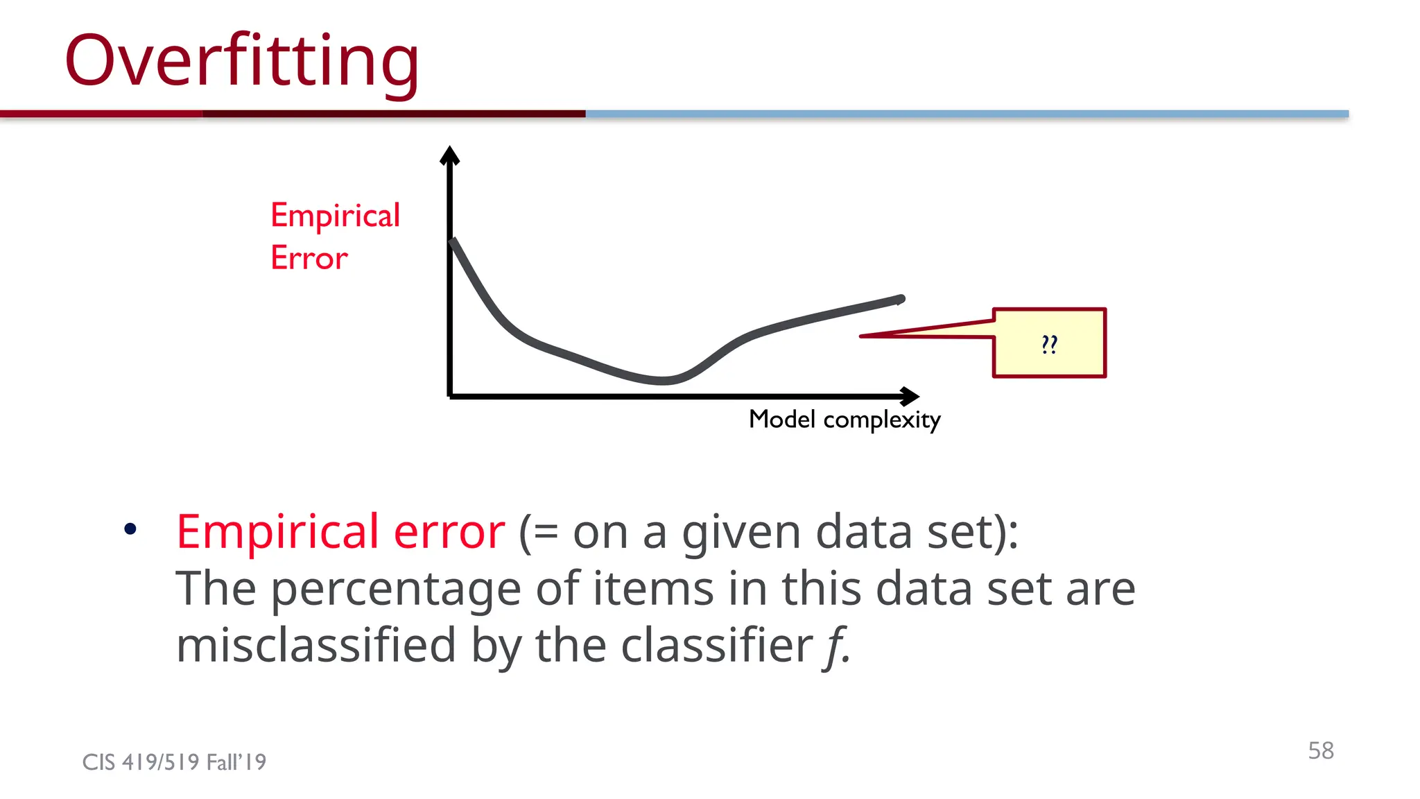
Overfitting
• Empirical error (= on a given data set):
The percentage of items in this data set are
misclassified by the classifier f.
??

56. CIS 419/519 Fall’19 59
Model complexity
Empirical
Error
Overfitting
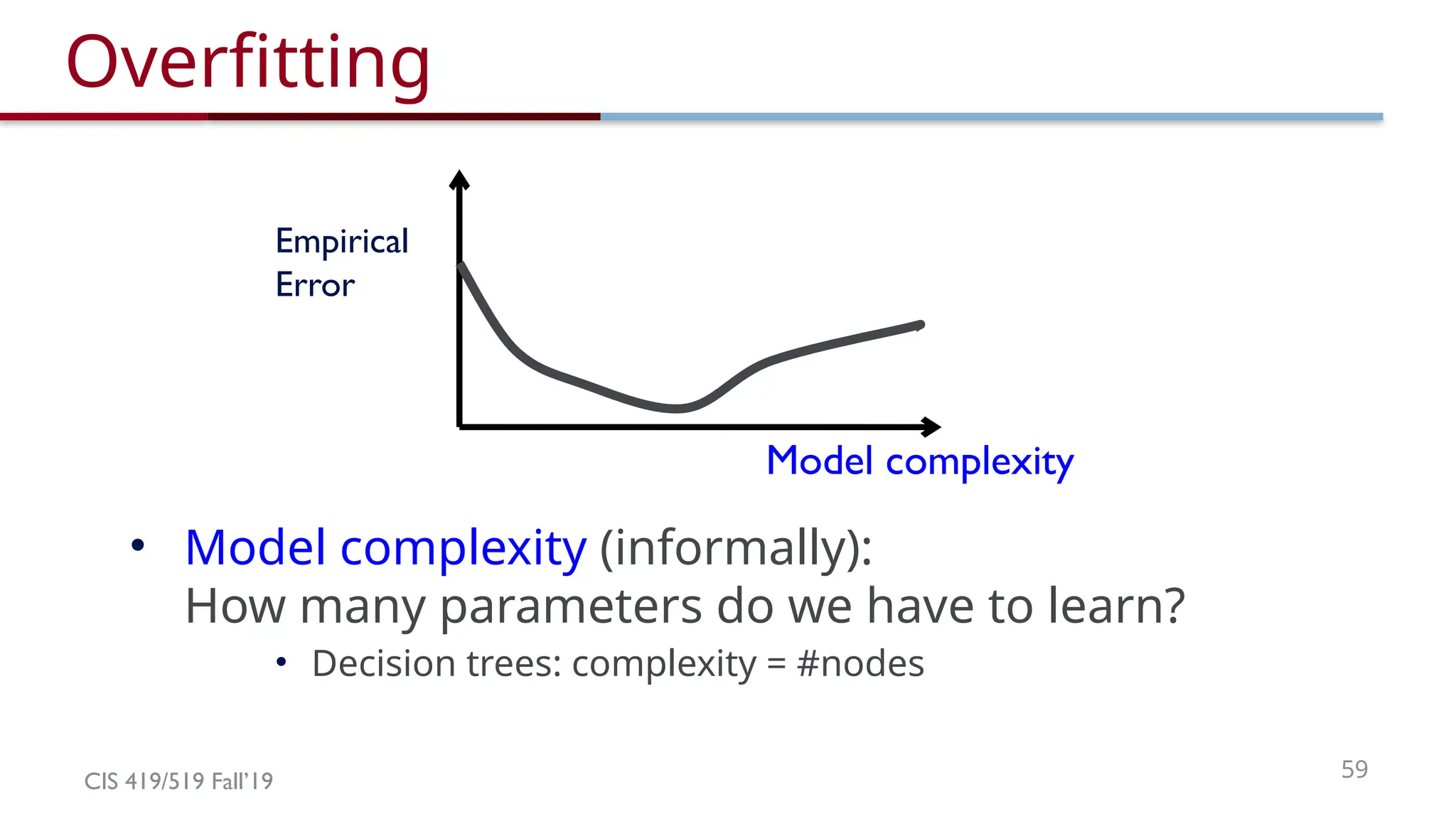
• Model complexity (informally):
How many parameters do we have to learn?
• Decision trees: complexity = #nodes

57. CIS 419/519 Fall’19 60
Model complexity
Expected
Error
Overfitting
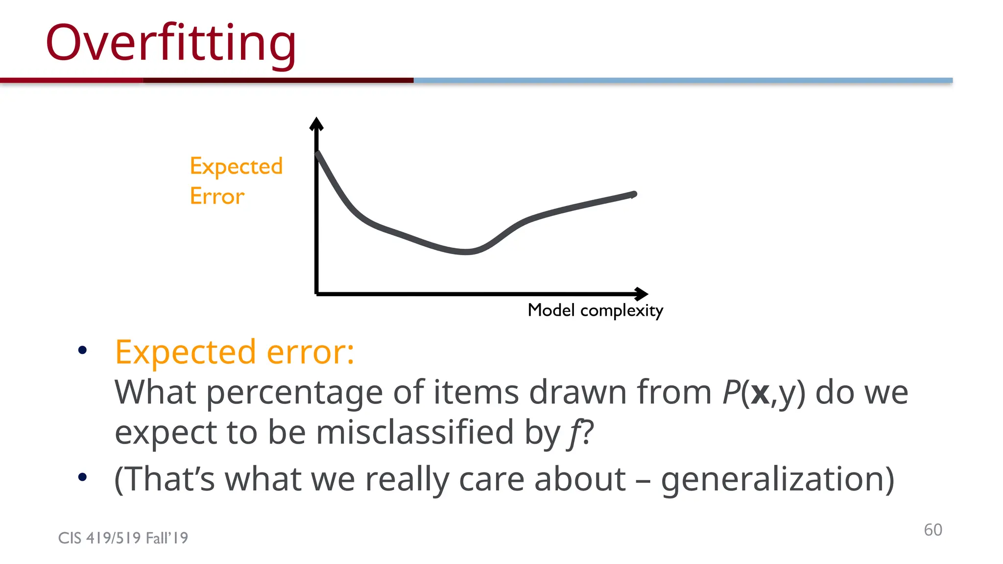
• Expected error:
What percentage of items drawn from P(x,y) do we
expect to be misclassified by f?
• (That’s what we really care about – generalization)

58. CIS 419/519 Fall’19 61
Model complexity
Variance of a learner (informally)
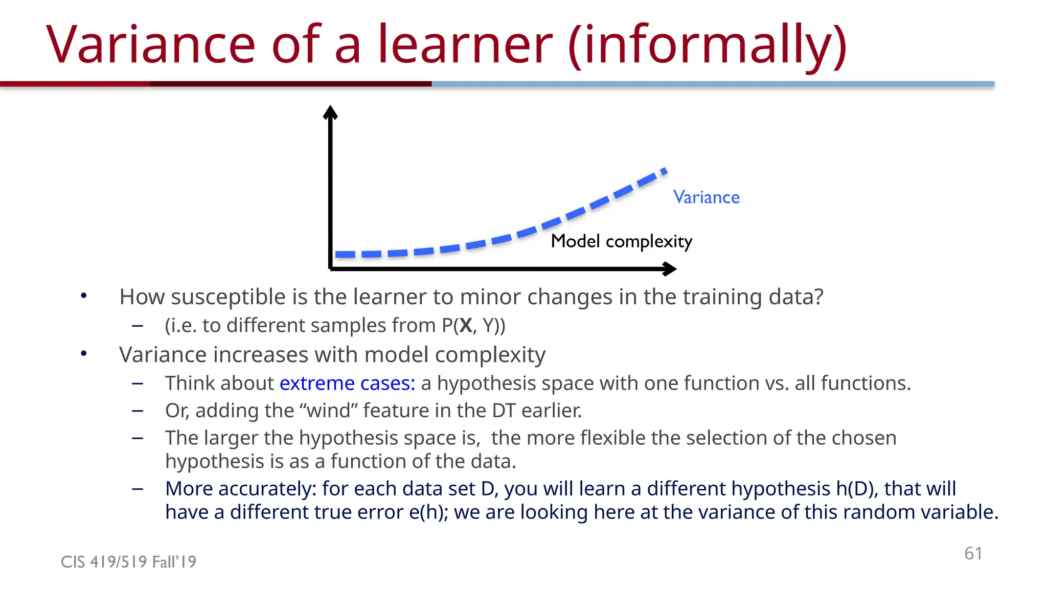
• How susceptible is the learner to minor changes in the training data?
– (i.e. to different samples from P(X, Y))
• Variance increases with model complexity
– Think about extreme cases: a hypothesis space with one function vs. all functions.
– Or, adding the “wind” feature in the DT earlier.
– The larger the hypothesis space is, the more flexible the selection of the chosen
hypothesis is as a function of the data.
– More accurately: for each data set D, you will learn a different hypothesis h(D), that will
have a different true error e(h); we are looking here at the variance of this random variable.
Variance

59. CIS 419/519 Fall’19 62
Model complexity
Bias of a learner (informally)
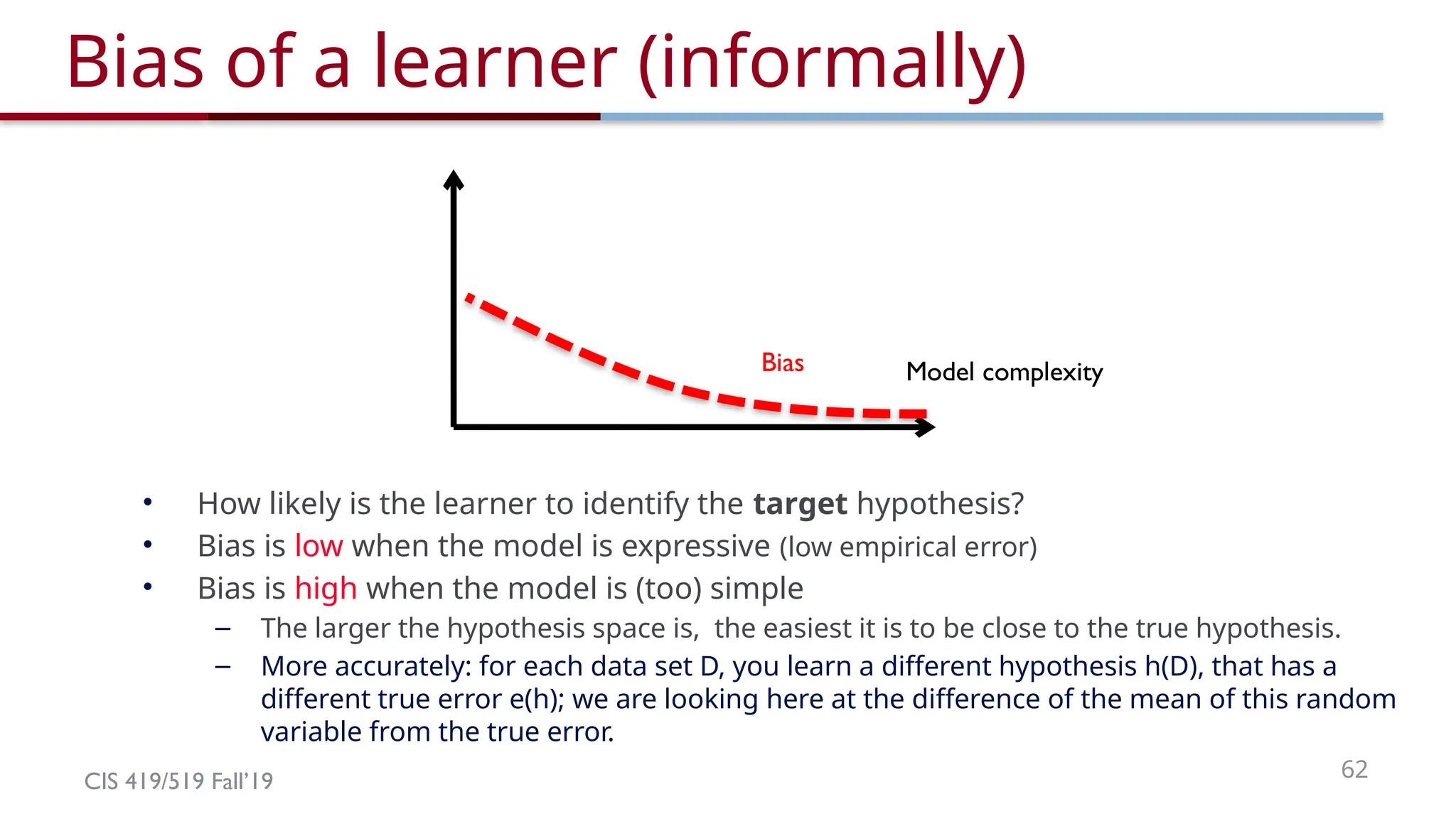
• How likely is the learner to identify the target hypothesis?
• Bias is low when the model is expressive (low empirical error)
• Bias is high when the model is (too) simple
– The larger the hypothesis space is, the easiest it is to be close to the true hypothesis.
– More accurately: for each data set D, you learn a different hypothesis h(D), that has a
different true error e(h); we are looking here at the difference of the mean of this random
variable from the true error.
Bias

60. CIS 419/519 Fall’19 63
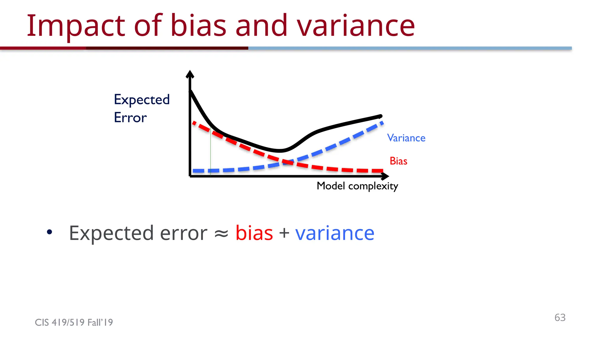
Model complexity
Expected
Error
Impact of bias and variance
• Expected error ≈ bias + variance
Variance
Bias

61. CIS 419/519 Fall’19 64
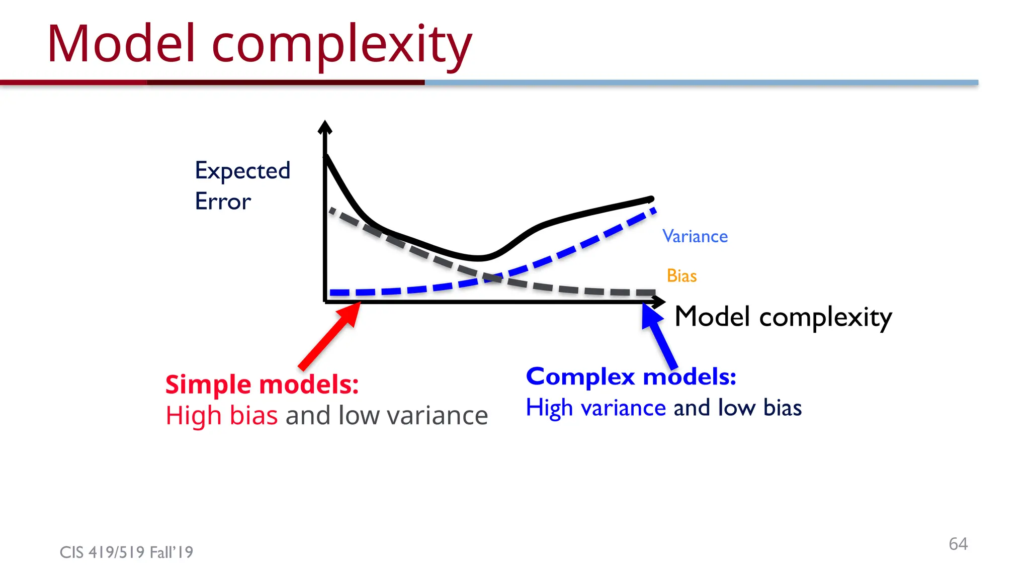
Model complexity
Expected
Error
Model complexity
Simple models:
High bias and low variance
Variance
Bias
Complex models:
High variance and low bias

62. CIS 419/519 Fall’19 65
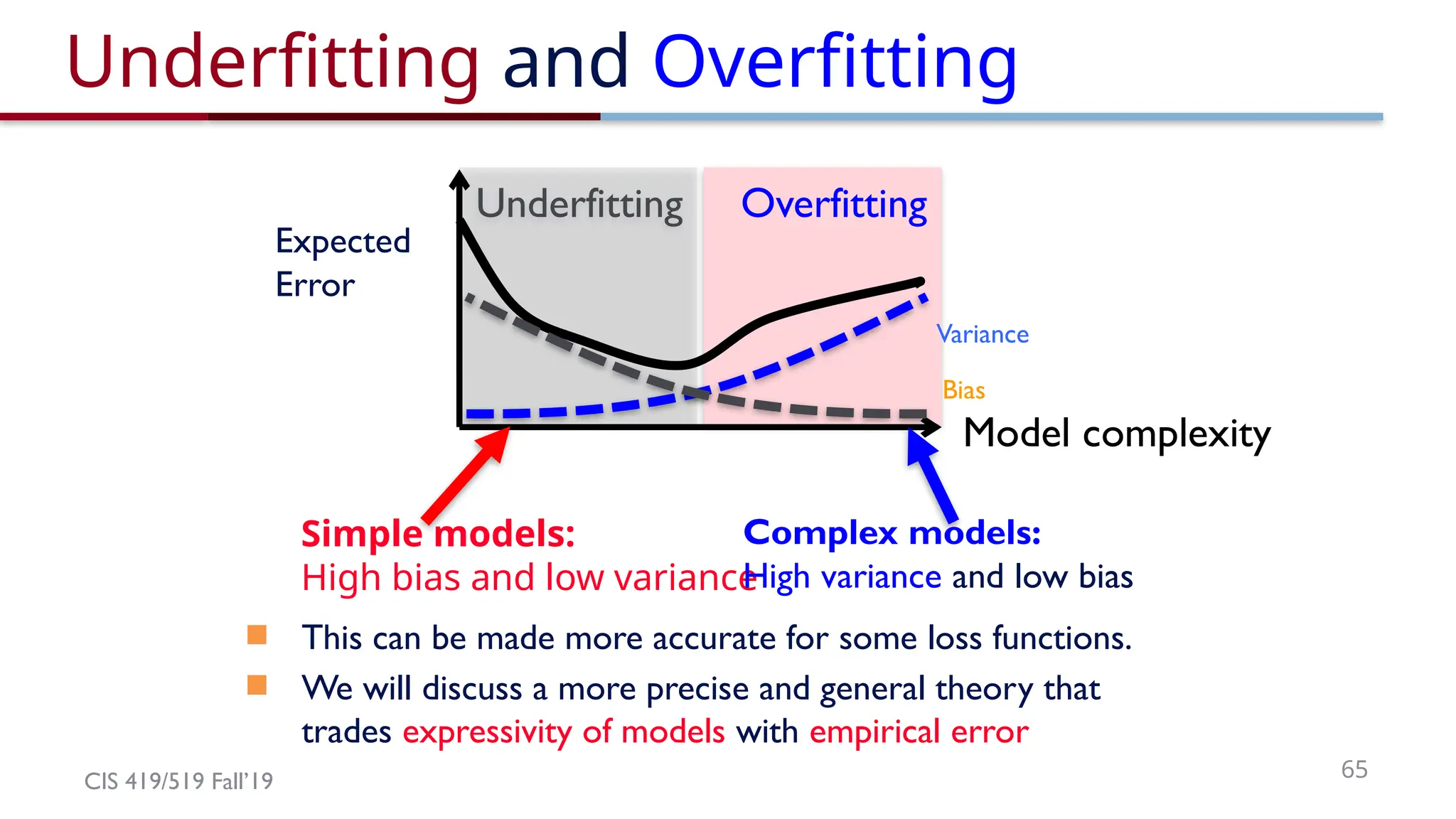
Underfitting Overfitting
Model complexity
Expected
Error
Underfitting and Overfitting
Simple models:
High bias and low variance
Variance
Bias
Complex models:
High variance and low bias
This can be made more accurate for some loss functions.
We will discuss a more precise and general theory that
trades expressivity of models with empirical error

63. CIS 419/519 Fall’19 66
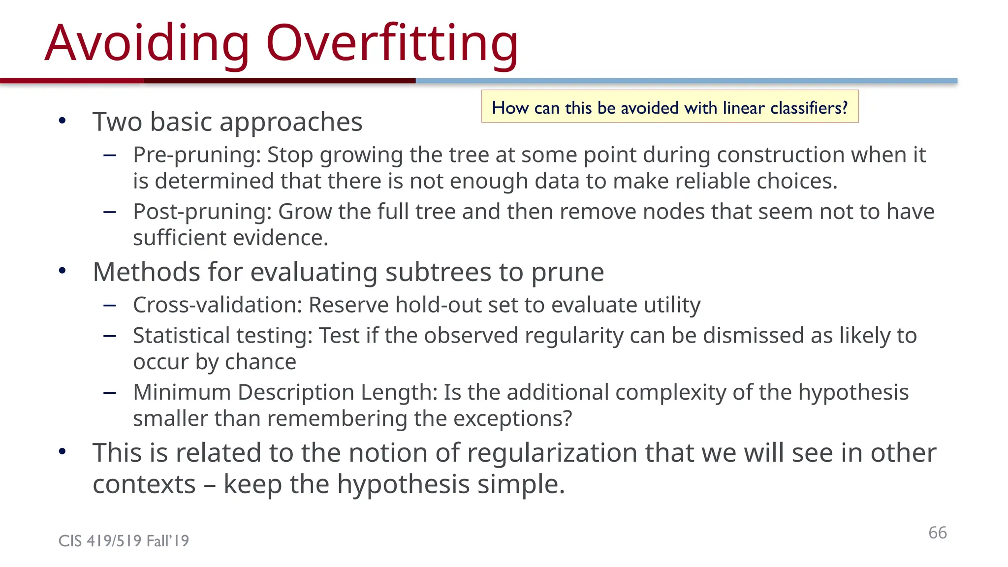
Avoiding Overfitting
• Two basic approaches
– Pre-pruning: Stop growing the tree at some point during construction when it
is determined that there is not enough data to make reliable choices.
– Post-pruning: Grow the full tree and then remove nodes that seem not to have
sufficient evidence.
• Methods for evaluating subtrees to prune
– Cross-validation: Reserve hold-out set to evaluate utility
– Statistical testing: Test if the observed regularity can be dismissed as likely to
occur by chance
– Minimum Description Length: Is the additional complexity of the hypothesis
smaller than remembering the exceptions?
• This is related to the notion of regularization that we will see in other
contexts – keep the hypothesis simple.
How can this be avoided with linear classifiers?

64. CIS 419/519 Fall’19 67
Trees and Rules
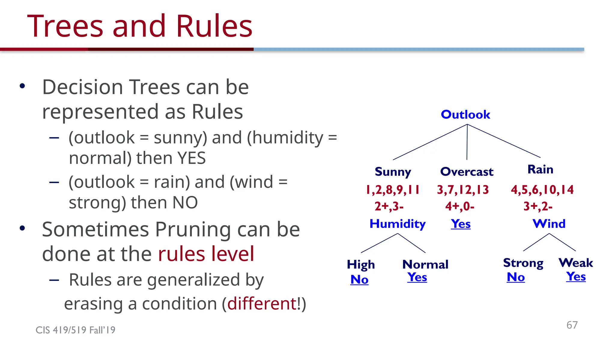
• Decision Trees can be
represented as Rules
– (outlook = sunny) and (humidity =
normal) then YES
– (outlook = rain) and (wind =
strong) then NO
• Sometimes Pruning can be
done at the rules level
– Rules are generalized by
erasing a condition (different!)
Outlook
Overcast Rain
3,7,12,13 4,5,6,10,14
3+,2-
Sunny
1,2,8,9,11
4+,0-
2+,3-
Yes
Humidity Wind
Normal
High
No
Weak
Strong
No Yes
Yes

65. CIS 419/519 Fall’19
DT Extensions:
continuous attributes and
missing values

66. CIS 419/519 Fall’19 69
Continuous Attributes
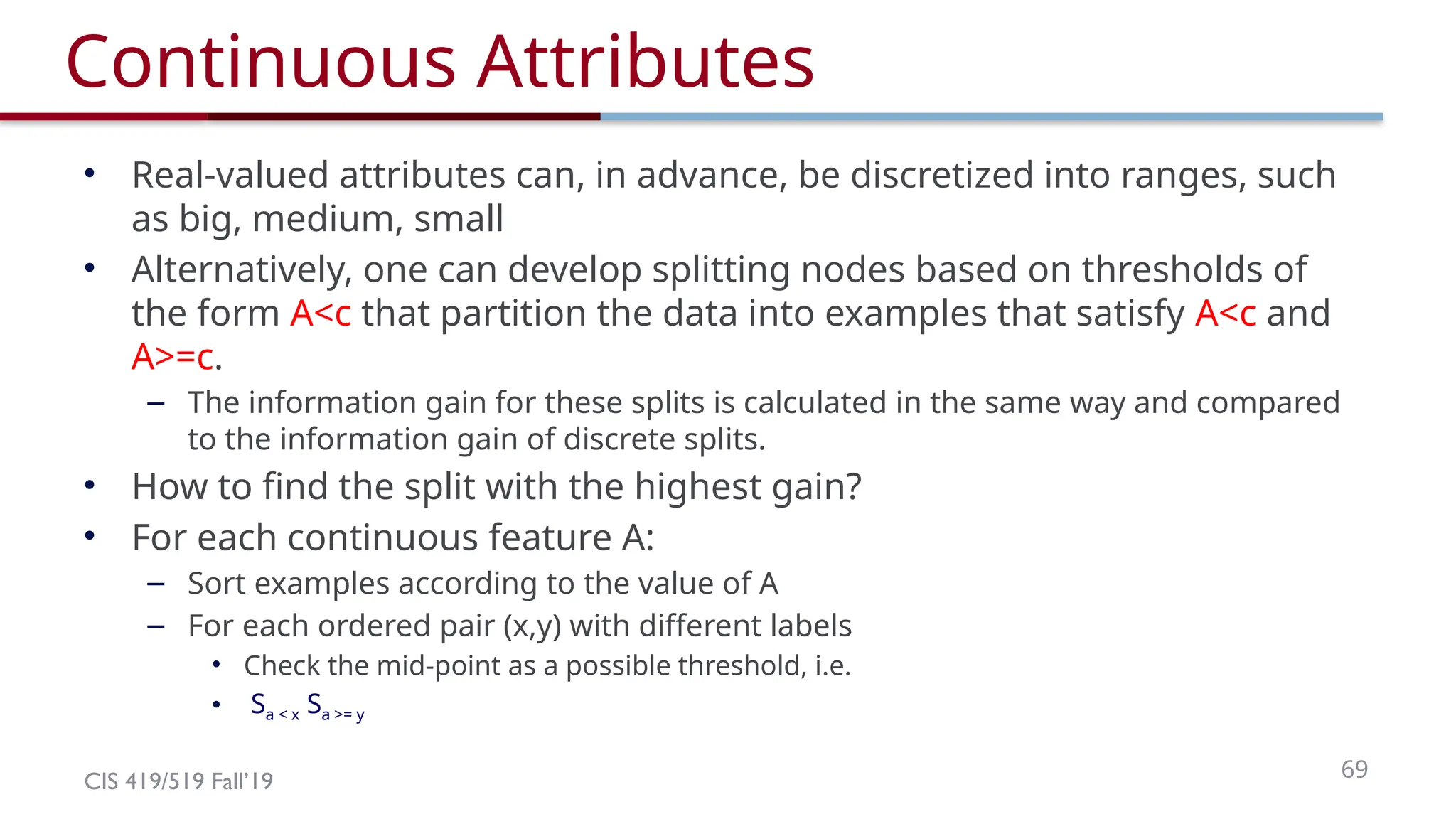
• Real-valued attributes can, in advance, be discretized into ranges, such
as big, medium, small
• Alternatively, one can develop splitting nodes based on thresholds of
the form A<c that partition the data into examples that satisfy A<c and
A>=c.
– The information gain for these splits is calculated in the same way and compared
to the information gain of discrete splits.
• How to find the split with the highest gain?
• For each continuous feature A:
– Sort examples according to the value of A
– For each ordered pair (x,y) with different labels
• Check the mid-point as a possible threshold, i.e.
• Sa < x Sa >= y

67. CIS 419/519 Fall’19 70
Continuous Attributes
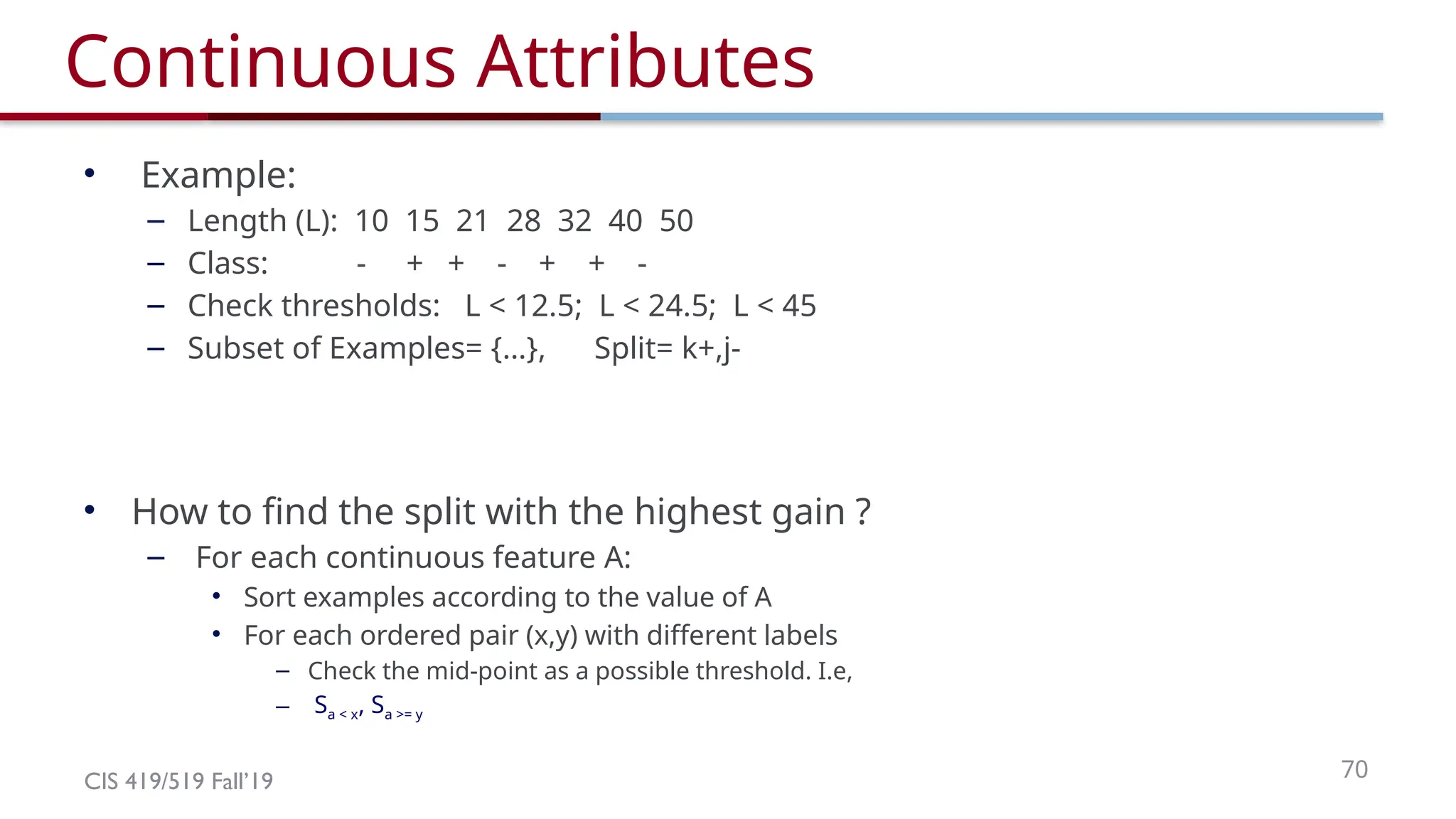
• Example:
– Length (L): 10 15 21 28 32 40 50
– Class: - + + - + + -
– Check thresholds: L < 12.5; L < 24.5; L < 45
– Subset of Examples= {…}, Split= k+,j-
• How to find the split with the highest gain ?
– For each continuous feature A:
• Sort examples according to the value of A
• For each ordered pair (x,y) with different labels
– Check the mid-point as a possible threshold. I.e,
– Sa < x, Sa >= y

68. CIS 419/519 Fall’19 71
Missing Values
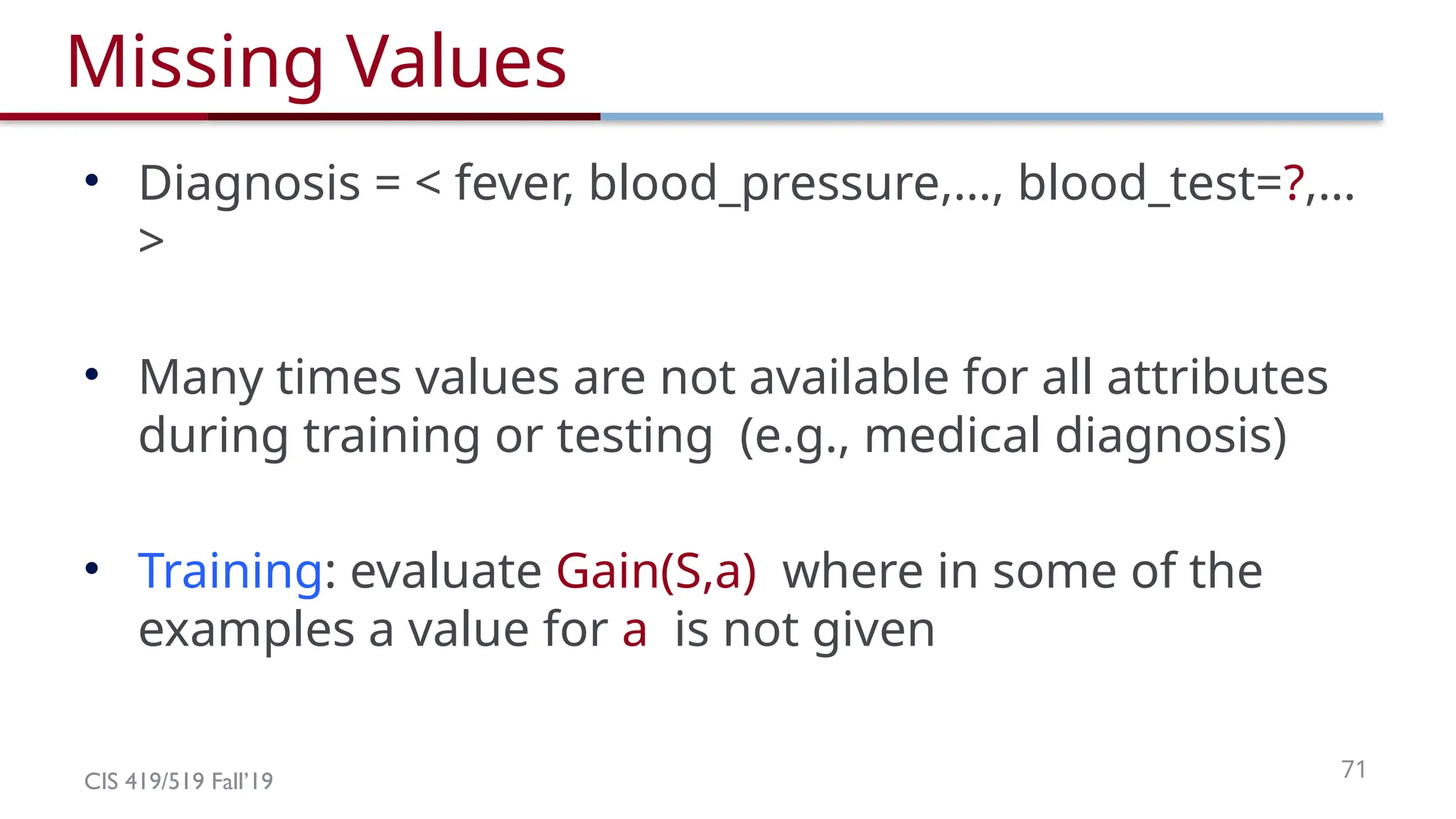
• Diagnosis = < fever, blood_pressure,…, blood_test=?,…
>
• Many times values are not available for all attributes
during training or testing (e.g., medical diagnosis)
• Training: evaluate Gain(S,a) where in some of the
examples a value for a is not given

69. CIS 419/519 Fall’19
Missing Values
Outlook
Overcast Rain
3,7,12,134,5,6,10,14
3+,2-
Sunny
1,2,8,9,11
4+,0-
2+,3-
Yes
? ?

Humidity)
,
Gain(Ssunny

Temp)
,
Gain(Ssunny .97- 0-(2/5) 1 = .57
Day Outlook Temperature Humidity Wind PlayTennis
1 Sunny Hot High Weak No
2 Sunny Hot High Strong No
8 Sunny Mild ??? Weak No
9 Sunny Cool Normal Weak Yes
11 Sunny Mild Normal Strong Yes
 Fill in: assign the most likely value of Xi to s:
argmax k P( Xi = k ):
Normal
 97-(3/5) Ent[+0,-3] -(2/5) Ent[+2,-0] = .97
 Assign fractional counts P(Xi =k)
for each value of Xi to s
 .97-(2.5/5) Ent[+0,-2.5] - (2.5/5) Ent[+2,-.5] < .97
Other suggestions?
𝐺𝑎𝑖𝑛(𝑆,𝑎)=𝐸𝑛𝑡𝑟𝑜𝑝𝑦(𝑆)−∑¿𝑆𝑣∨ ¿
¿𝑆∨¿𝐸𝑛𝑡𝑟𝑜𝑝𝑦(𝑆𝑣)
¿¿

70. CIS 419/519 Fall’19 73
Missing Values
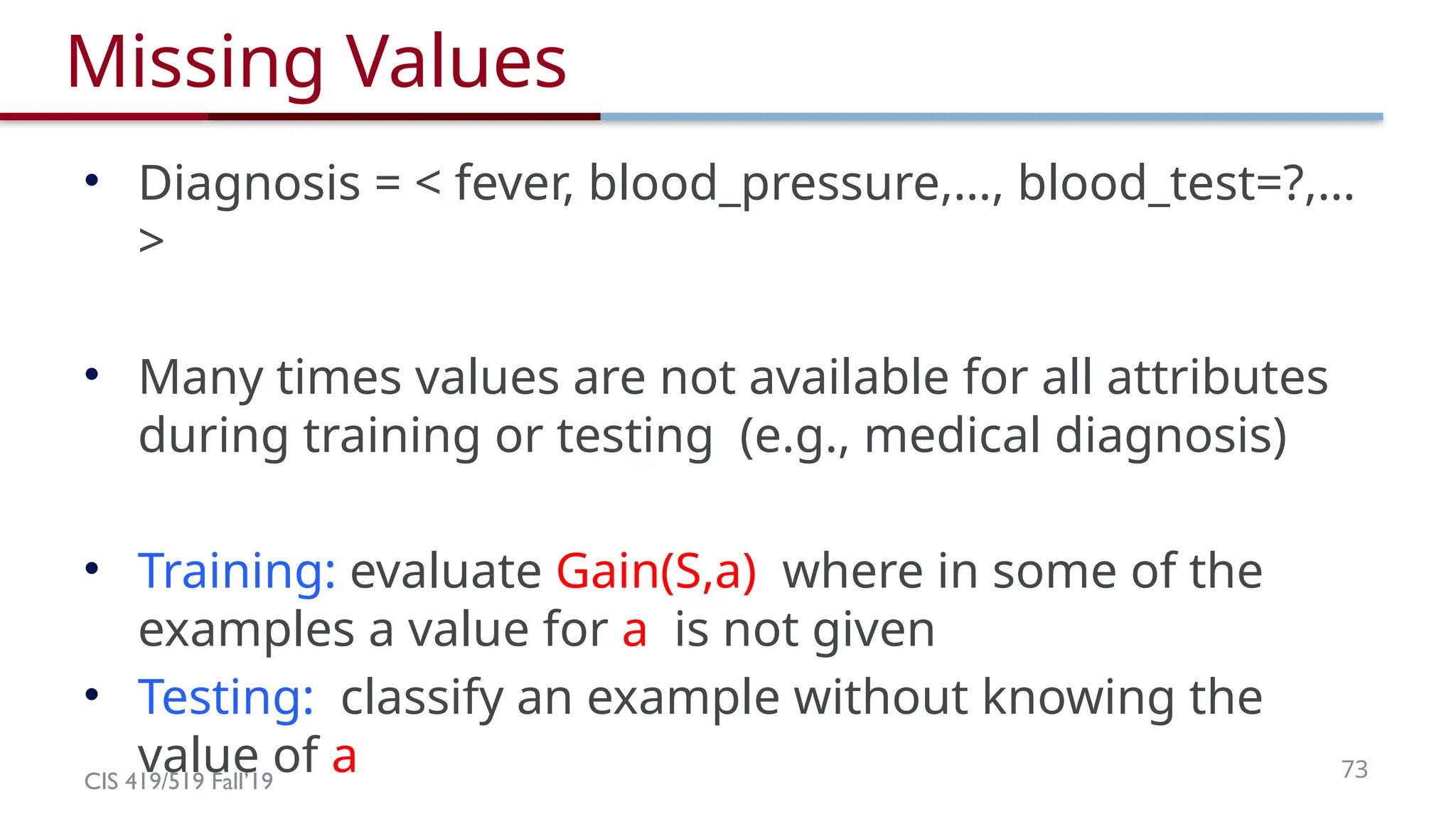
• Diagnosis = < fever, blood_pressure,…, blood_test=?,…
>
• Many times values are not available for all attributes
during training or testing (e.g., medical diagnosis)
• Training: evaluate Gain(S,a) where in some of the
examples a value for a is not given
• Testing: classify an example without knowing the
value of a

71. CIS 419/519 Fall’19 74
MissingValues
Outlook
Overcast Rain
3,7,12,13 4,5,6,10,14
3+,2-
Sunny
1,2,8,9,11
4+,0-
2+,3-
Yes
Humidity Wind
Normal
High
No
Weak
Strong
No Yes
Yes
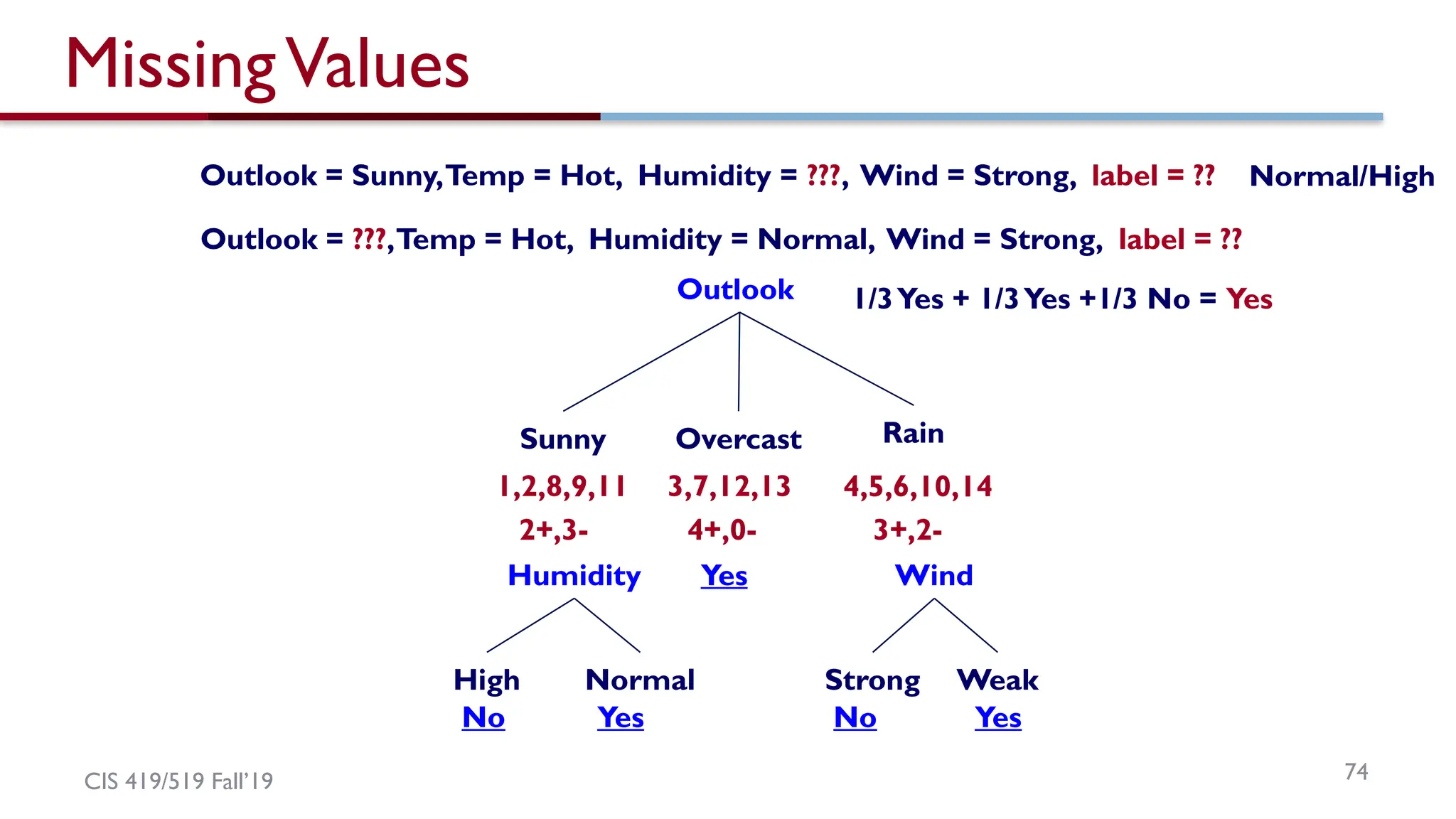
Outlook = ???,Temp = Hot, Humidity = Normal, Wind = Strong, label = ??
1/3Yes + 1/3Yes +1/3 No = Yes
Outlook = Sunny,Temp = Hot, Humidity = ???, Wind = Strong, label = ?? Normal/High

72. CIS 419/519 Fall’19 75
Other Issues
• Attributes with different costs
– Change information gain so that low cost attribute are preferred
• Dealing with features with different # of values
• Alternative measures for selecting attributes
– When different attributes have different number of values
information gain tends to prefer those with many values
• Oblique Decision Trees
– Decisions are not axis-parallel
• Incremental Decision Trees induction
– Update an existing decision tree to account for new examples
incrementally (Maintain consistency?)

73. CIS 419/519 Fall’19 76
Summary: Decision Trees
• Presented the hypothesis class of Decision Trees
– Very expressive, flexible, class of functions
• Presented a learning algorithm for Decision Tress
– Recursive algorithm.
– Key step is based on the notion of Entropy
• Discussed the notion of overfitting and ways to address it within DTs
– In your problem set – look at the performance on the training vs. test
• Briefly discussed some extensions
– Real valued attributes
– Missing attributes
• Evaluation in machine learning
– Cross validation
– Statistical significance

74. CIS 419/519 Fall’19 77
Decision Trees as Features
• Rather than using decision trees to represent the target function it is becoming
common to use small decision trees as features
• When learning over a large number of features, learning decision trees is difficult and
the resulting tree may be very large
 (over fitting)
• Instead, learn small decision trees, with limited depth.
• Treat them as “experts”; they are correct, but only on a small region in the domain.
(what DTs to learn? same every time?)
• Then, learn another function, typically a linear function, over these as features.
• Boosting (but also other linear learners) are used on top of the small decision trees.
(Either Boolean, or real valued features)
• In HW1 you learn a linear classifier over DTs.
– Not learning the DTs sequentially; all are learned at once.
• How can you learn multiple DTs?
– Combining them using an SGD algorithm.

75. CIS 419/519 Fall’19 78
Experimental Machine Learning
• Machine Learning is an Experimental Field and we will spend some
time (in Problem sets) learning how to run experiments and evaluate
results
– First hint: be organized; write scripts
• Basics:
– Split your data into three sets:
• Training data (often 70-90%)
• Test data (often 10-20%)
• Development data (10-20%)
• You need to report performance on test data, but you are not allowed
to look at it.
– You are allowed to look at the development data (and use it to tune
parameters)

76. CIS 419/519 Fall’19
Metrics
Methodologies
Statistical Significance

77. CIS 419/519 Fall’19 80
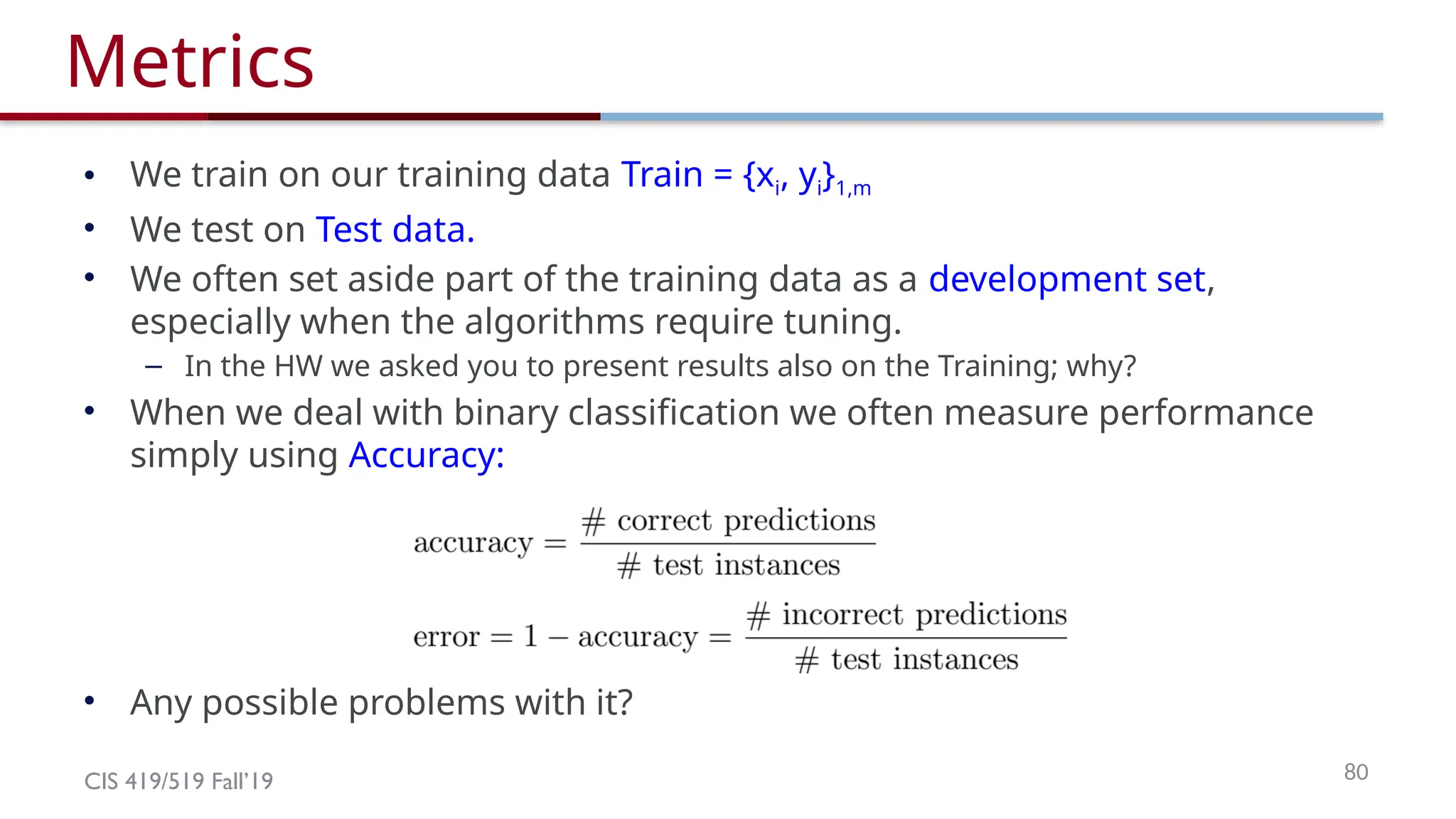
Metrics
• We train on our training data Train = {xi, yi}1,m
• We test on Test data.
• We often set aside part of the training data as a development set,
especially when the algorithms require tuning.
– In the HW we asked you to present results also on the Training; why?
• When we deal with binary classification we often measure performance
simply using Accuracy:
• Any possible problems with it?

78. CIS 419/519 Fall’19 81
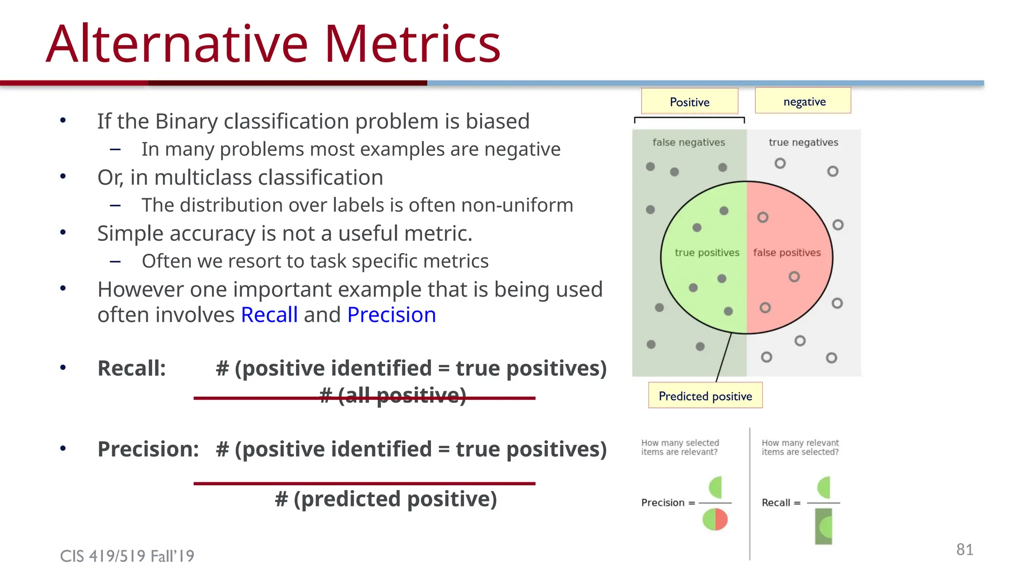
Alternative Metrics
• If the Binary classification problem is biased
– In many problems most examples are negative
• Or, in multiclass classification
– The distribution over labels is often non-uniform
• Simple accuracy is not a useful metric.
– Often we resort to task specific metrics
• However one important example that is being used
often involves Recall and Precision
• Recall: # (positive identified = true positives)
# (all positive)
• Precision: # (positive identified = true positives)
# (predicted positive)
Predicted positive
Positive negative

79. CIS 419/519 Fall’19 82
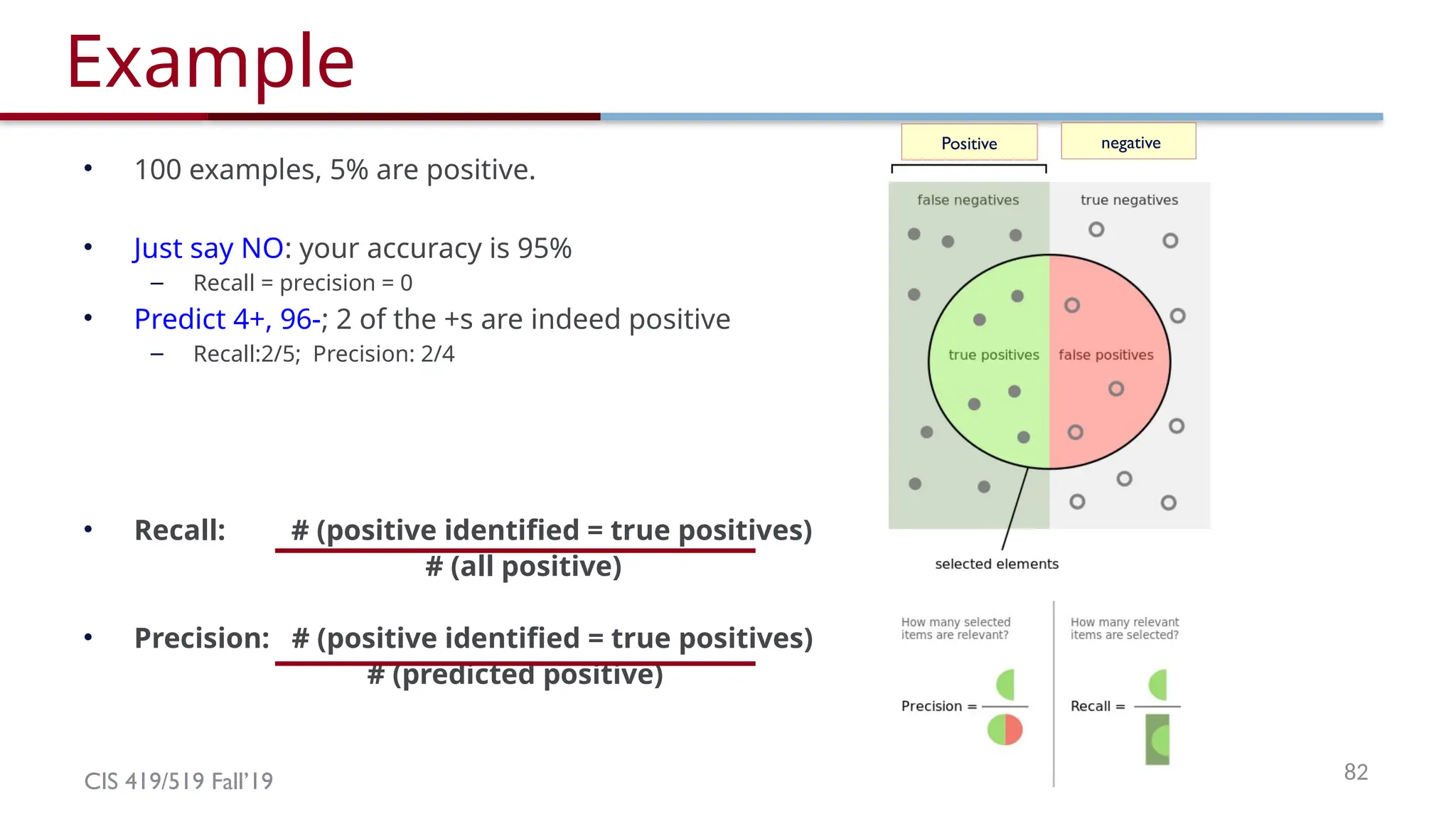
Example
• 100 examples, 5% are positive.
• Just say NO: your accuracy is 95%
– Recall = precision = 0
• Predict 4+, 96-; 2 of the +s are indeed positive
– Recall:2/5; Precision: 2/4
• Recall: # (positive identified = true positives)
# (all positive)
• Precision: # (positive identified = true positives)
# (predicted positive)
Positive negative

80. CIS 419/519 Fall’19
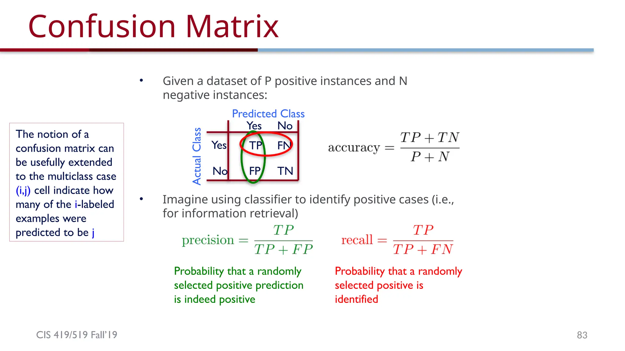
Confusion Matrix
83
• Given a dataset of P positive instances and N
negative instances:
• Imagine using classifier to identify positive cases (i.e.,
for information retrieval)
Yes
No
Yes No
Actual
Class
Predicted Class
TP FN
FP TN
Probability that a randomly
selected positive prediction
is indeed positive
Probability that a randomly
selected positive is
identified
The notion of a
confusion matrix can
be usefully extended
to the multiclass case
(i,j) cell indicate how
many of the i-labeled
examples were
predicted to be j

81. CIS 419/519 Fall’19 84
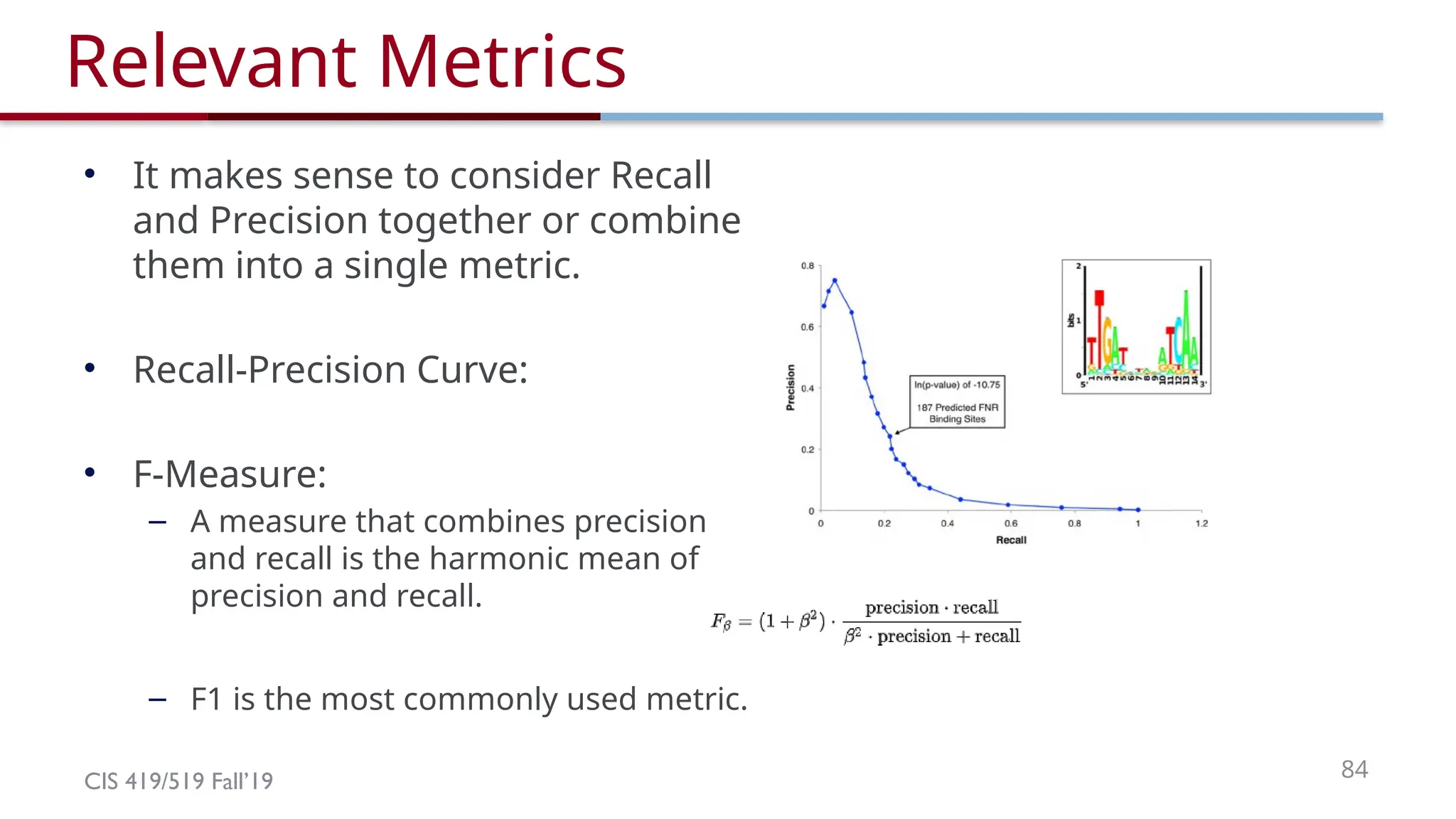
Relevant Metrics
• It makes sense to consider Recall
and Precision together or combine
them into a single metric.
• Recall-Precision Curve:
• F-Measure:
– A measure that combines precision
and recall is the harmonic mean of
precision and recall.
– F1 is the most commonly used metric.

82. CIS 419/519 Fall’19 85
Comparing Classifiers
Say we have two classifiers, C1 and C2, and want to
choose the best one to use for future predictions
Can we use training accuracy to choose between them?
• No!
• What about accuracy on test data?

83. CIS 419/519 Fall’19 86
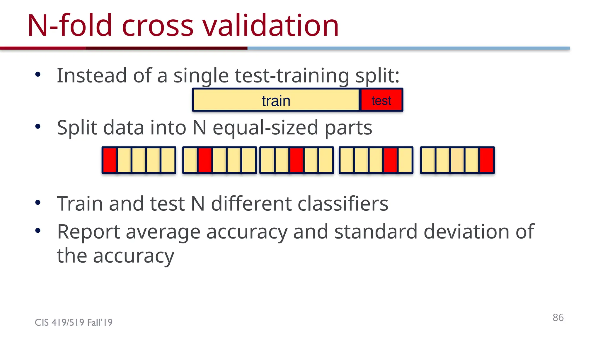
N-fold cross validation
• Instead of a single test-training split:
• Split data into N equal-sized parts
• Train and test N different classifiers
• Report average accuracy and standard deviation of
the accuracy
train test

84. CIS 419/519 Fall’19 87
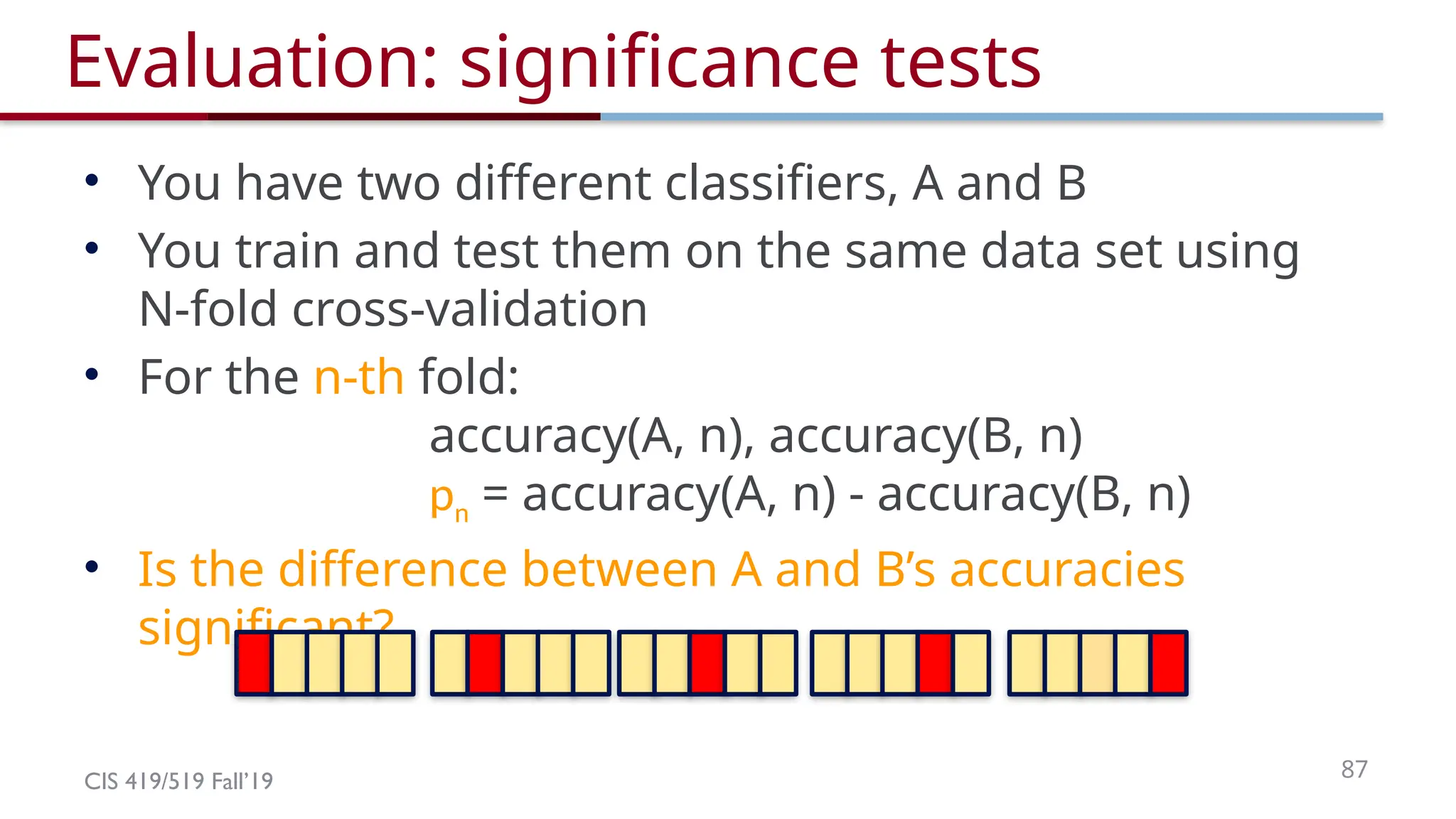
Evaluation: significance tests
• You have two different classifiers, A and B
• You train and test them on the same data set using
N-fold cross-validation
• For the n-th fold:
accuracy(A, n), accuracy(B, n)
pn = accuracy(A, n) - accuracy(B, n)
• Is the difference between A and B’s accuracies
significant?

85. CIS 419/519 Fall’19 88
Hypothesis testing
• You want to show that hypothesis H is true, based on
your data
– (e.g. H = “classifier A and B are different”)
• Define a null hypothesis H0
– (H0 is the contrary of what you want to show)
• H0 defines a distribution P(m |H0) over some statistic
– e.g. a distribution over the difference in accuracy between A
and B
• Can you refute (reject) H0?

86. CIS 419/519 Fall’19 89
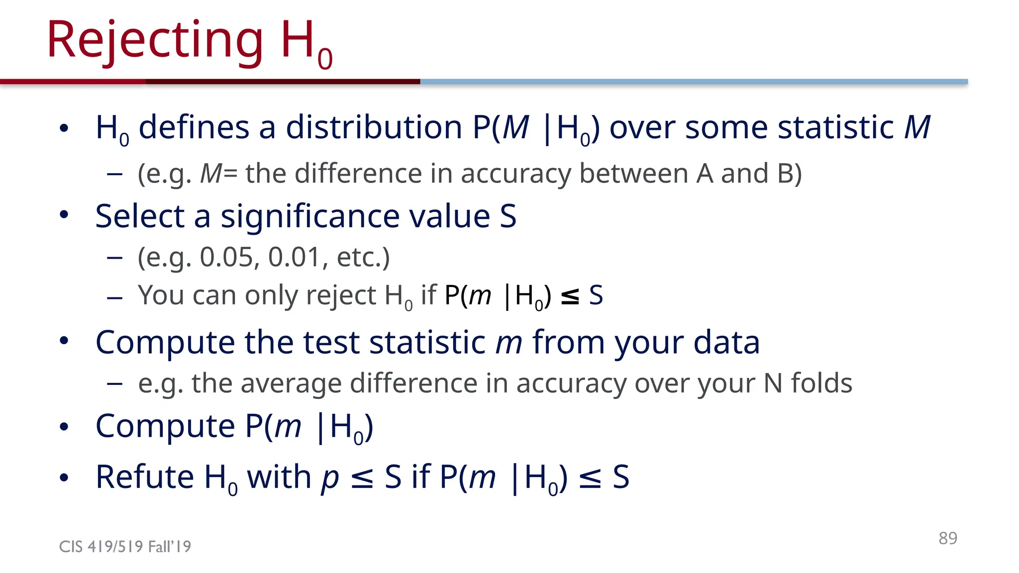
Rejecting H0
• H0 defines a distribution P(M |H0) over some statistic M
– (e.g. M= the difference in accuracy between A and B)
• Select a significance value S
– (e.g. 0.05, 0.01, etc.)
– You can only reject H0 if P(m |H0) ≤ S
• Compute the test statistic m from your data
– e.g. the average difference in accuracy over your N folds
• Compute P(m |H0)
• Refute H0 with p S if P(
≤ m |H0) S
≤

87. CIS 419/519 Fall’19 90
Paired t-test
• Null hypothesis (H0; to be refuted):
– There is no difference between A and B, i.e. the expected
accuracies of A and B are the same
• That is, the expected difference (over all possible data
sets) between their accuracies is 0:
H0: E[pD] = 0
•We don’t know the true E[pD]
•N-fold cross-validation gives us N samples of pD

88. CIS 419/519 Fall’19 91
Paired t-test
• Null hypothesis H0: E[diffD] = μ = 0
• m: our estimate of μ based on N samples of diffD
m = 1/N n diffn
•The estimated variance S2
:
S2
= 1/(N-1) 1,N (diffn – m)2
•Accept Null hypothesis at significance level a if the
following statistic lies in (-ta/2, N-1, +ta/2, N-1)

89. CIS 419/519 Fall’19 92
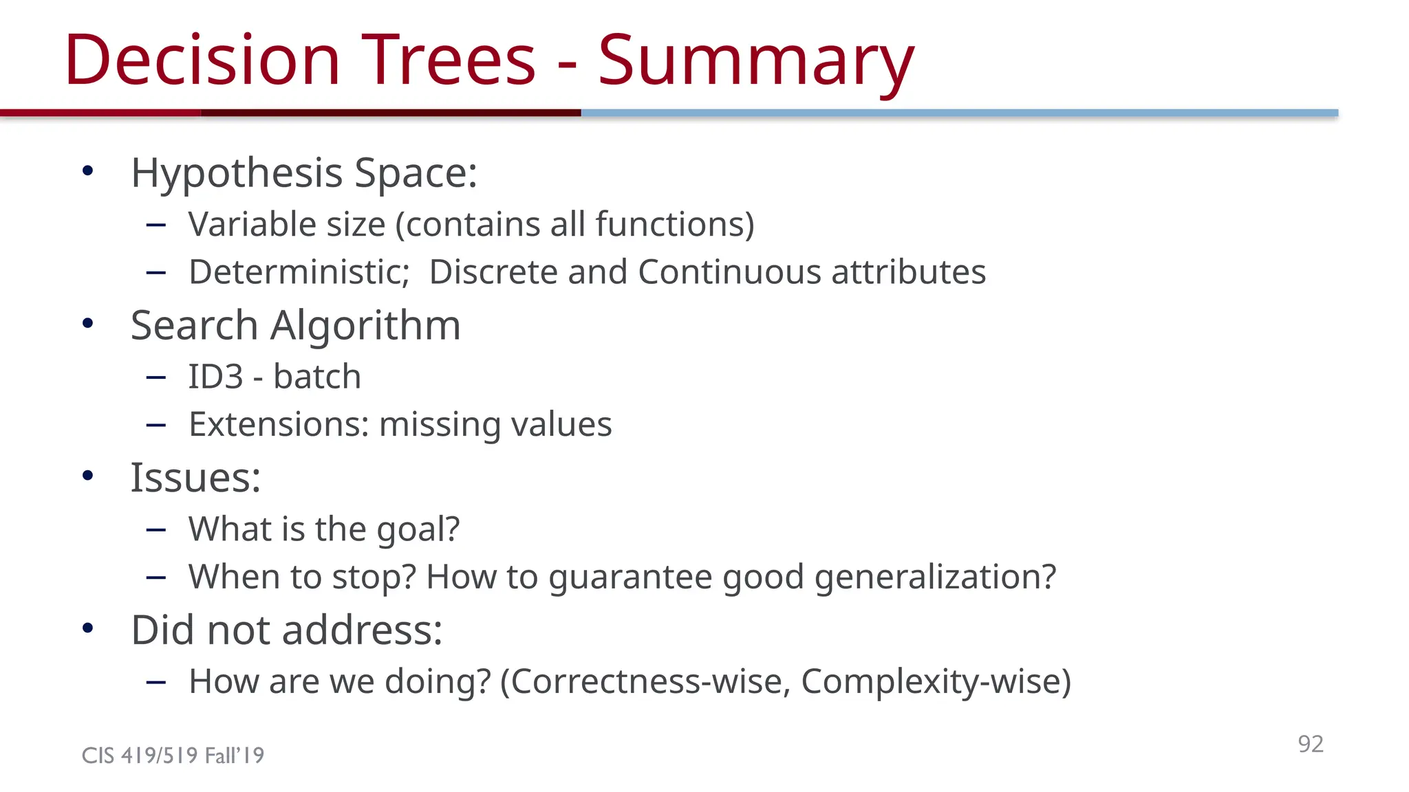
Decision Trees - Summary
• Hypothesis Space:
– Variable size (contains all functions)
– Deterministic; Discrete and Continuous attributes
• Search Algorithm
– ID3 - batch
– Extensions: missing values
• Issues:
– What is the goal?
– When to stop? How to guarantee good generalization?
• Did not address:
– How are we doing? (Correctness-wise, Complexity-wise)