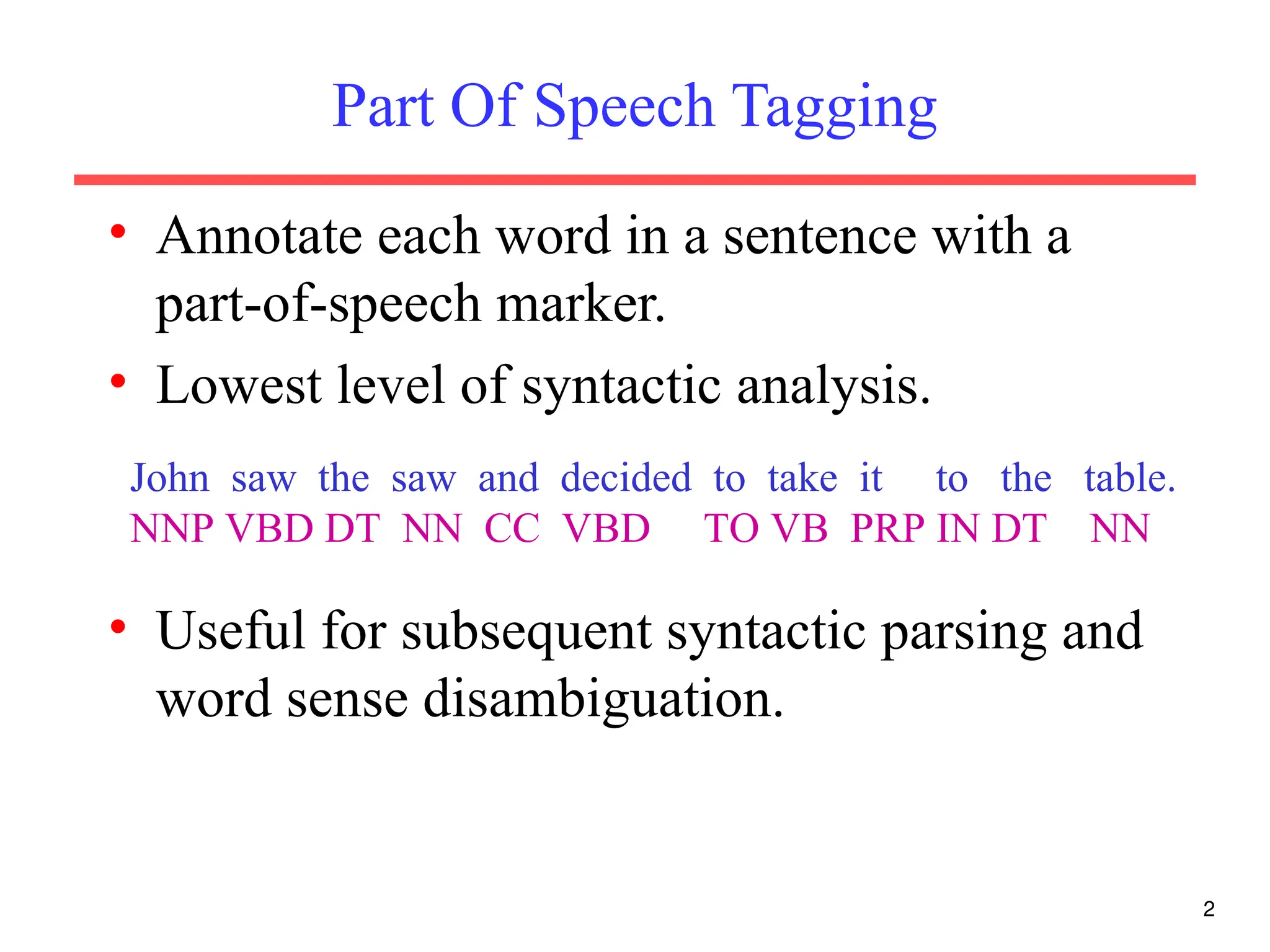
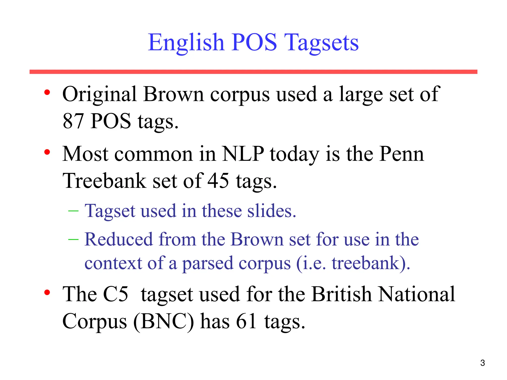
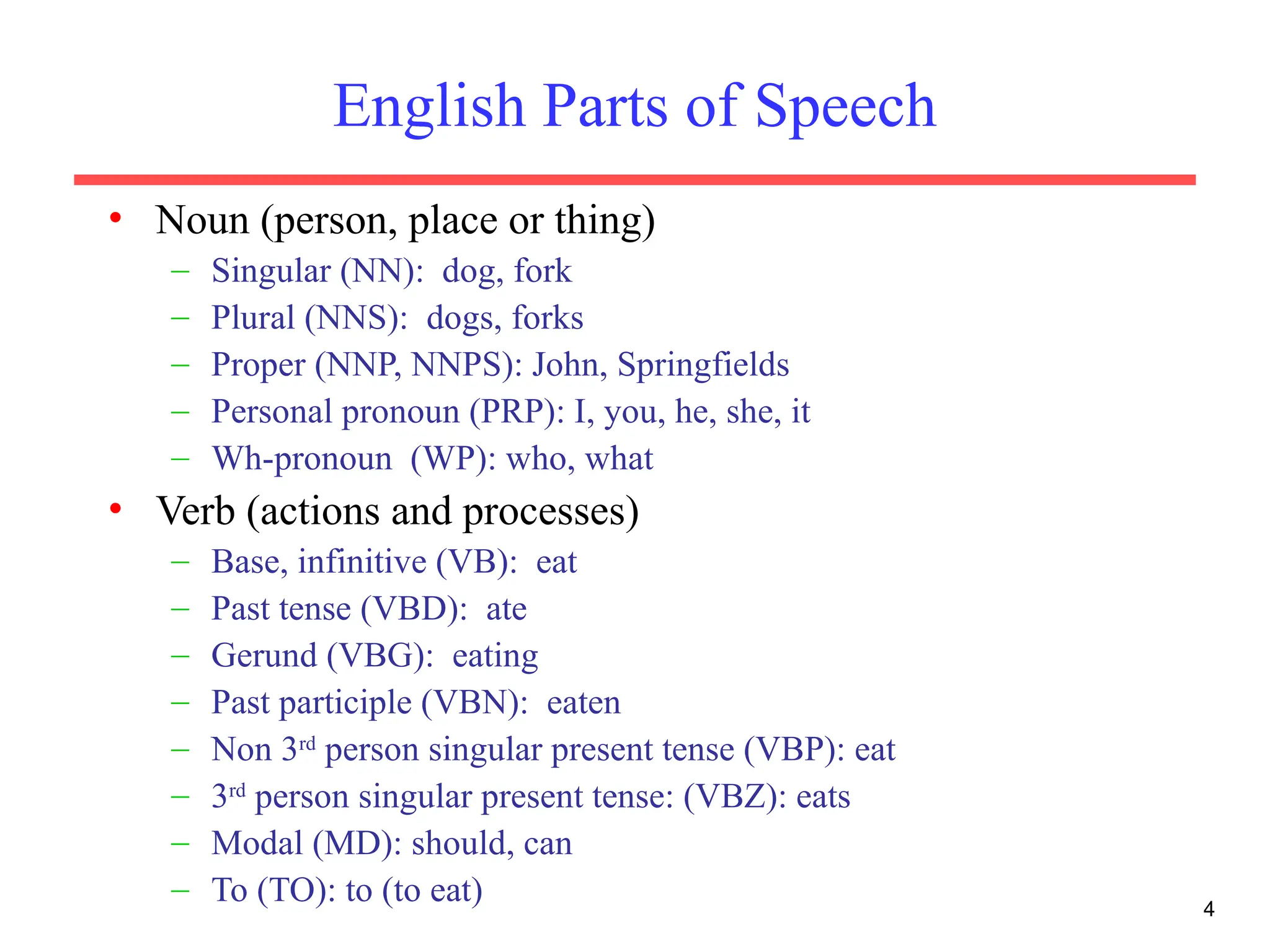
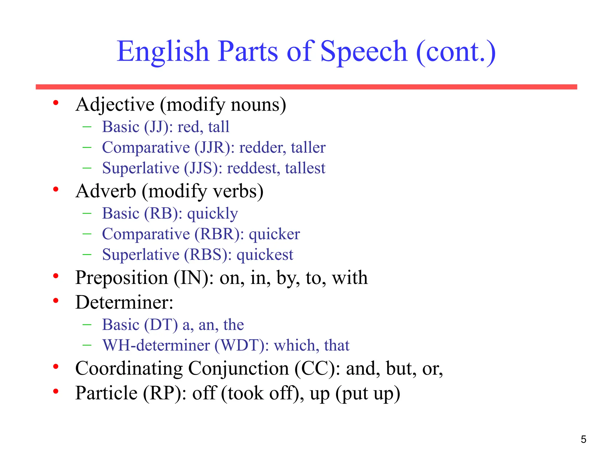
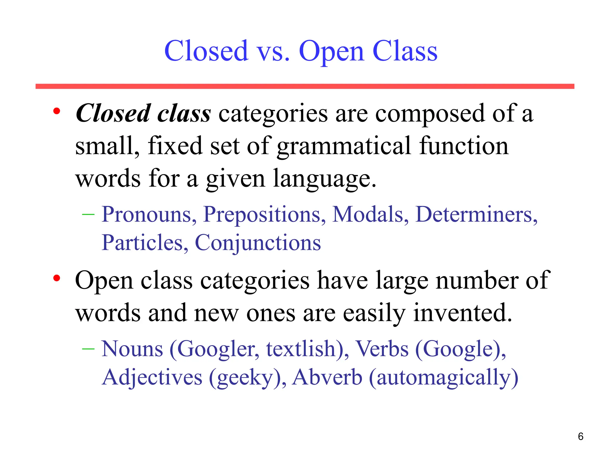
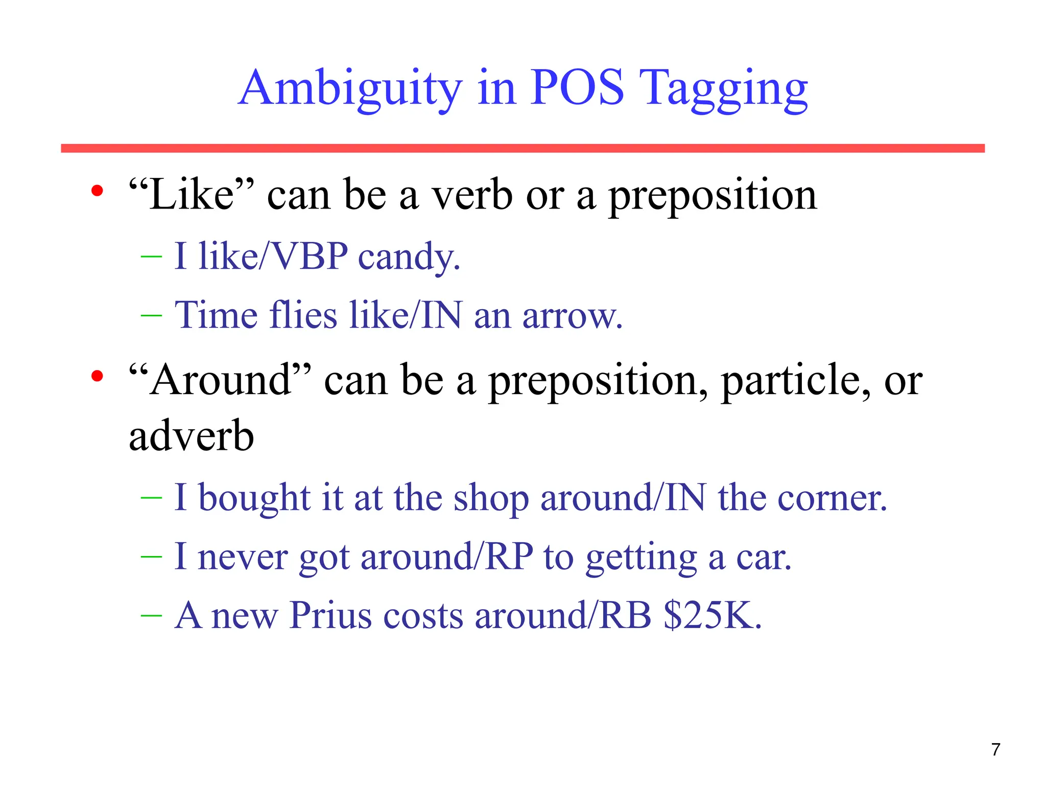
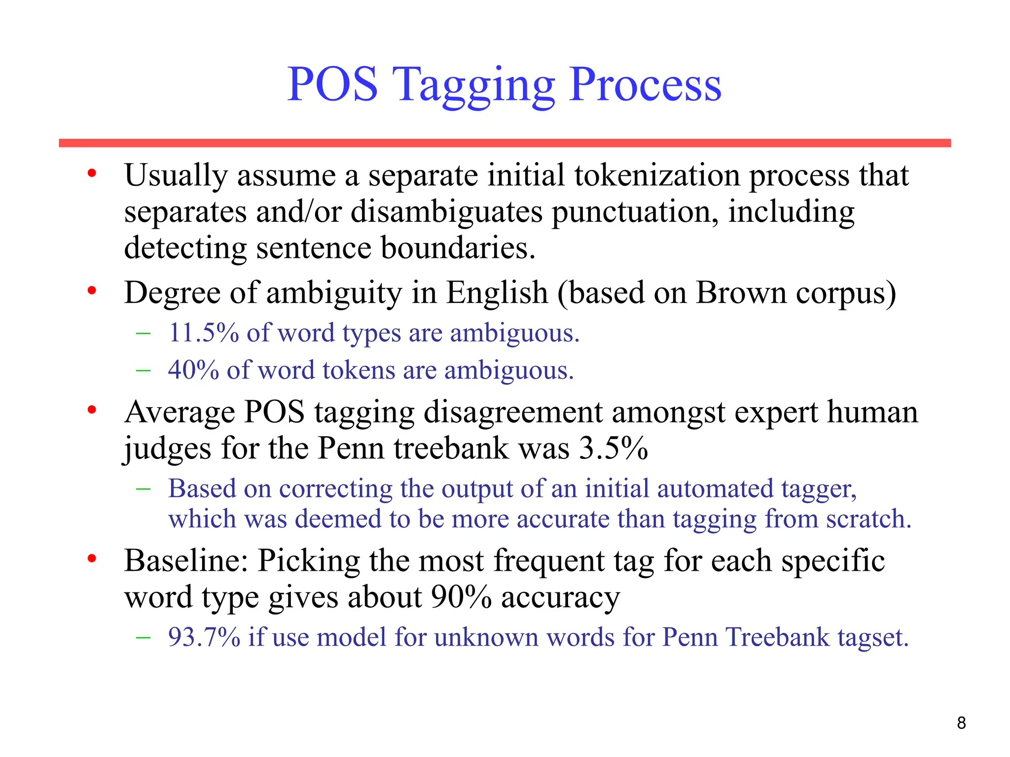
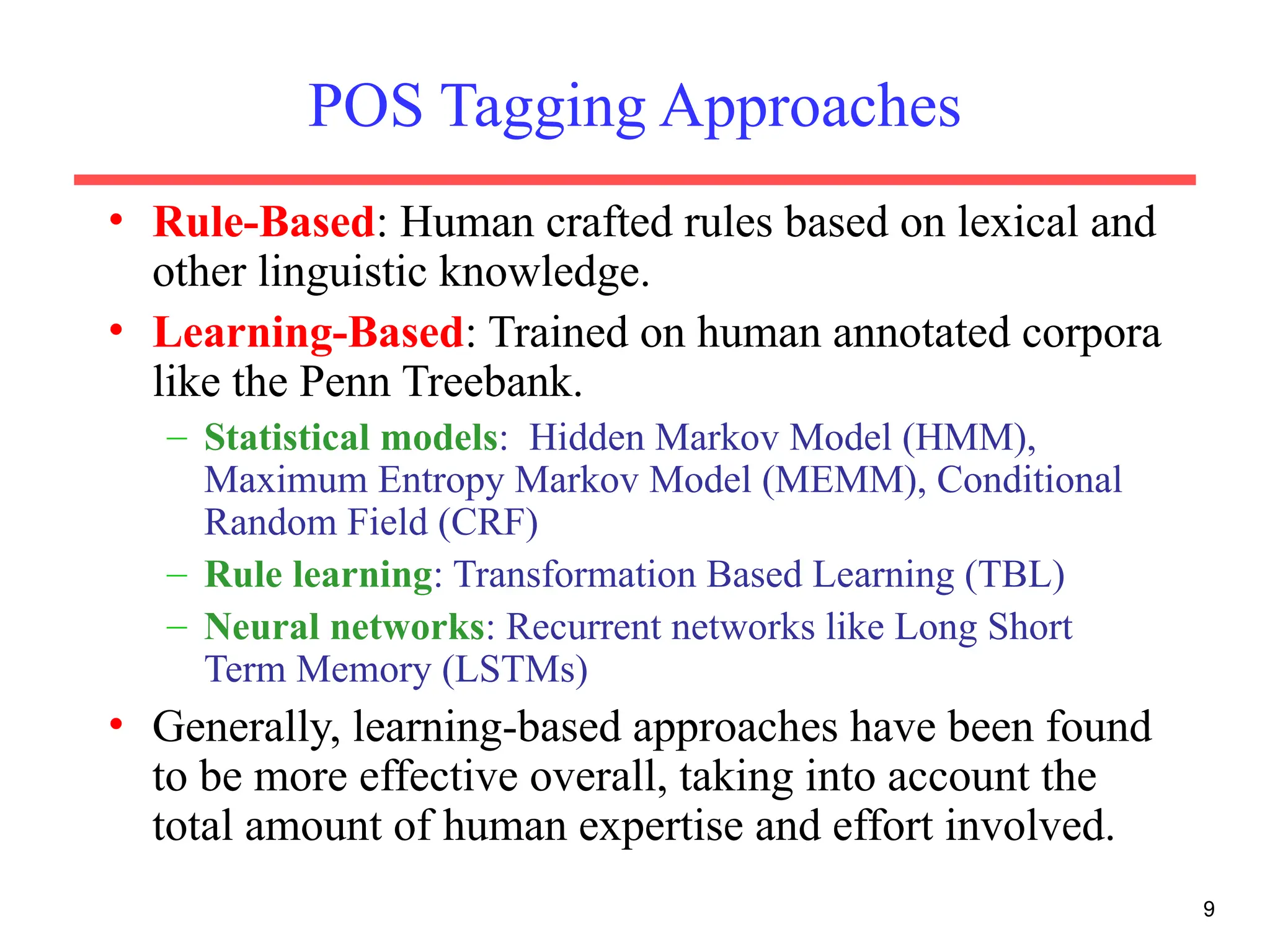
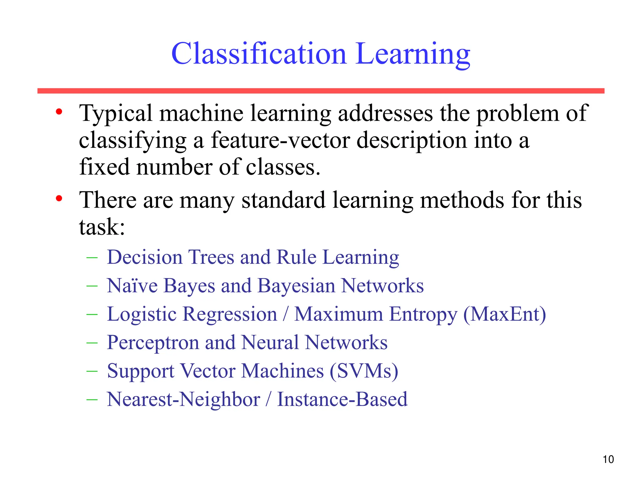
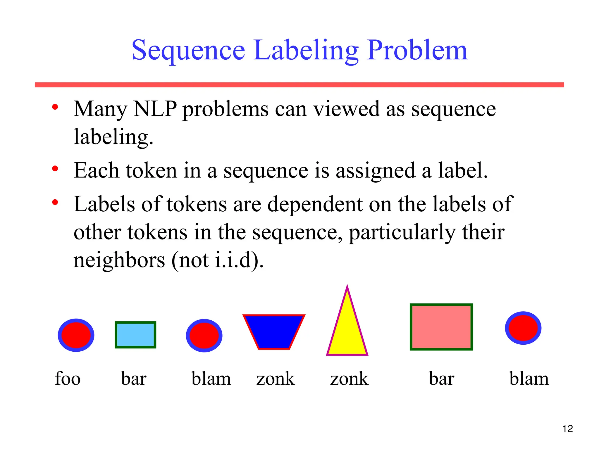
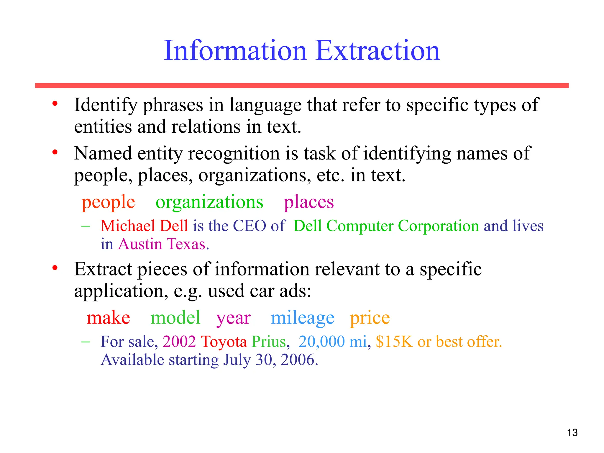
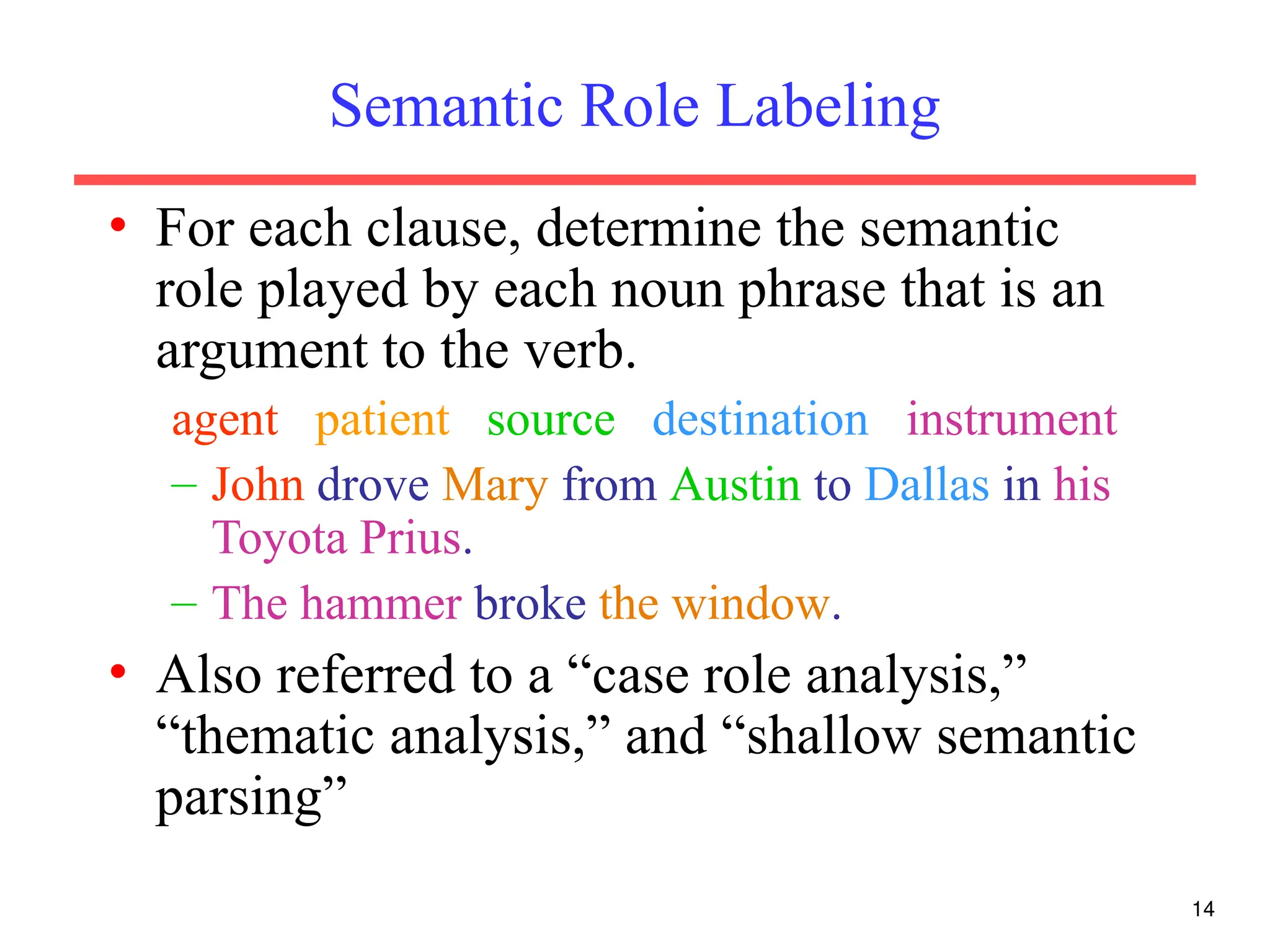
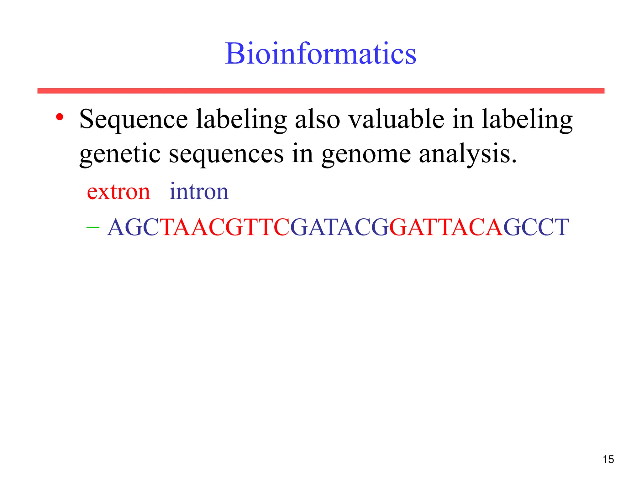
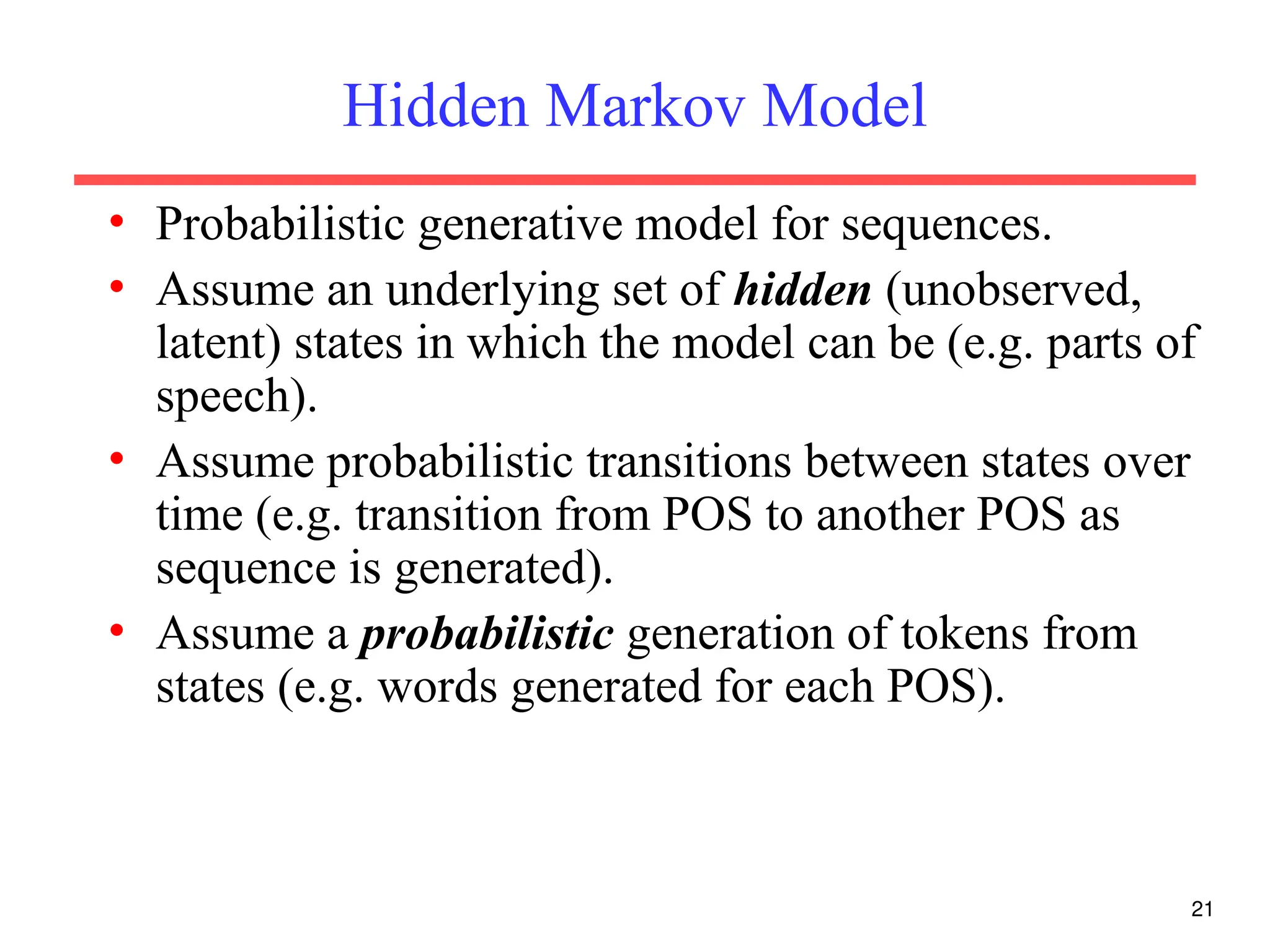
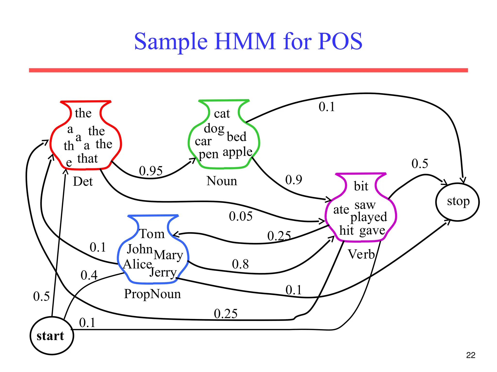
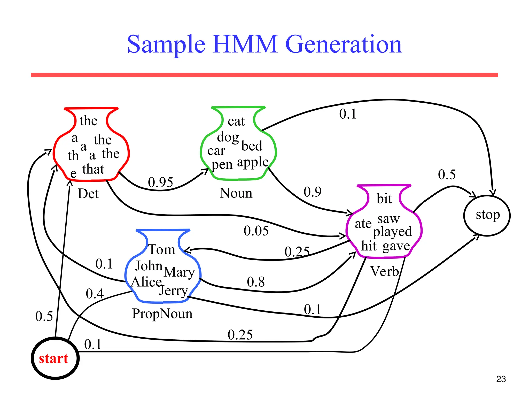
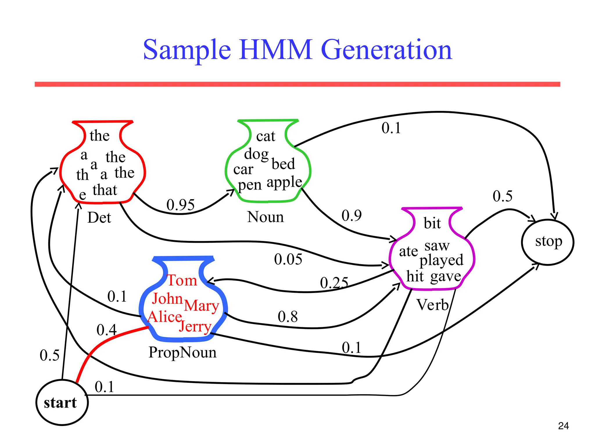
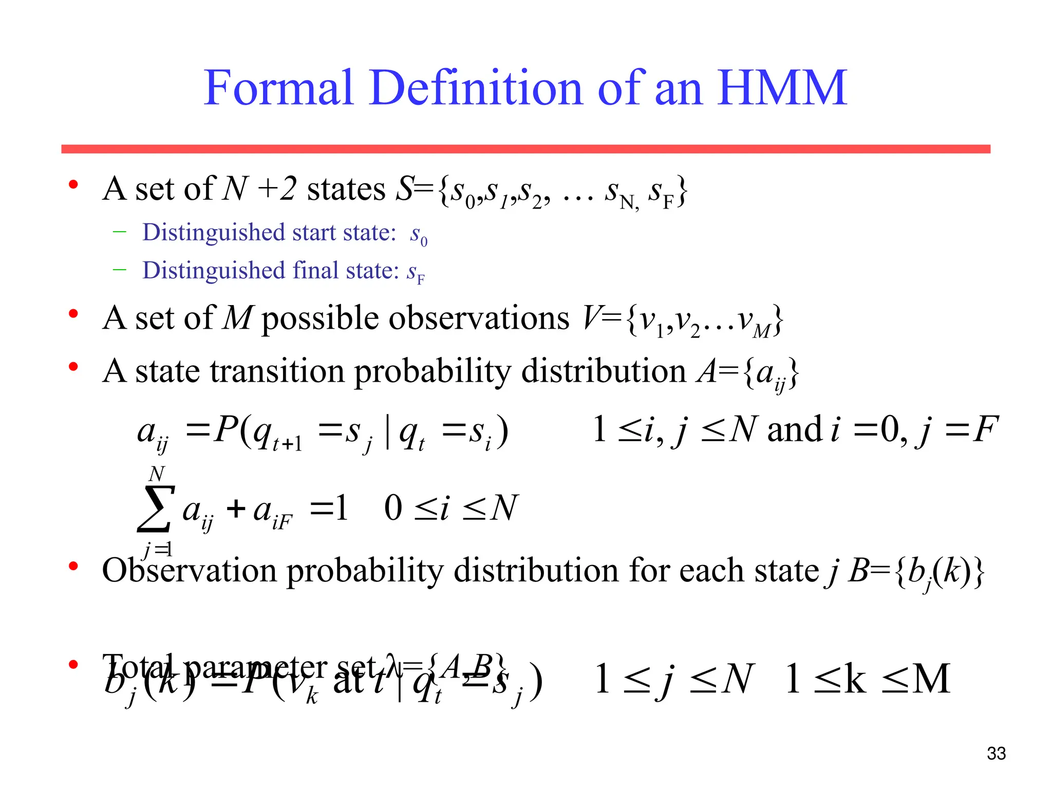
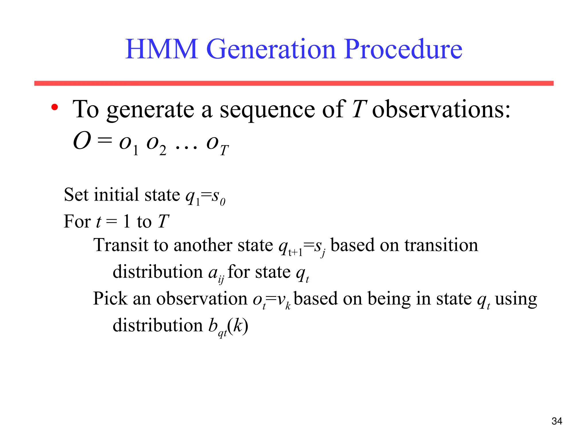
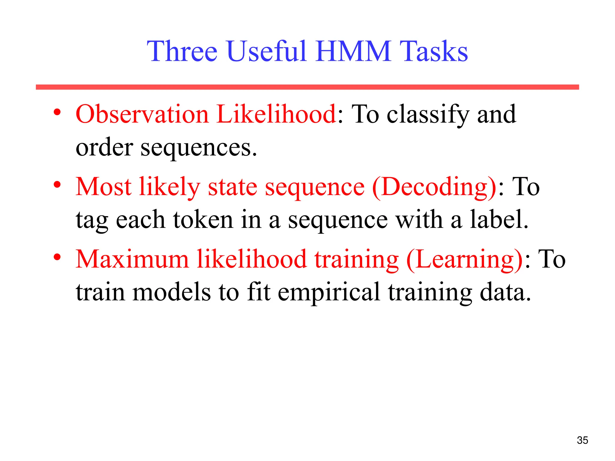
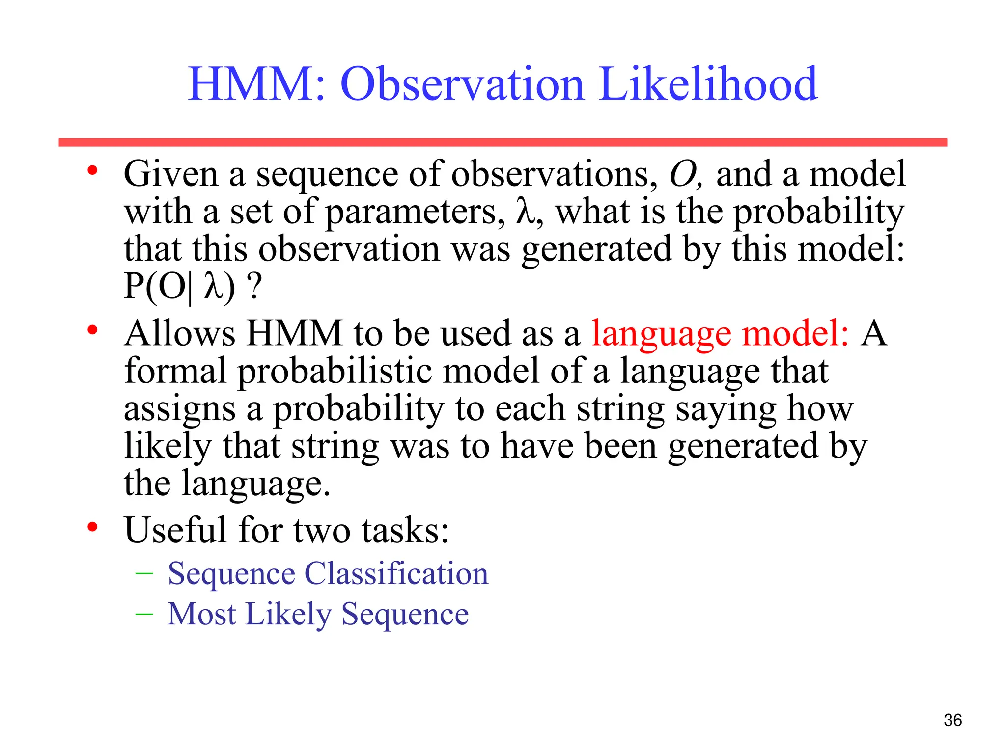
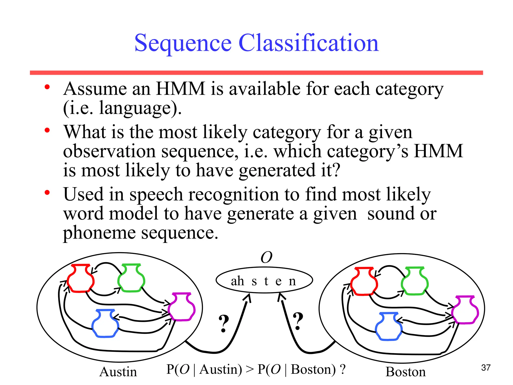
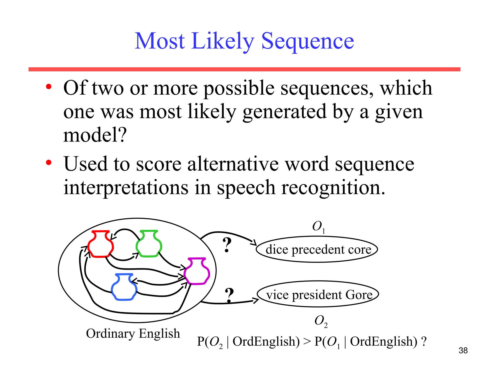
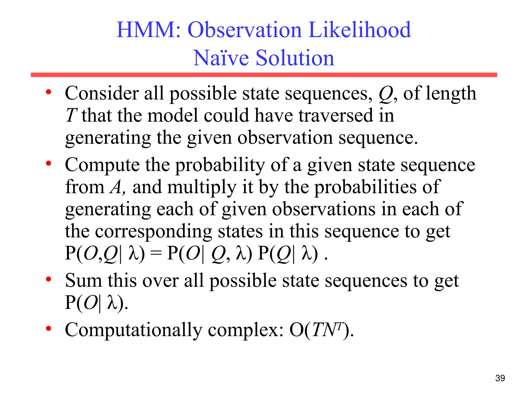
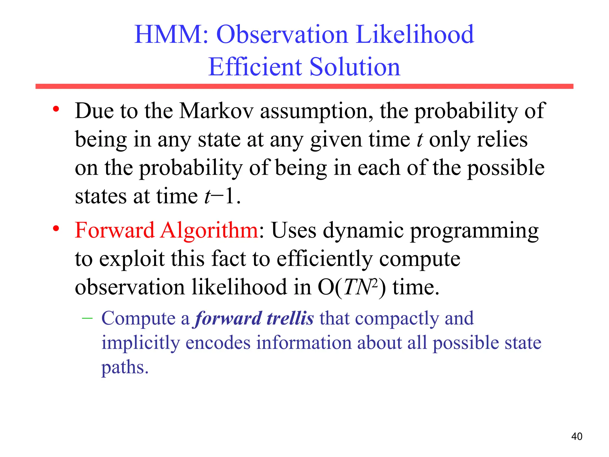
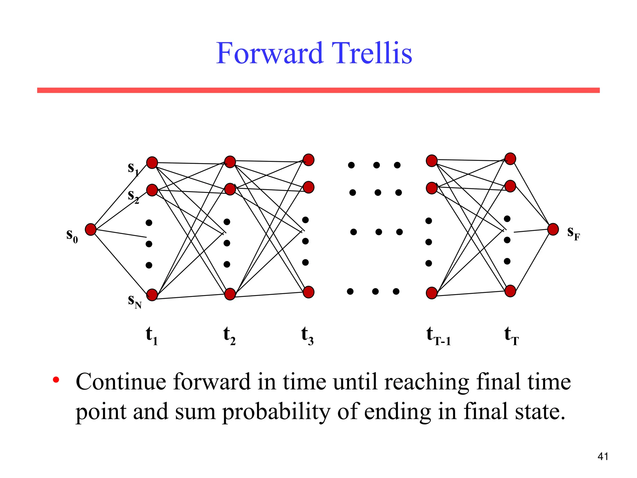
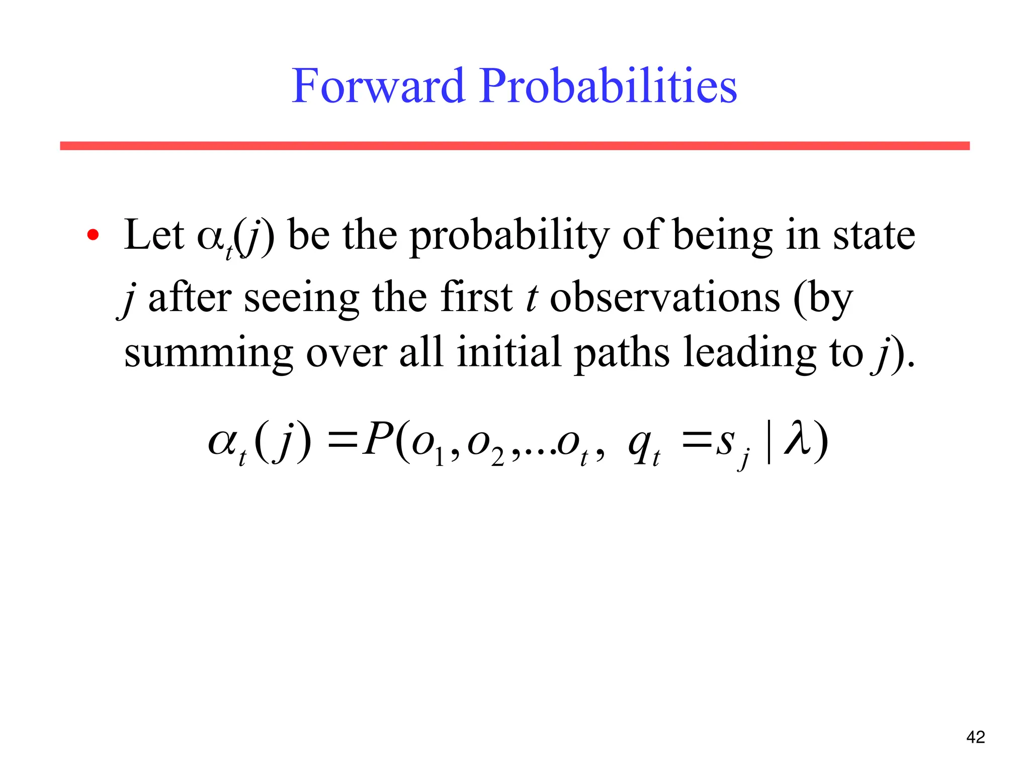
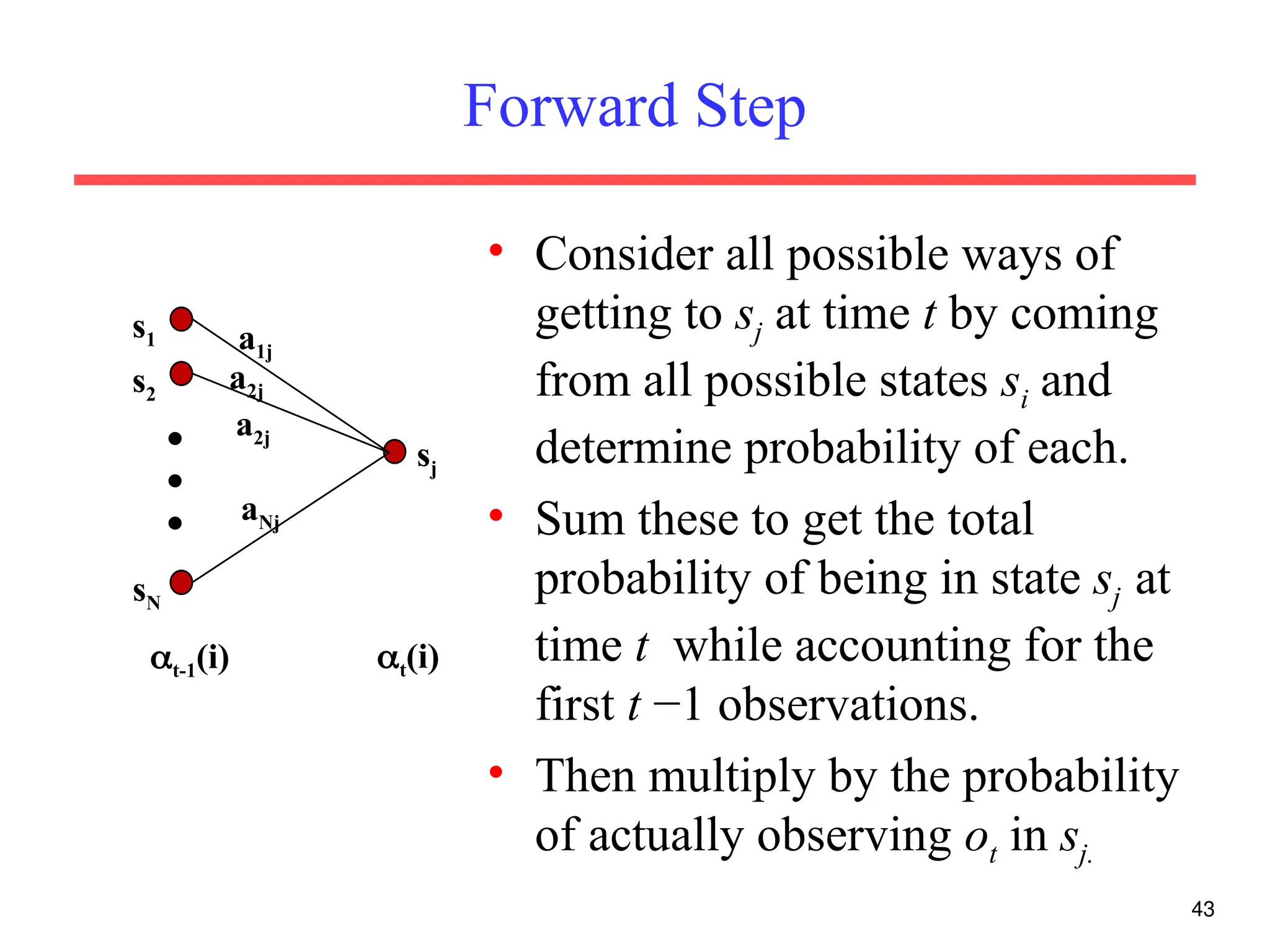
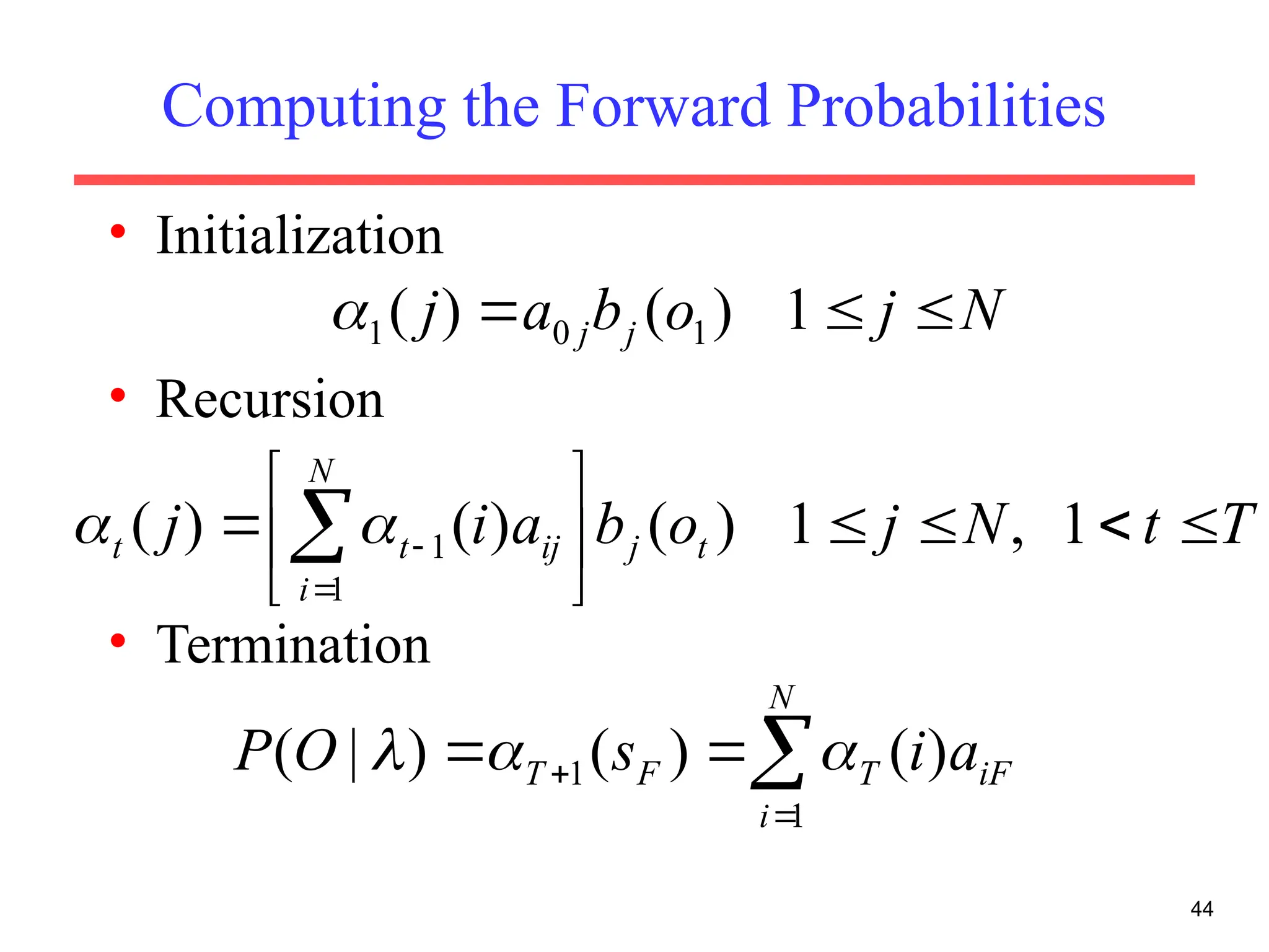
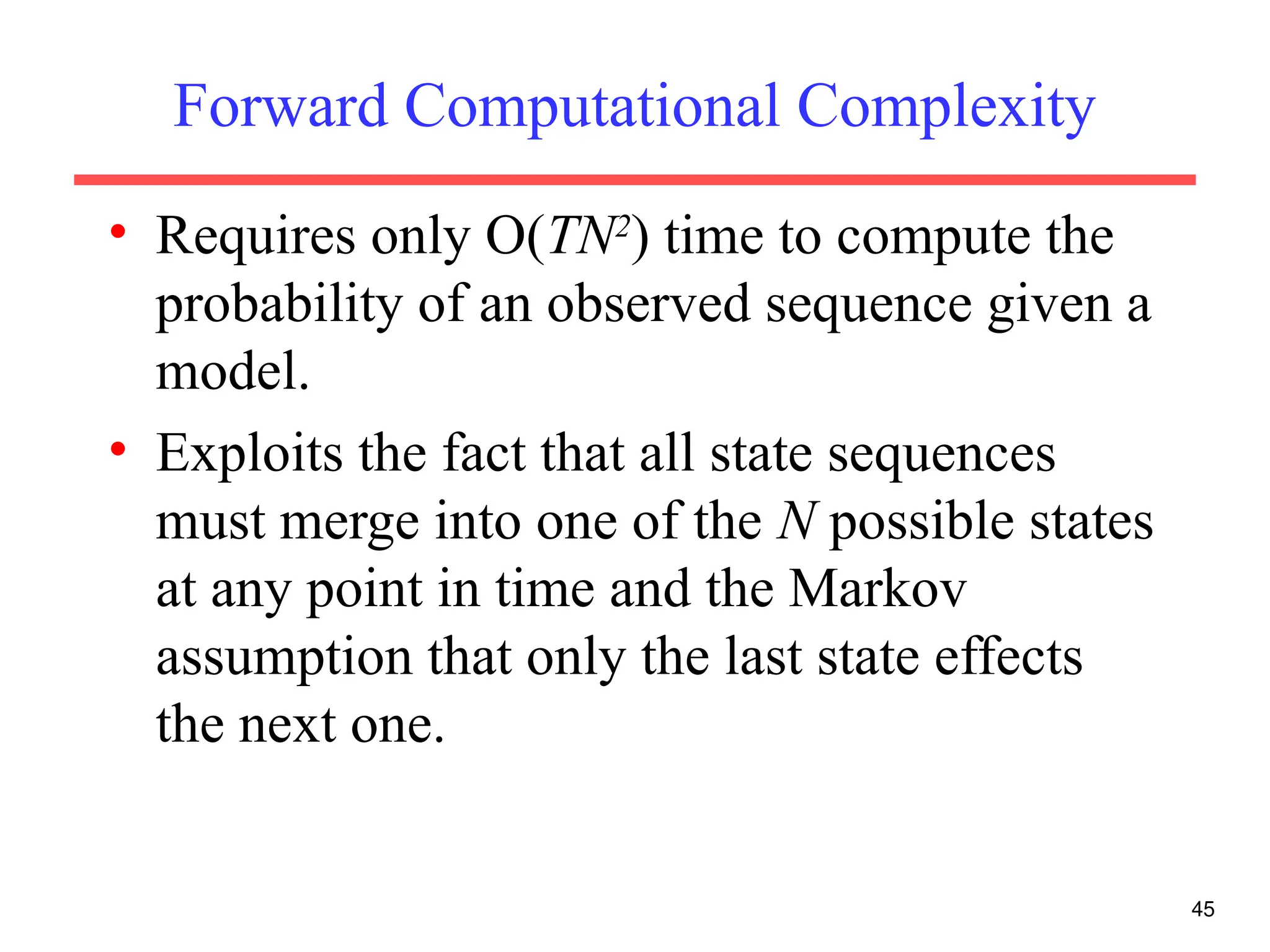
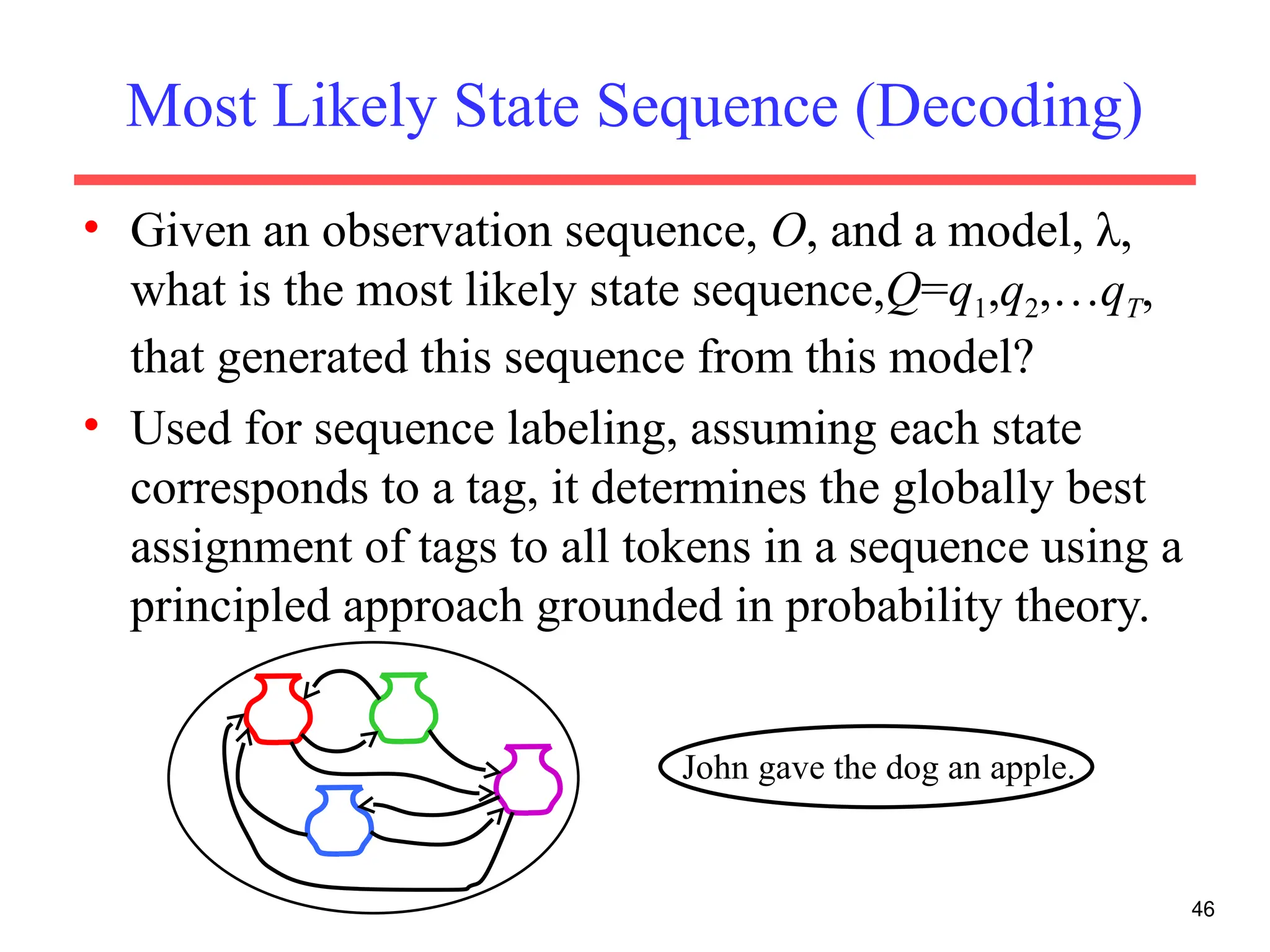
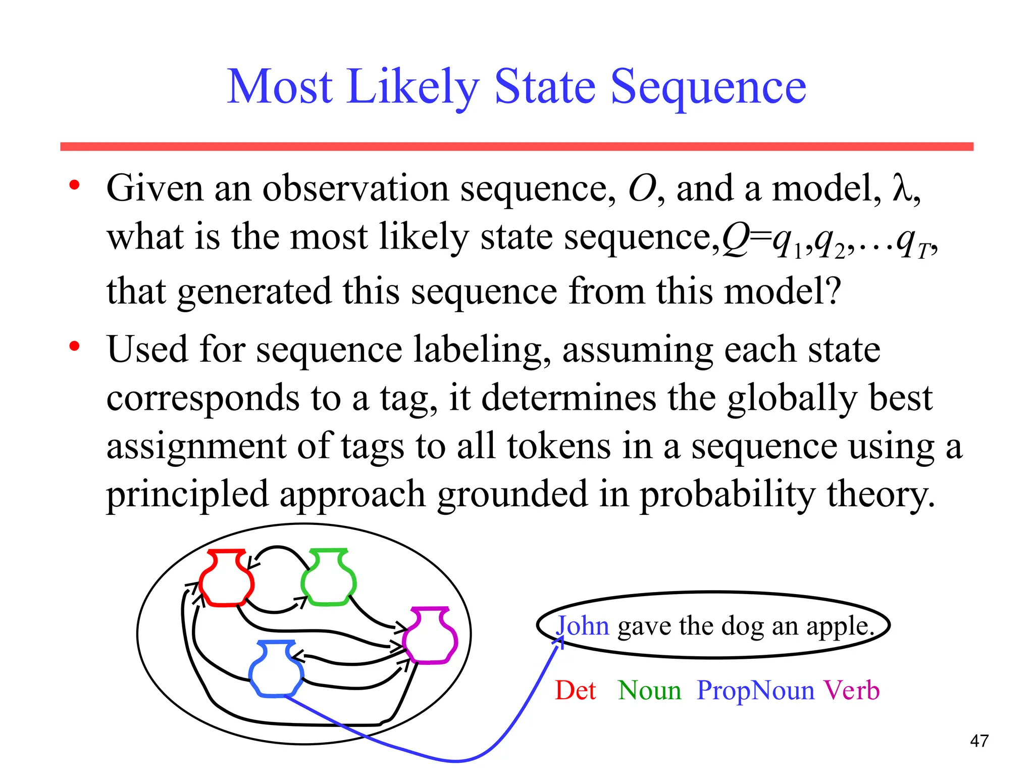
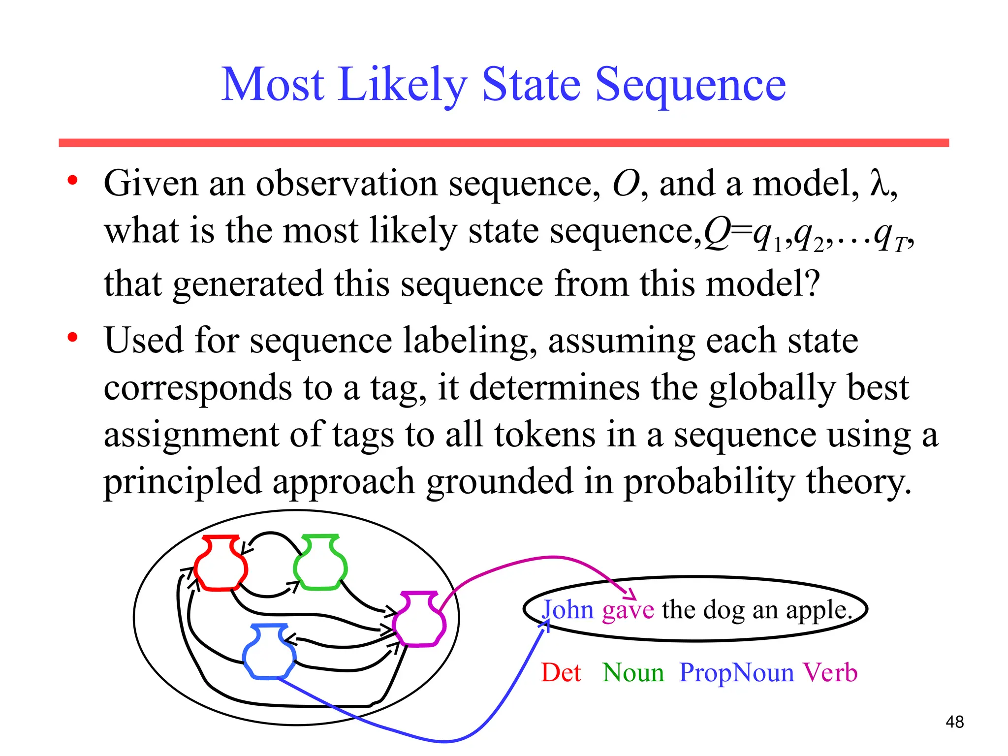
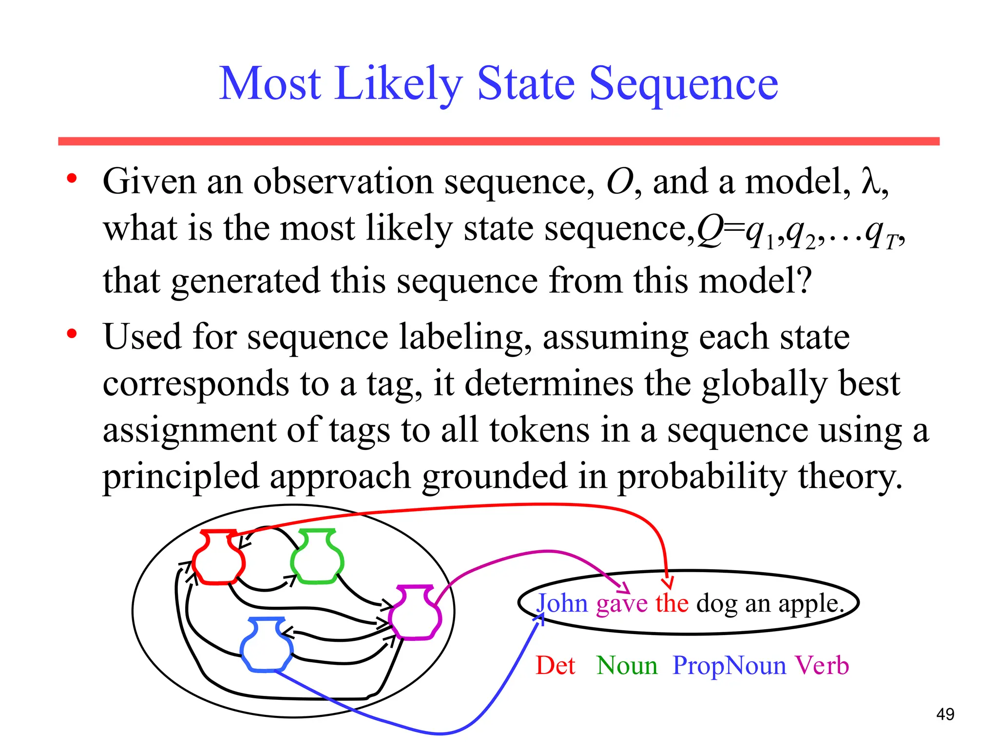
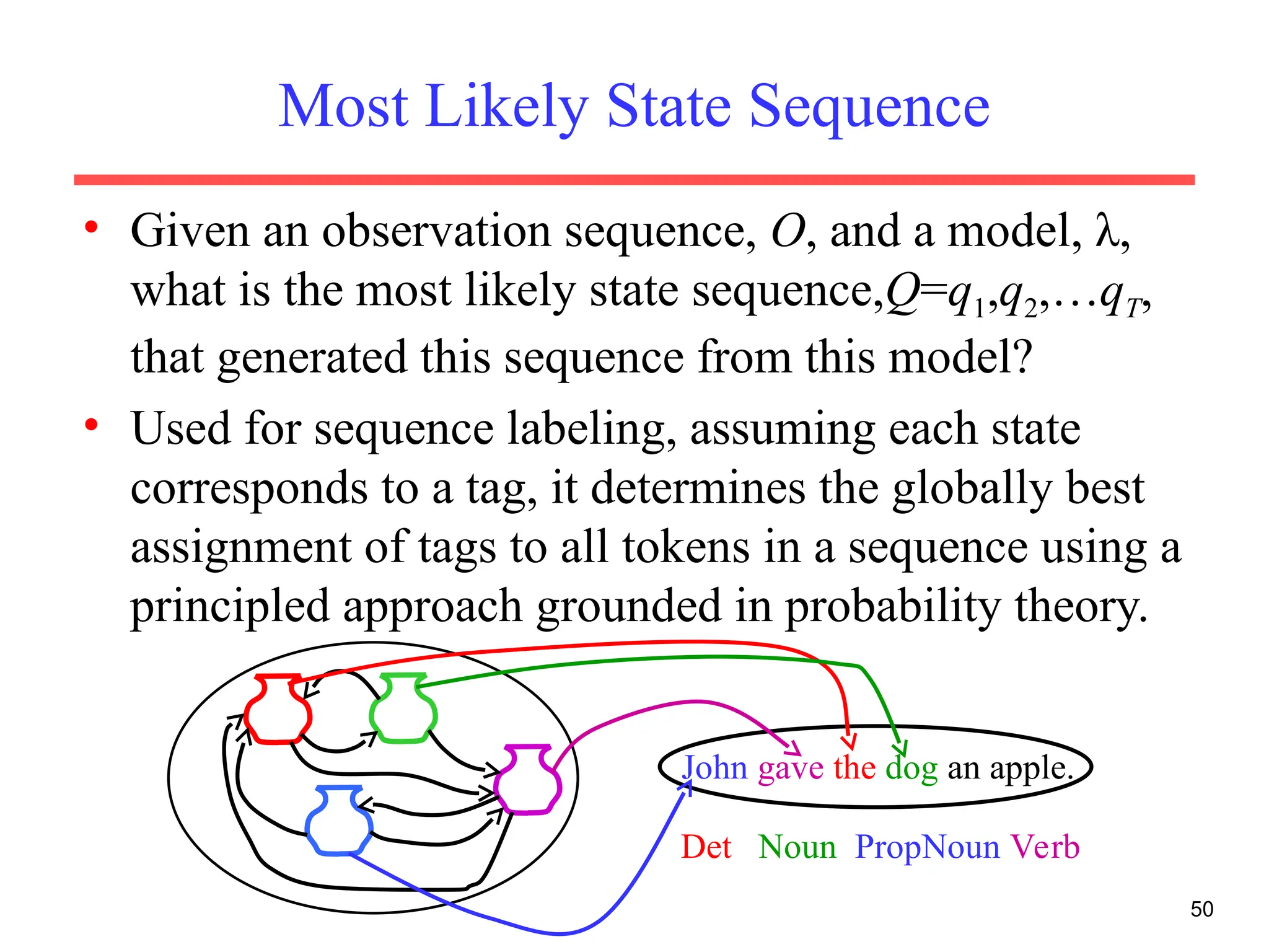
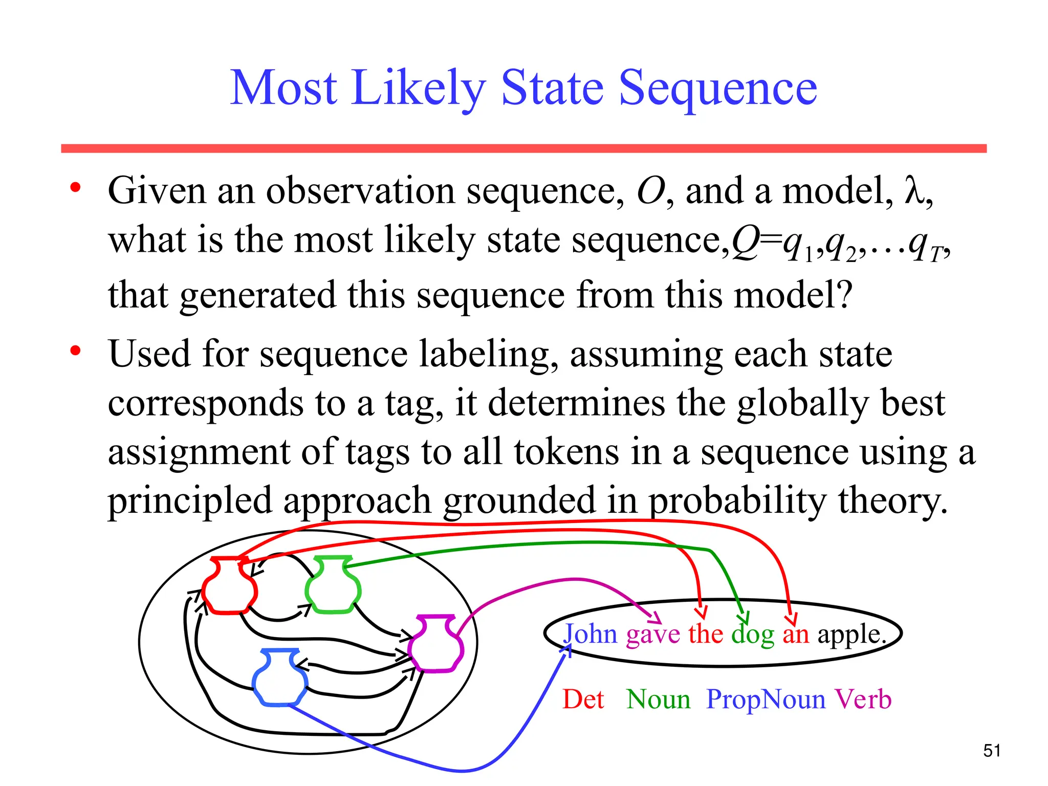
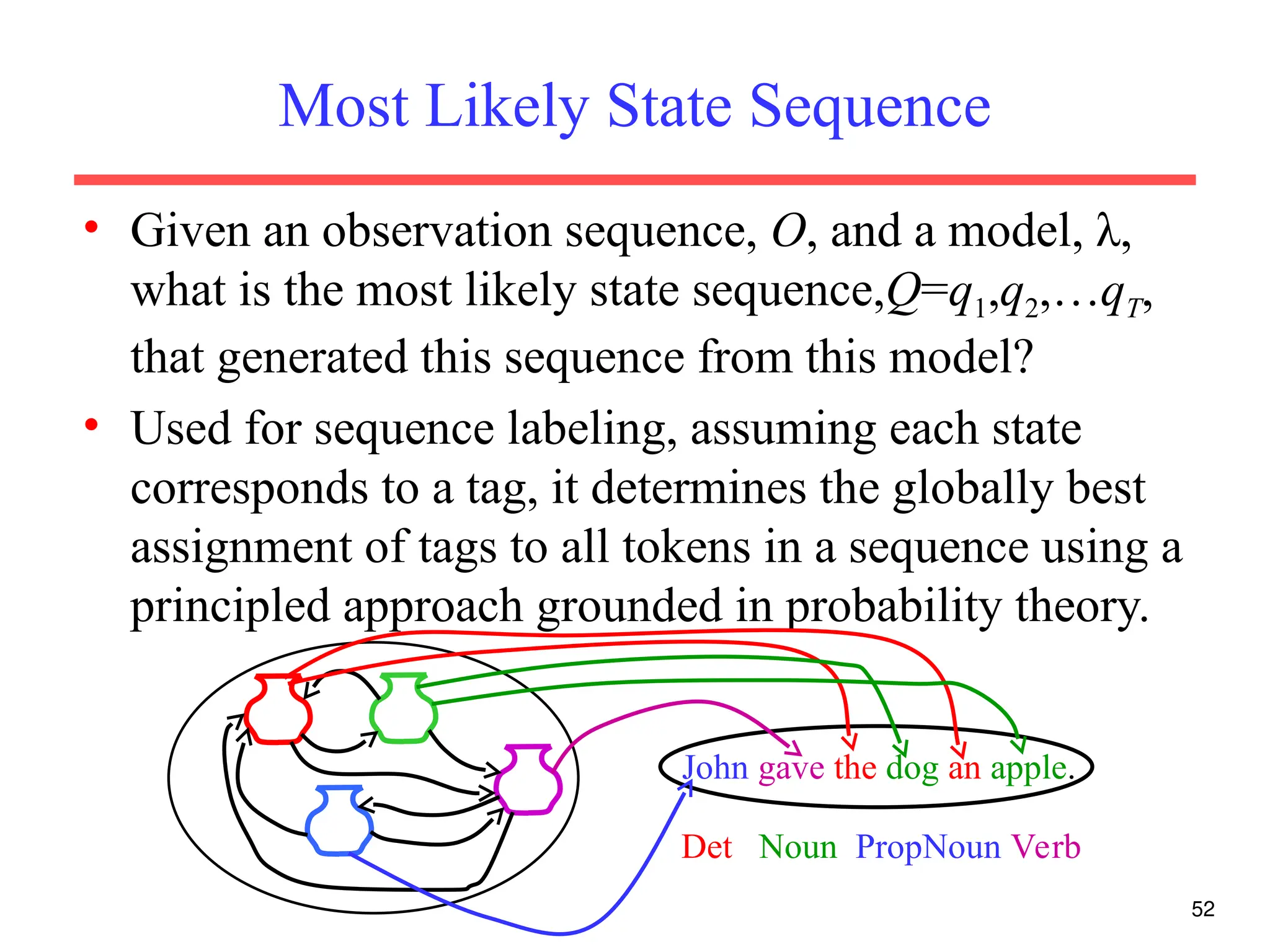
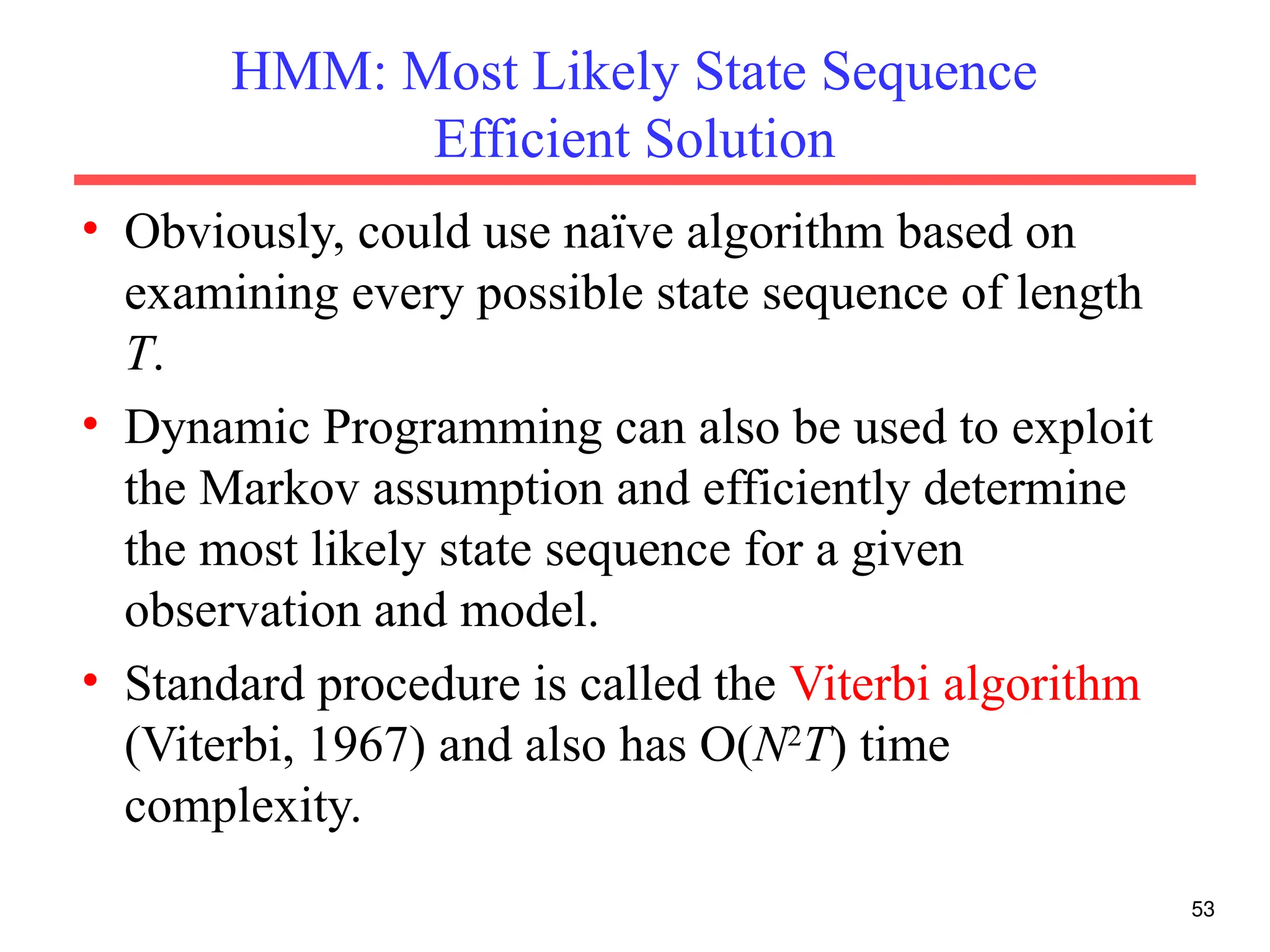
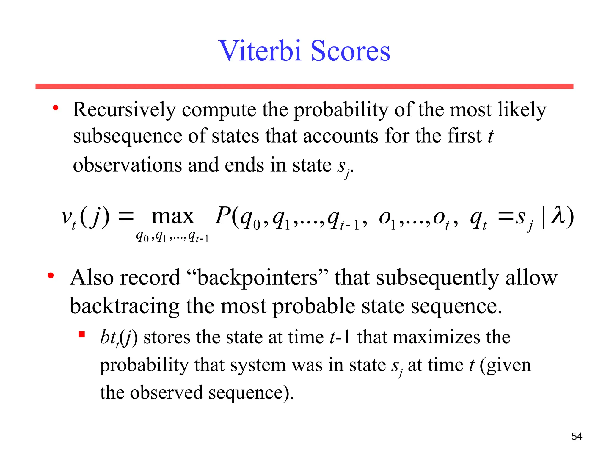
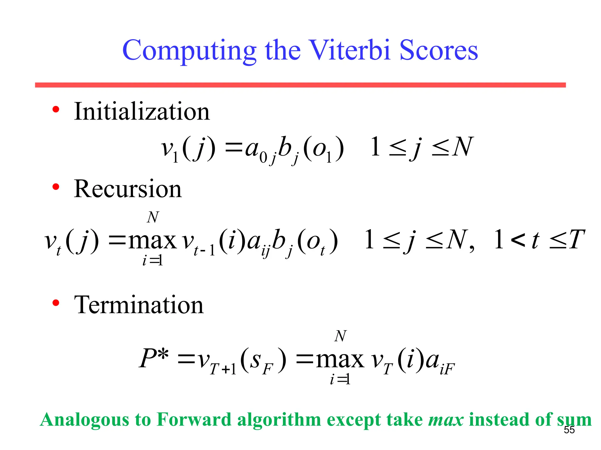
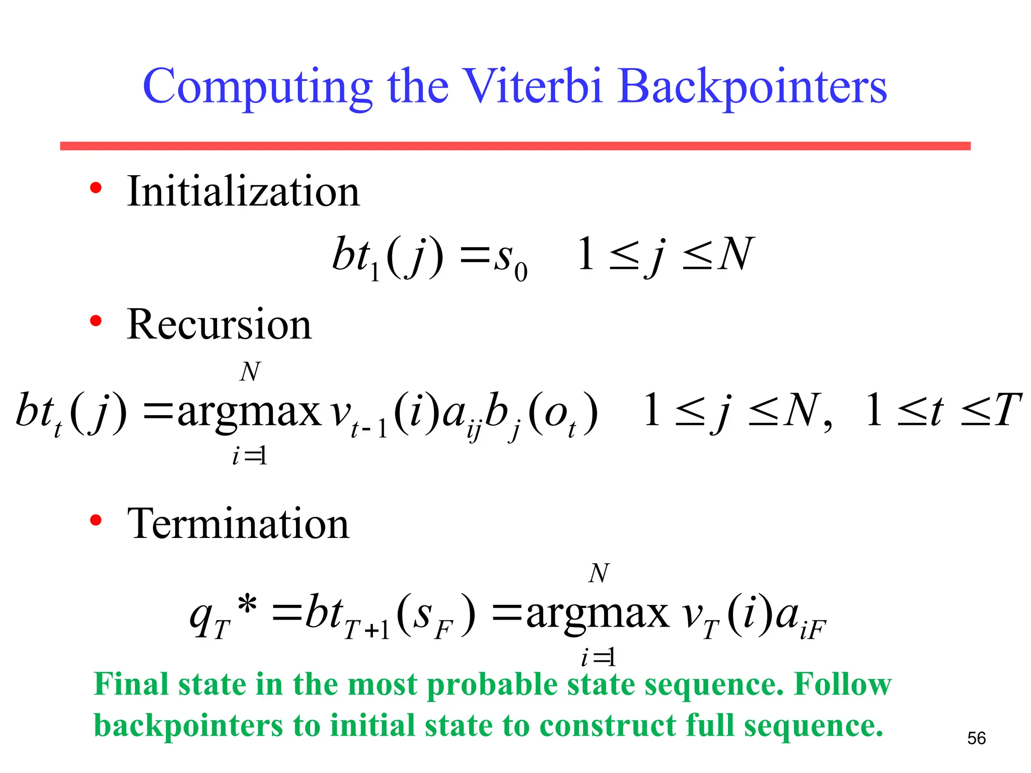
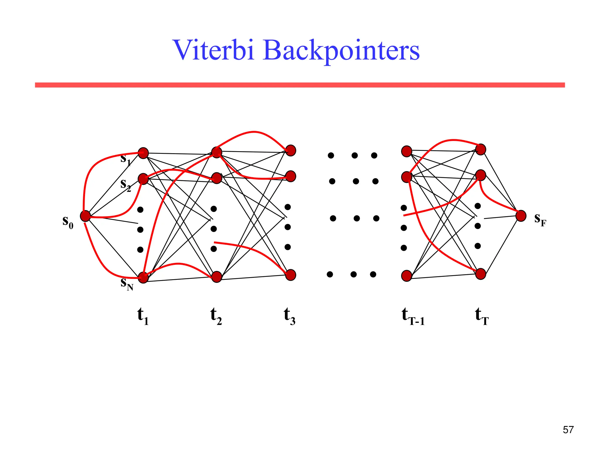
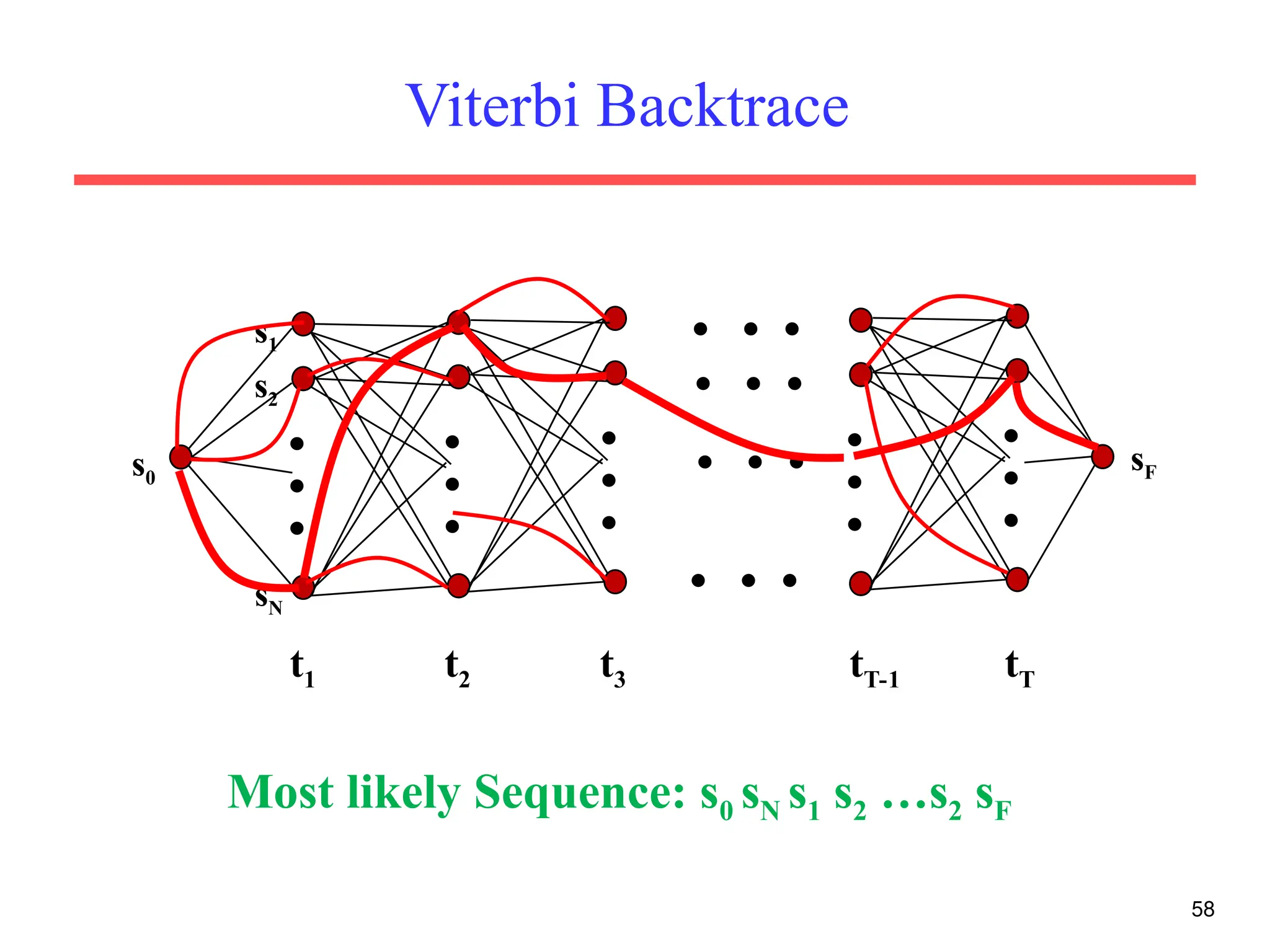
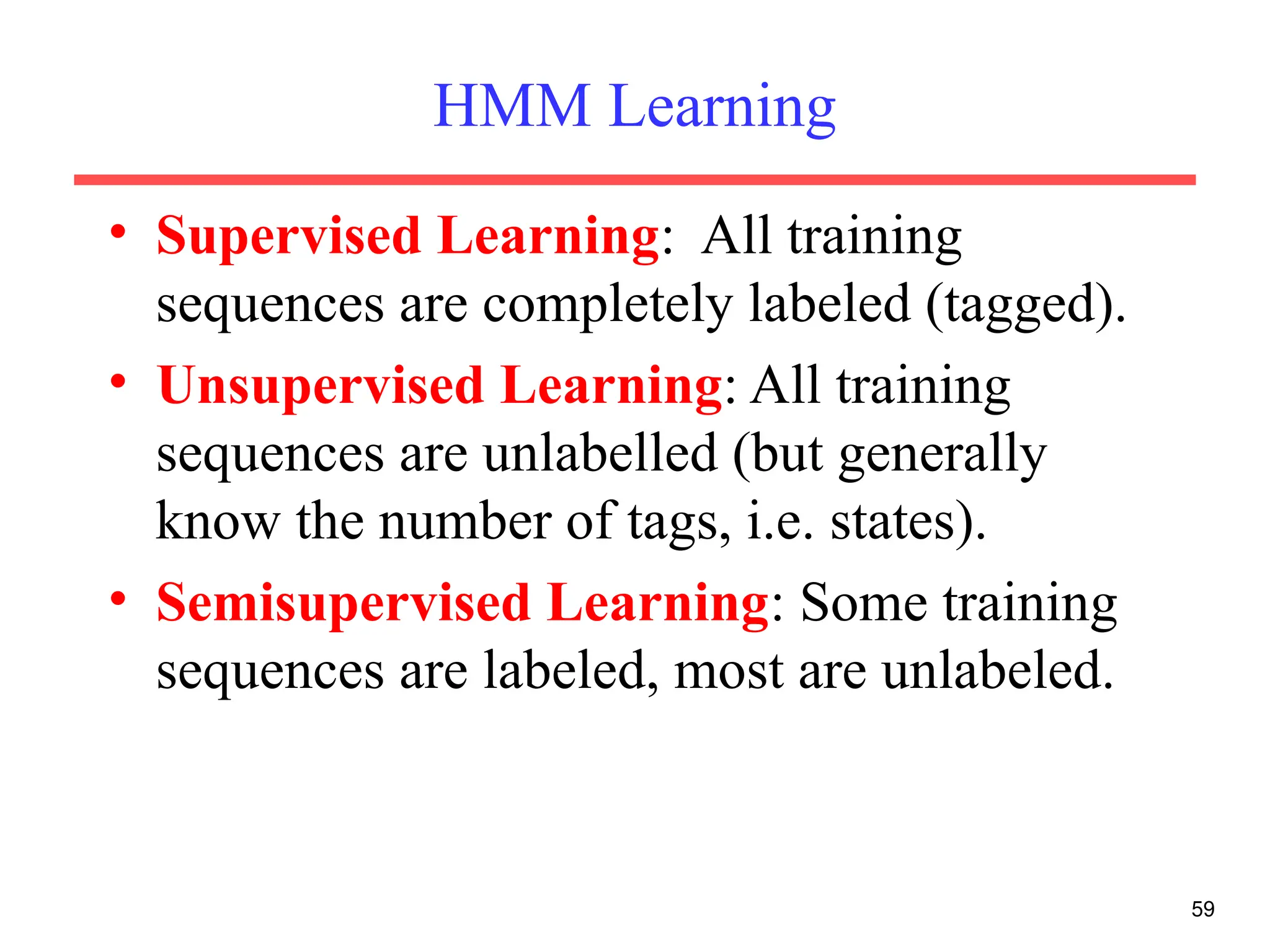
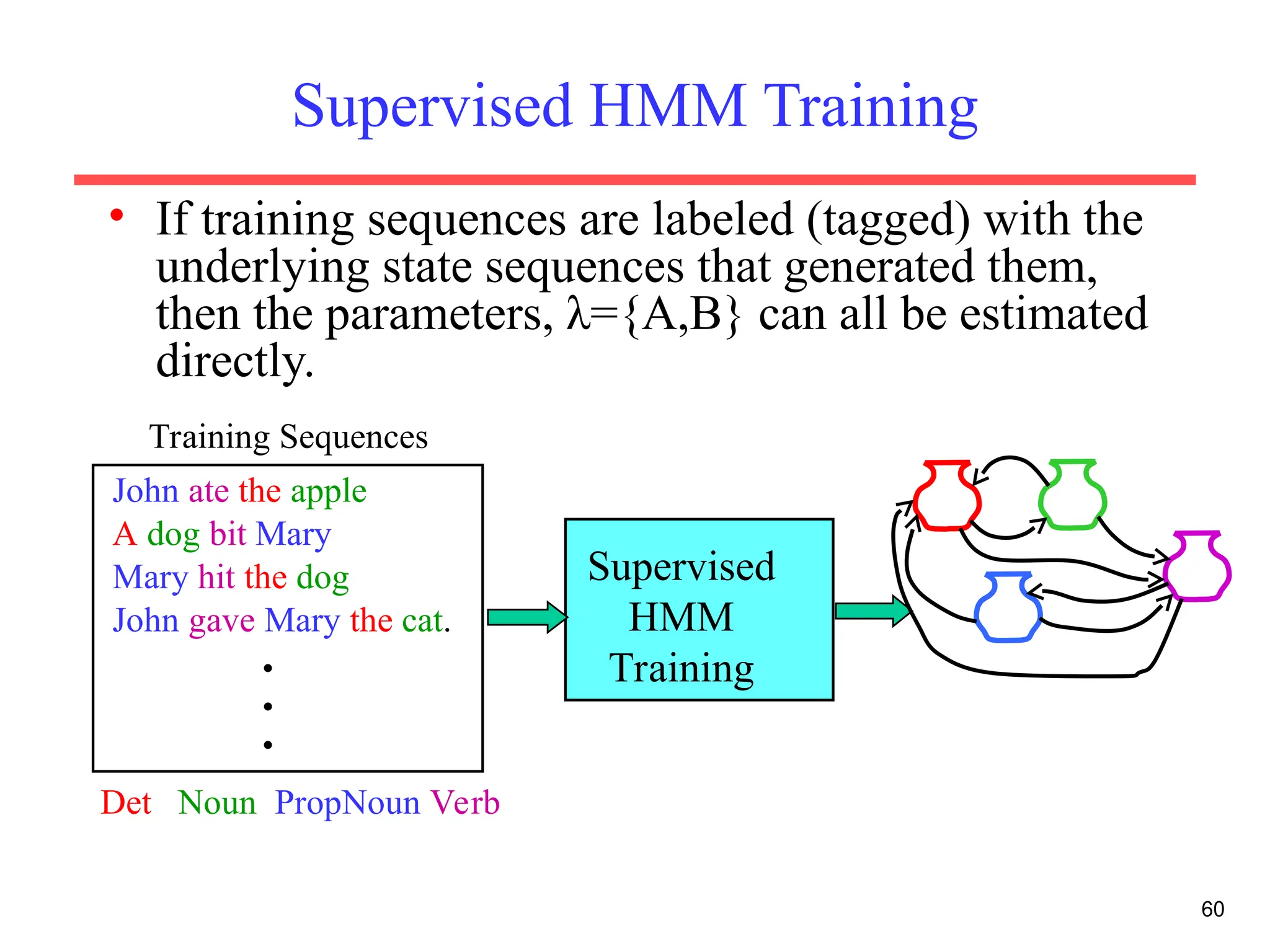
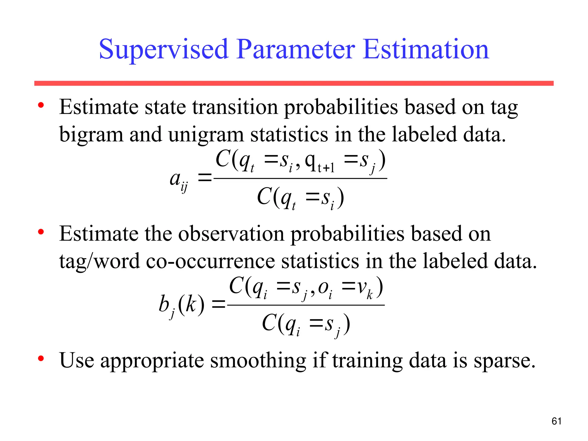
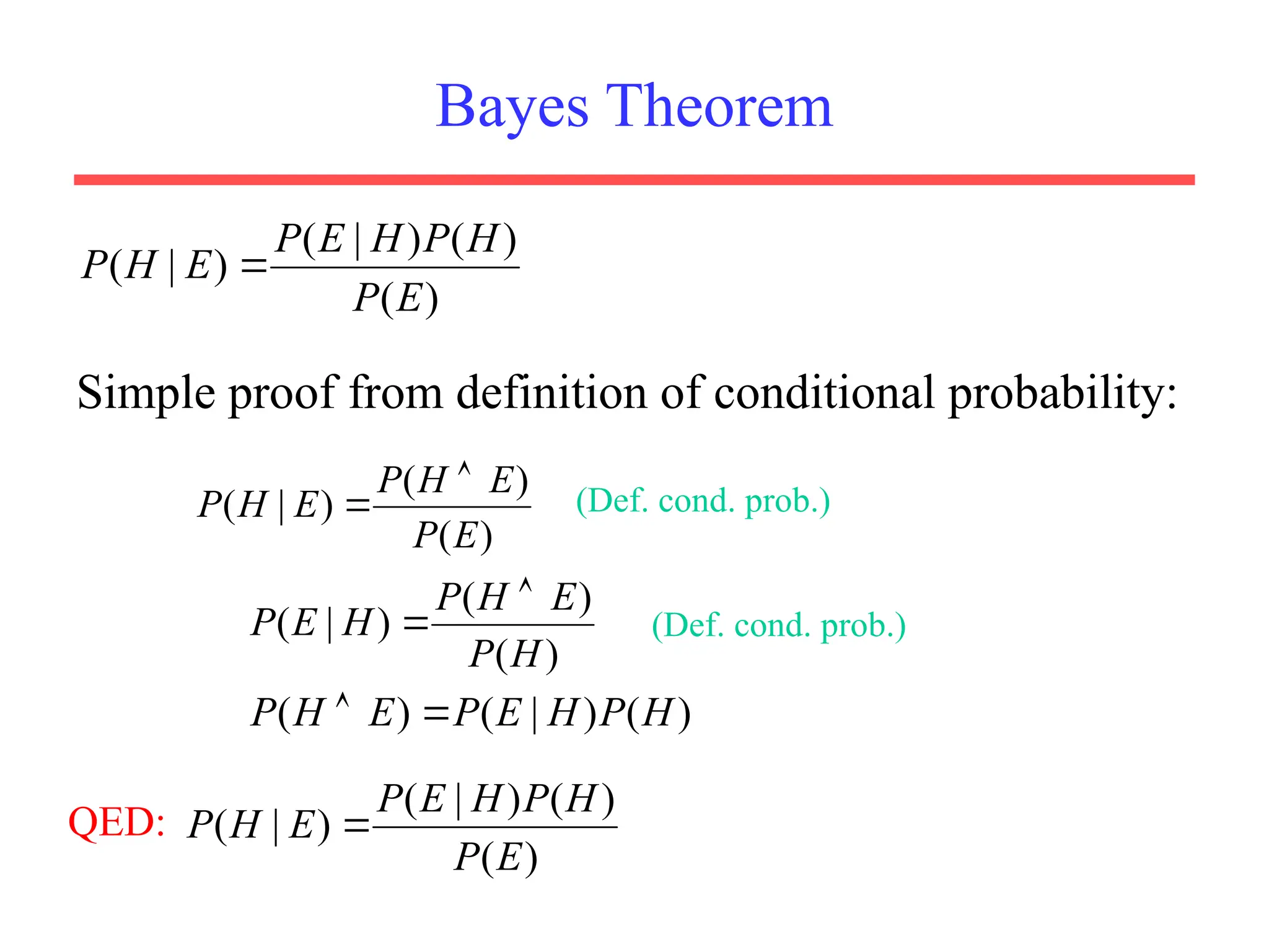
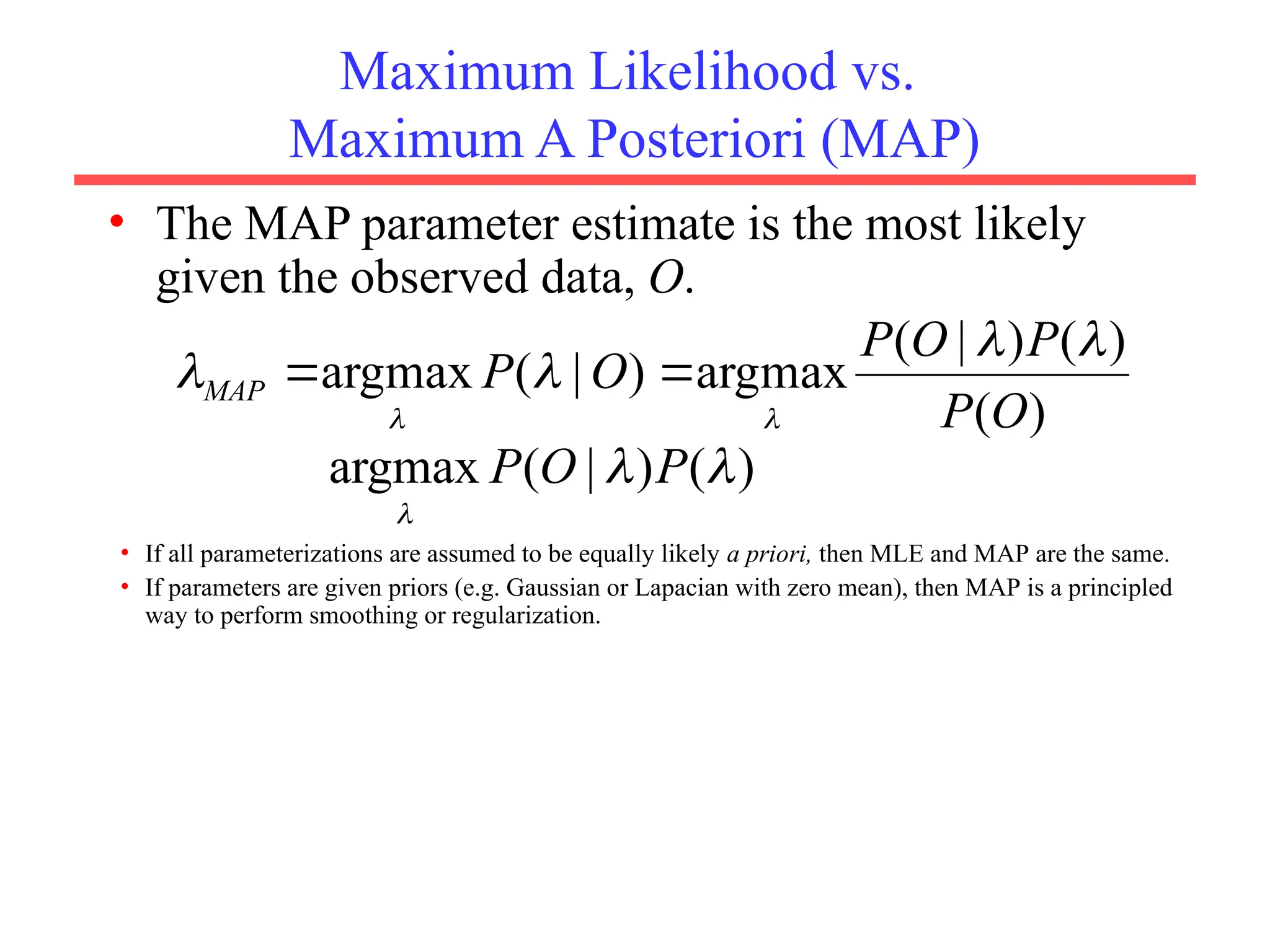
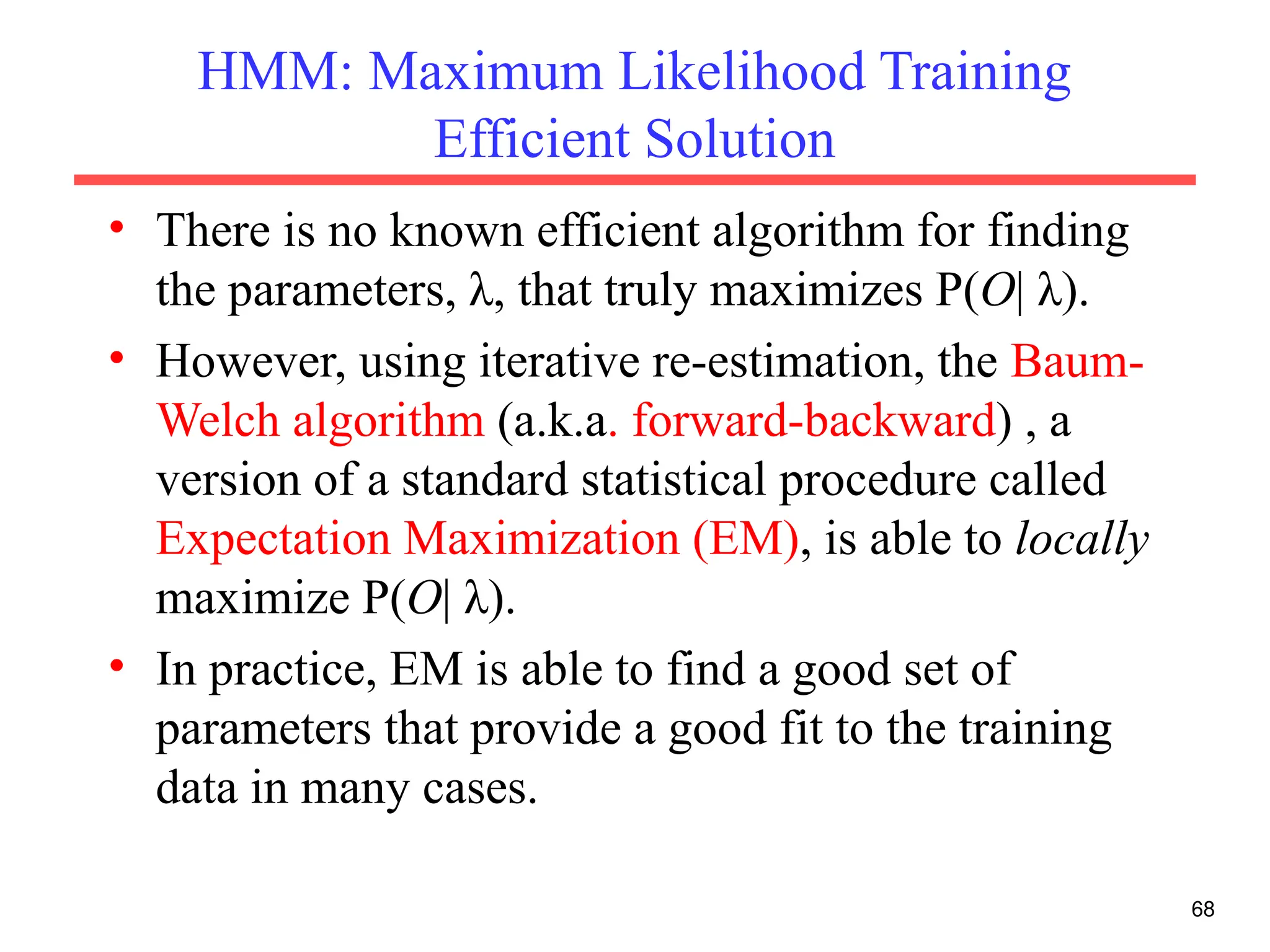
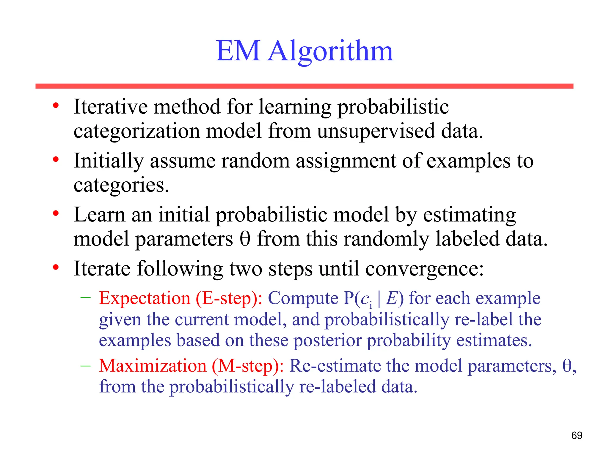
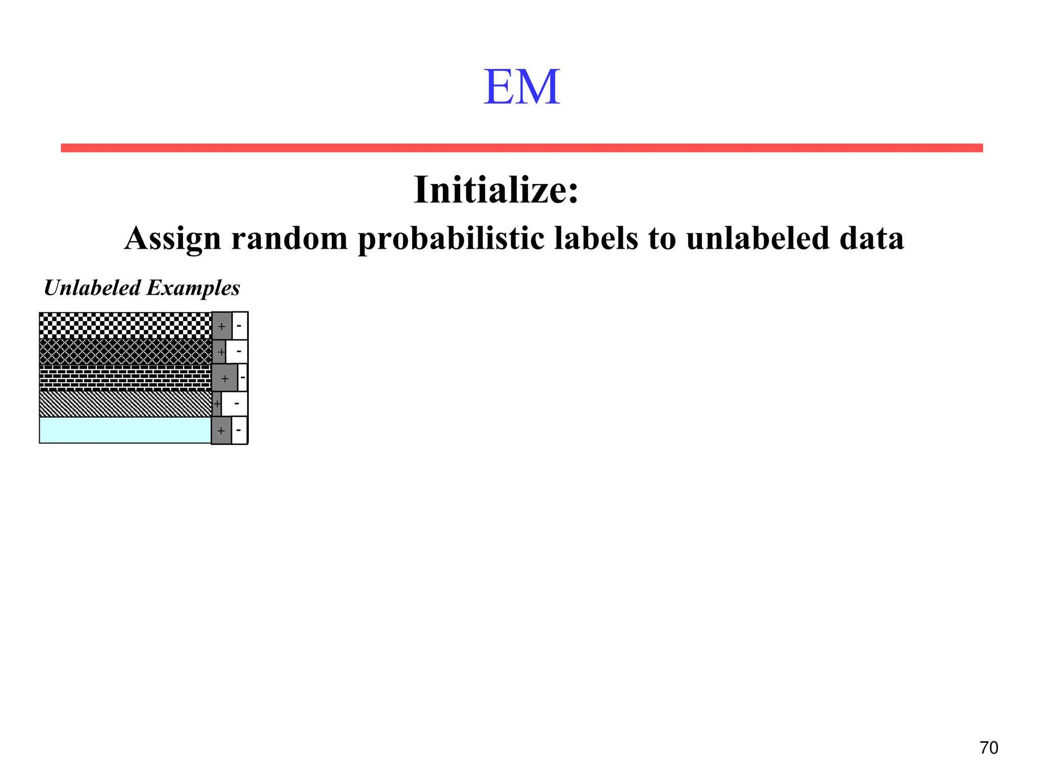
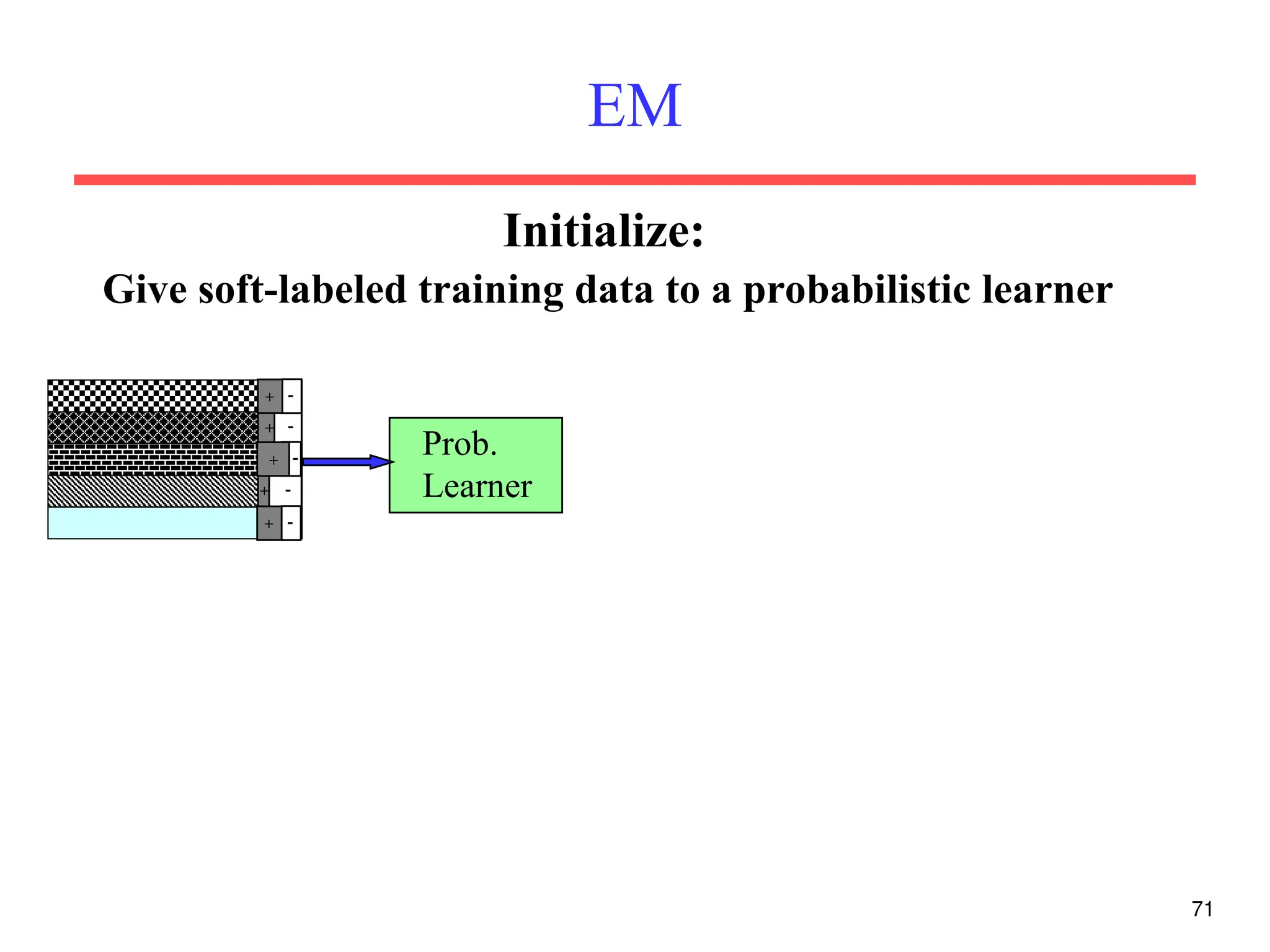
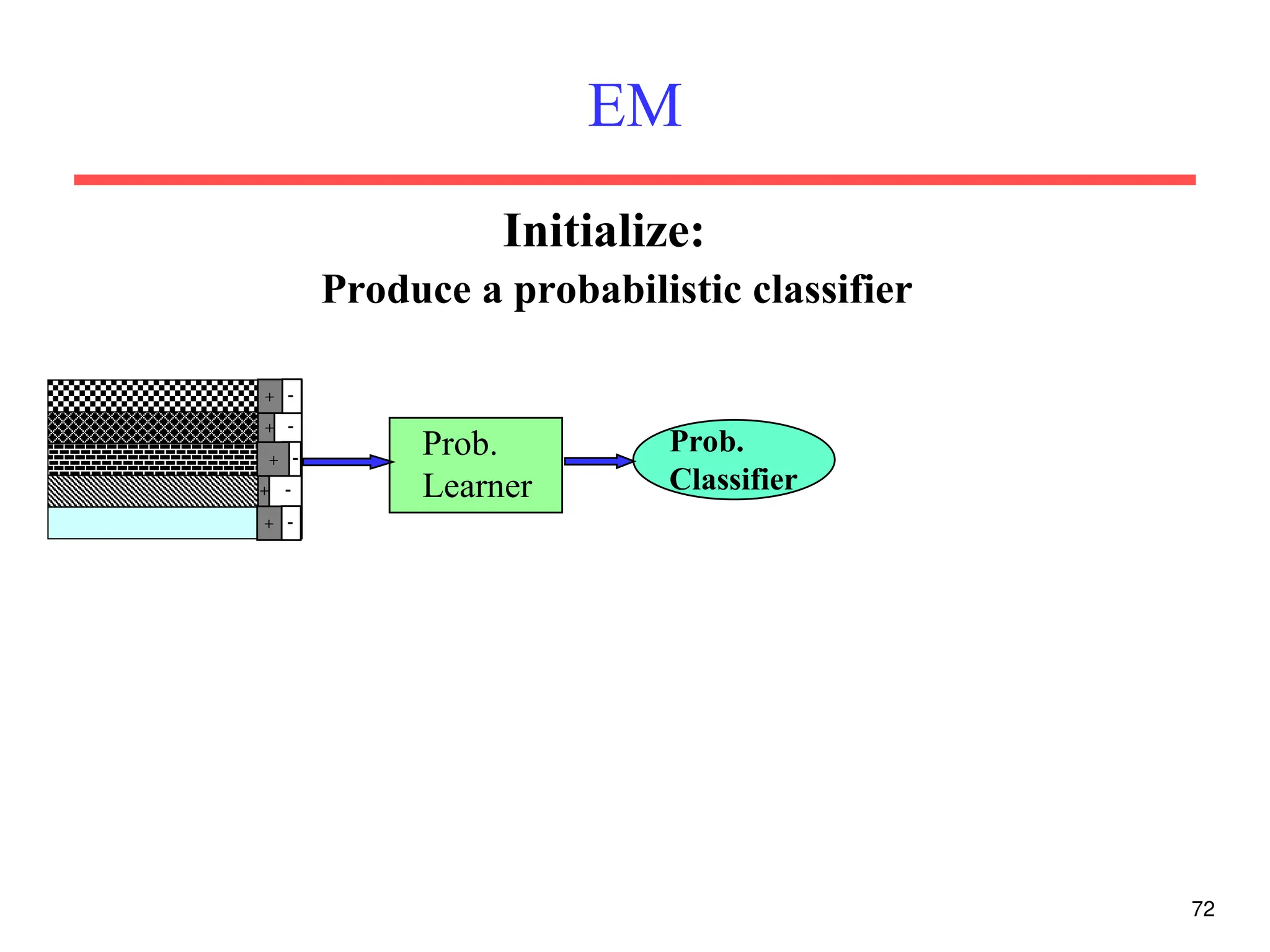
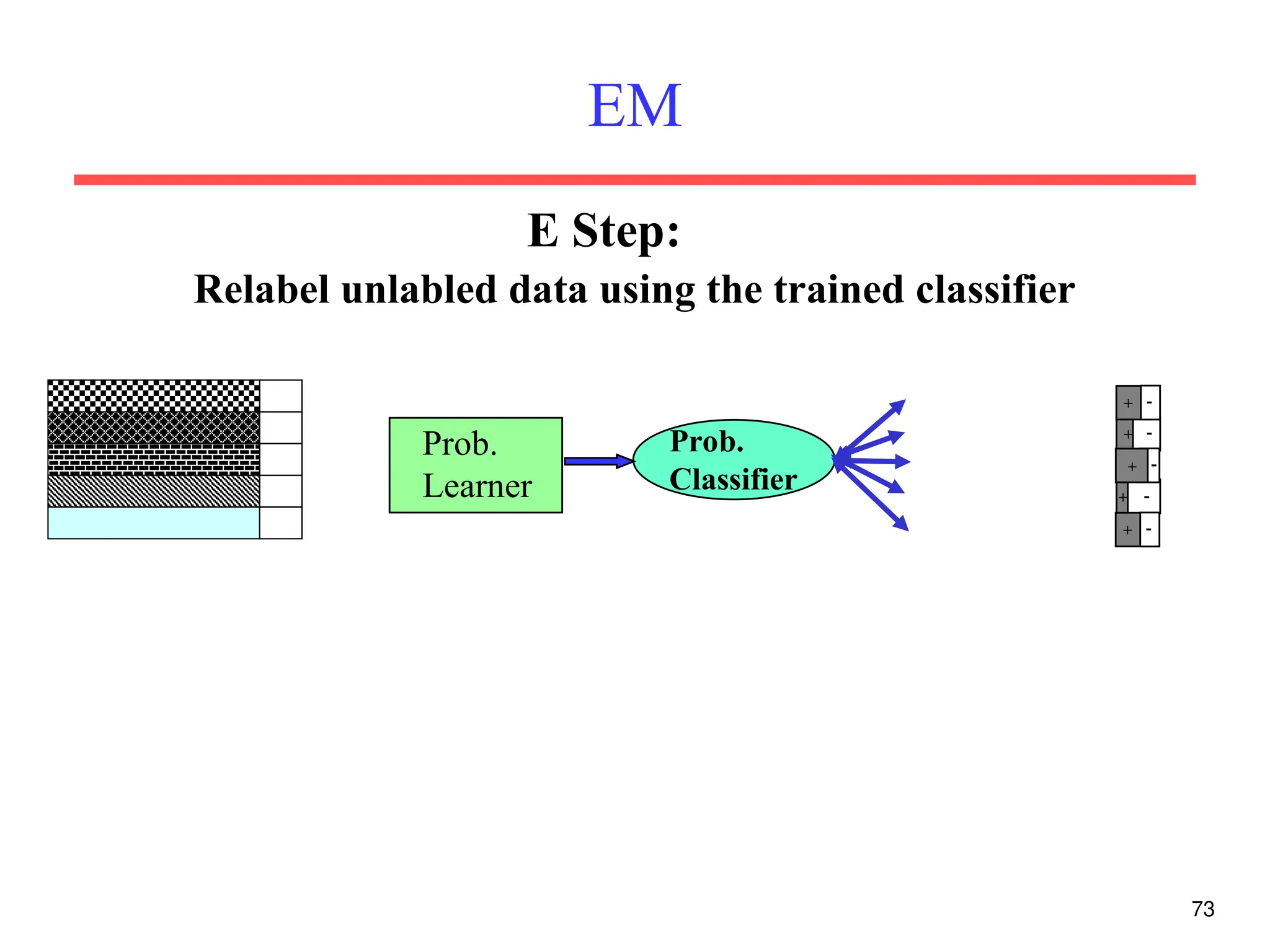
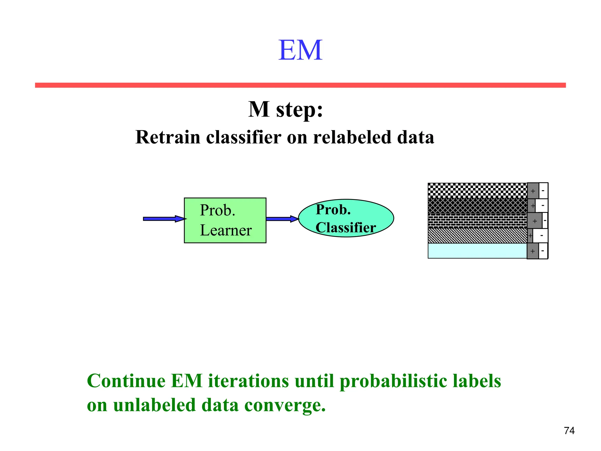
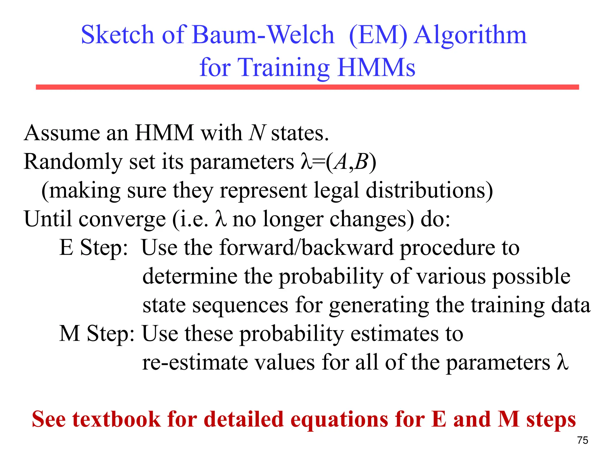
1
1
CS 388:
Natural Language Processing:
Part-Of-Speech Tagging,
Sequence Labeling, and
Hidden Markov Models (HMMs)
Raymond J. Mooney
University of Texas at Austin
2
Part Of Speech Tagging
• Annotate each word in a sentence with a
part-of-speech marker.
• Lowest level of syntactic analysis.
• Useful for subsequent syntactic parsing and
word sense disambiguation.
John saw the saw and decided to take it to the table.
NNP VBD DT NN CC VBD TO VB PRP IN DT NN
3
English POS Tagsets
• Original Brown corpus used a large set of
87 POS tags.
• Most common in NLP today is the Penn
Treebank set of 45 tags.
– Tagset used in these slides.
– Reduced from the Brown set for use in the
context of a parsed corpus (i.e. treebank).
• The C5 tagset used for the British National
Corpus (BNC) has 61 tags.
4
English Parts of Speech
• Noun (person, place or thing)
– Singular (NN): dog, fork
– Plural (NNS): dogs, forks
– Proper (NNP, NNPS): John, Springfields
– Personal pronoun (PRP): I, you, he, she, it
– Wh-pronoun (WP): who, what
• Verb (actions and processes)
– Base, infinitive (VB): eat
– Past tense (VBD): ate
– Gerund (VBG): eating
– Past participle (VBN): eaten
– Non 3rd
person singular present tense (VBP): eat
– 3rd
person singular present tense: (VBZ): eats
– Modal (MD): should, can
– To (TO): to (to eat)
5
English Parts of Speech (cont.)
• Adjective (modify nouns)
– Basic (JJ): red, tall
– Comparative (JJR): redder, taller
– Superlative (JJS): reddest, tallest
• Adverb (modify verbs)
– Basic (RB): quickly
– Comparative (RBR): quicker
– Superlative (RBS): quickest
• Preposition (IN): on, in, by, to, with
• Determiner:
– Basic (DT) a, an, the
– WH-determiner (WDT): which, that
• Coordinating Conjunction (CC): and, but, or,
• Particle (RP): off (took off), up (put up)
Closed vs. Open Class
• Closed class categories are composed of a
small, fixed set of grammatical function
words for a given language.
– Pronouns, Prepositions, Modals, Determiners,
Particles, Conjunctions
• Open class categories have large number of
words and new ones are easily invented.
– Nouns (Googler, textlish), Verbs (Google),
Adjectives (geeky), Abverb (automagically)
6
7
Ambiguity in POS Tagging
• “Like” can be a verb or a preposition
– I like/VBP candy.
– Time flies like/IN an arrow.
• “Around” can be a preposition, particle, or
adverb
– I bought it at the shop around/IN the corner.
– I never got around/RP to getting a car.
– A new Prius costs around/RB $25K.
8
POS Tagging Process
• Usually assume a separate initial tokenization process that
separates and/or disambiguates punctuation, including
detecting sentence boundaries.
• Degree of ambiguity in English (based on Brown corpus)
– 11.5% of word types are ambiguous.
– 40% of word tokens are ambiguous.
• Average POS tagging disagreement amongst expert human
judges for the Penn treebank was 3.5%
– Based on correcting the output of an initial automated tagger,
which was deemed to be more accurate than tagging from scratch.
• Baseline: Picking the most frequent tag for each specific
word type gives about 90% accuracy
– 93.7% if use model for unknown words for Penn Treebank tagset.
9
POS Tagging Approaches
• Rule-Based: Human crafted rules based on lexical and
other linguistic knowledge.
• Learning-Based: Trained on human annotated corpora
like the Penn Treebank.
– Statistical models: Hidden Markov Model (HMM),
Maximum Entropy Markov Model (MEMM), Conditional
Random Field (CRF)
– Rule learning: Transformation Based Learning (TBL)
– Neural networks: Recurrent networks like Long Short
Term Memory (LSTMs)
• Generally, learning-based approaches have been found
to be more effective overall, taking into account the
total amount of human expertise and effort involved.
10
Classification Learning
• Typical machine learning addresses the problem of
classifying a feature-vector description into a
fixed number of classes.
• There are many standard learning methods for this
task:
– Decision Trees and Rule Learning
– Naïve Bayes and Bayesian Networks
– Logistic Regression / Maximum Entropy (MaxEnt)
– Perceptron and Neural Networks
– Support Vector Machines (SVMs)
– Nearest-Neighbor / Instance-Based
11
Beyond Classification Learning
• Standard classification problem assumes
individual cases are disconnected and independent
(i.i.d.: independently and identically distributed).
• Many NLP problems do not satisfy this
assumption and involve making many connected
decisions, each resolving a different ambiguity,
but which are mutually dependent.
• More sophisticated learning and inference
techniques are needed to handle such situations in
general.
12
Sequence Labeling Problem
• Many NLP problems can viewed as sequence
labeling.
• Each token in a sequence is assigned a label.
• Labels of tokens are dependent on the labels of
other tokens in the sequence, particularly their
neighbors (not i.i.d).
foo bar blam zonk zonk bar blam
13
Information Extraction
• Identify phrases in language that refer to specific types of
entities and relations in text.
• Named entity recognition is task of identifying names of
people, places, organizations, etc. in text.
people organizations places
– Michael Dell is the CEO of Dell Computer Corporation and lives
in Austin Texas.
• Extract pieces of information relevant to a specific
application, e.g. used car ads:
make model year mileage price
– For sale, 2002 Toyota Prius, 20,000 mi, $15K or best offer.
Available starting July 30, 2006.
14
Semantic Role Labeling
• For each clause, determine the semantic
role played by each noun phrase that is an
argument to the verb.
agent patient source destination instrument
– John drove Mary from Austin to Dallas in his
Toyota Prius.
– The hammer broke the window.
• Also referred to a “case role analysis,”
“thematic analysis,” and “shallow semantic
parsing”
15
Bioinformatics
• Sequence labeling also valuable in labeling
genetic sequences in genome analysis.
extron intron
– AGCTAACGTTCGATACGGATTACAGCCT
16
Problems with Sequence Labeling as
Classification
• Not easy to integrate information from
category of tokens on both sides.
• Difficult to propagate uncertainty between
decisions and “collectively” determine the
most likely joint assignment of categories to
all of the tokens in a sequence.
17
Probabilistic Sequence Models
• Probabilistic sequence models allow
integrating uncertainty over multiple,
interdependent classifications and
collectively determine the most likely
global assignment.
• Two standard models
– Hidden Markov Model (HMM)
– Conditional Random Field (CRF)
18
Markov Model / Markov Chain
• A finite state machine with probabilistic
state transitions.
• Makes Markov assumption that next state
only depends on the current state and
independent of previous history.
19
Sample Markov Model for POS
0.95
0.9
0.05
stop
0.5
0.1
0.8
0.1
0.1
0.25
0.25
start
0.1
0.5
0.4
Det Noun
PropNoun
Verb
20
Sample Markov Model for POS
0.95
0.9
0.05
stop
0.5
0.1
0.8
0.1
0.1
0.25
0.25
start
0.1
0.5
0.4
Det Noun
PropNoun
Verb
P(PropNoun Verb Det Noun) = 0.4*0.8*0.25*0.95*0.1=0.0076
21
Hidden Markov Model
• Probabilistic generative model for sequences.
• Assume an underlying set of hidden (unobserved,
latent) states in which the model can be (e.g. parts of
speech).
• Assume probabilistic transitions between states over
time (e.g. transition from POS to another POS as
sequence is generated).
• Assume a probabilistic generation of tokens from
states (e.g. words generated for each POS).
22
Sample HMM for POS
PropNoun
JohnMary
Alice
Jerry
Tom
Noun
cat
dog
car
pen
bed
apple
Det
a the
th
e
the
that
a
the
a
Verb
bit
ate saw
played
hit
0.95
0.9
gave
0.05
stop
0.5
0.1
0.8
0.1
0.1
0.25
0.25
start
0.1
0.5
0.4
23
Sample HMM Generation
PropNoun
JohnMary
Alice
Jerry
Tom
Noun
cat
dog
car
pen
bed
apple
Det
a the
th
e
the
that
a
the
a
Verb
bit
ate saw
played
hit
0.95
0.9
gave
0.05
stop
0.5
0.1
0.8
0.1
0.1
0.25
0.25
start
0.1
0.5
0.4
24
Sample HMM Generation
PropNoun
JohnMary
Alice
Jerry
Tom
Noun
cat
dog
car
pen
bed
apple
Det
a the
th
e
the
that
a
the
a
Verb
bit
ate saw
played
hit
0.95
0.9
gave
0.05
stop
0.5
0.1
0.8
0.1
0.1
0.25
start
0.1
0.5
0.4
25
Sample HMM Generation
PropNoun
JohnMary
Alice
Jerry
Tom
Noun
cat
dog
car
pen
bed
apple
Det
a the
th
e
the
that
a
the
a
Verb
bit
ate saw
played
hit
0.95
0.9
gave
0.05
stop
0.5
0.1
0.8
0.1
0.1
0.25
0.25
John
start
0.1
0.5
0.4
26
Sample HMM Generation
PropNoun
JohnMary
Alice
Jerry
Tom
Noun
cat
dog
car
pen
bed
apple
Det
a the
th
e
the
that
a
the
a
Verb
bit
ate saw
played
hit
0.95
0.9
gave
0.05
stop
0.5
0.1
0.8
0.1
0.1
0.25
0.25
John
start
0.1
0.5
0.4
27
Sample HMM Generation
PropNoun
JohnMary
Alice
Jerry
Tom
Noun
cat
dog
car
pen
bed
apple
Det
a the
th
e
the
that
a
the
a
Verb
bit
ate saw
played
hit
0.95
0.9
gave
0.05
stop
0.5
0.1
0.8
0.1
0.1
0.25
0.25
John bit
start
0.1
0.5
0.4
28
Sample HMM Generation
PropNoun
JohnMary
Alice
Jerry
Tom
Noun
cat
dog
car
pen
bed
apple
Det
a the
th
e
the
that
a
the
a
Verb
bit
ate saw
played
hit
0.95
0.9
gave
0.05
stop
0.5
0.1
0.8
0.1
0.1
0.25
0.25
John bit
start
0.1
0.5
0.4
29
Sample HMM Generation
PropNoun
JohnMary
Alice
Jerry
Tom
Noun
cat
dog
car
pen
bed
apple
Det
a the
th
e
the
that
a
the
a
Verb
bit
ate saw
played
hit
0.95
0.9
gave
0.05
stop
0.5
0.1
0.8
0.1
0.1
0.25
0.25
John bit the
start
0.1
0.5
0.4
30
Sample HMM Generation
PropNoun
JohnMary
Alice
Jerry
Tom
Noun
cat
dog
car
pen
bed
apple
Det
a the
th
e
the
that
a
the
a
Verb
bit
ate saw
played
hit
0.95
0.9
gave
0.05
stop
0.5
0.1
0.8
0.1
0.1
0.25
0.25
John bit the
start
0.1
0.5
0.4
31
Sample HMM Generation
PropNoun
JohnMary
Alice
Jerry
Tom
Noun
cat
dog
car
pen
bed
apple
Det
a the
th
e
the
that
a
the
a
Verb
bit
ate saw
played
hit
0.95
0.9
gave
0.05
stop
0.5
0.1
0.8
0.1
0.1
0.25
0.25
John bit the apple
start
0.1
0.5
0.4
32
Sample HMM Generation
PropNoun
JohnMary
Alice
Jerry
Tom
Noun
cat
dog
car
pen
bed
apple
Det
a the
th
e
the
that
a
the
a
Verb
bit
ate saw
played
hit
0.95
0.9
gave
0.05
stop
0.5
0.1
0.8
0.1
0.1
0.25
0.25
John bit the apple
start
0.1
0.5
0.4
33
Formal Definition of an HMM
• A set of N +2 states S={s0,s1,s2, … sN, sF}
– Distinguished start state: s0
– Distinguished final state: sF
• A set of M possible observations V={v1,v2…vM}
• A state transition probability distribution A={aij}
• Observation probability distribution for each state j B={bj(k)}
• Total parameter set λ={A,B}
F
j
i
N
j
i
s
q
s
q
P
a i
t
j
t
ij 





  ,
0
and
,
1
)
|
( 1
M
k
1
1
)
|
at
(
)
( 




 N
j
s
q
t
v
P
k
b j
t
k
j
N
i
a
a iF
N
j
ij 





0
1
1
34
HMM Generation Procedure
• To generate a sequence of T observations:
O = o1 o2 … oT
Set initial state q1=s0
For t = 1 to T
Transit to another state qt+1=sj based on transition
distribution aij for state qt
Pick an observation ot=vk based on being in state qt using
distribution bqt(k)
35
Three Useful HMM Tasks
• Observation Likelihood: To classify and
order sequences.
• Most likely state sequence (Decoding): To
tag each token in a sequence with a label.
• Maximum likelihood training (Learning): To
train models to fit empirical training data.
36
HMM: Observation Likelihood
• Given a sequence of observations, O, and a model
with a set of parameters, λ, what is the probability
that this observation was generated by this model:
P(O| λ) ?
• Allows HMM to be used as a language model: A
formal probabilistic model of a language that
assigns a probability to each string saying how
likely that string was to have been generated by
the language.
• Useful for two tasks:
– Sequence Classification
– Most Likely Sequence
37
Sequence Classification
• Assume an HMM is available for each category
(i.e. language).
• What is the most likely category for a given
observation sequence, i.e. which category’s HMM
is most likely to have generated it?
• Used in speech recognition to find most likely
word model to have generate a given sound or
phoneme sequence.
Austin Boston
? ?
P(O | Austin) > P(O | Boston) ?
ah s t e n
O
38
Most Likely Sequence
• Of two or more possible sequences, which
one was most likely generated by a given
model?
• Used to score alternative word sequence
interpretations in speech recognition.
Ordinary English
dice precedent core
vice president Gore
O1
O2
?
?
P(O2 | OrdEnglish) > P(O1 | OrdEnglish) ?
39
HMM: Observation Likelihood
Naïve Solution
• Consider all possible state sequences, Q, of length
T that the model could have traversed in
generating the given observation sequence.
• Compute the probability of a given state sequence
from A, and multiply it by the probabilities of
generating each of given observations in each of
the corresponding states in this sequence to get
P(O,Q| λ) = P(O| Q, λ) P(Q| λ) .
• Sum this over all possible state sequences to get
P(O| λ).
• Computationally complex: O(TNT
).
40
HMM: Observation Likelihood
Efficient Solution
• Due to the Markov assumption, the probability of
being in any state at any given time t only relies
on the probability of being in each of the possible
states at time t−1.
• Forward Algorithm: Uses dynamic programming
to exploit this fact to efficiently compute
observation likelihood in O(TN2
) time.
– Compute a forward trellis that compactly and
implicitly encodes information about all possible state
paths.
Forward Trellis
41
s1
s2
sN






s0
sF









  
  
  
  
t1 t2 t3 tT-1 tT
• Continue forward in time until reaching final time
point and sum probability of ending in final state.
Forward Probabilities
• Let t(j) be the probability of being in state
j after seeing the first t observations (by
summing over all initial paths leading to j).
42
)
|
,
,...
,
(
)
( 2
1 
 j
t
t
t s
q
o
o
o
P
j 

Forward Step
43
s1
s2
sN



sj
t-1(i) t(i)
a1j
a2j
aNj
a2j
• Consider all possible ways of
getting to sj at time t by coming
from all possible states si and
determine probability of each.
• Sum these to get the total
probability of being in state sj at
time t while accounting for the
first t −1 observations.
• Then multiply by the probability
of actually observing ot in sj.
Computing the Forward Probabilities
• Initialization
• Recursion
• Termination
44
N
j
o
b
a
j j
j 

 1
)
(
)
( 1
0
1

T
t
N
j
o
b
a
i
j t
j
N
i
ij
t
t 









 

 1
,
1
)
(
)
(
)
(
1
1




 

N
i
iF
T
F
T a
i
s
O
P
1
1 )
(
)
(
)
|
( 


Forward Computational Complexity
• Requires only O(TN2
) time to compute the
probability of an observed sequence given a
model.
• Exploits the fact that all state sequences
must merge into one of the N possible states
at any point in time and the Markov
assumption that only the last state effects
the next one.
45
46
Most Likely State Sequence (Decoding)
• Given an observation sequence, O, and a model, λ,
what is the most likely state sequence,Q=q1,q2,…qT,
that generated this sequence from this model?
• Used for sequence labeling, assuming each state
corresponds to a tag, it determines the globally best
assignment of tags to all tokens in a sequence using a
principled approach grounded in probability theory.
John gave the dog an apple.
47
Most Likely State Sequence
• Given an observation sequence, O, and a model, λ,
what is the most likely state sequence,Q=q1,q2,…qT,
that generated this sequence from this model?
• Used for sequence labeling, assuming each state
corresponds to a tag, it determines the globally best
assignment of tags to all tokens in a sequence using a
principled approach grounded in probability theory.
John gave the dog an apple.
Det Noun PropNoun Verb
48
Most Likely State Sequence
• Given an observation sequence, O, and a model, λ,
what is the most likely state sequence,Q=q1,q2,…qT,
that generated this sequence from this model?
• Used for sequence labeling, assuming each state
corresponds to a tag, it determines the globally best
assignment of tags to all tokens in a sequence using a
principled approach grounded in probability theory.
John gave the dog an apple.
Det Noun PropNoun Verb
49
Most Likely State Sequence
• Given an observation sequence, O, and a model, λ,
what is the most likely state sequence,Q=q1,q2,…qT,
that generated this sequence from this model?
• Used for sequence labeling, assuming each state
corresponds to a tag, it determines the globally best
assignment of tags to all tokens in a sequence using a
principled approach grounded in probability theory.
John gave the dog an apple.
Det Noun PropNoun Verb
50
Most Likely State Sequence
• Given an observation sequence, O, and a model, λ,
what is the most likely state sequence,Q=q1,q2,…qT,
that generated this sequence from this model?
• Used for sequence labeling, assuming each state
corresponds to a tag, it determines the globally best
assignment of tags to all tokens in a sequence using a
principled approach grounded in probability theory.
John gave the dog an apple.
Det Noun PropNoun Verb
51
Most Likely State Sequence
• Given an observation sequence, O, and a model, λ,
what is the most likely state sequence,Q=q1,q2,…qT,
that generated this sequence from this model?
• Used for sequence labeling, assuming each state
corresponds to a tag, it determines the globally best
assignment of tags to all tokens in a sequence using a
principled approach grounded in probability theory.
John gave the dog an apple.
Det Noun PropNoun Verb
52
Most Likely State Sequence
• Given an observation sequence, O, and a model, λ,
what is the most likely state sequence,Q=q1,q2,…qT,
that generated this sequence from this model?
• Used for sequence labeling, assuming each state
corresponds to a tag, it determines the globally best
assignment of tags to all tokens in a sequence using a
principled approach grounded in probability theory.
John gave the dog an apple.
Det Noun PropNoun Verb
53
HMM: Most Likely State Sequence
Efficient Solution
• Obviously, could use naïve algorithm based on
examining every possible state sequence of length
T.
• Dynamic Programming can also be used to exploit
the Markov assumption and efficiently determine
the most likely state sequence for a given
observation and model.
• Standard procedure is called the Viterbi algorithm
(Viterbi, 1967) and also has O(N2
T) time
complexity.
Viterbi Scores
• Recursively compute the probability of the most likely
subsequence of states that accounts for the first t
observations and ends in state sj.
54
)
|
,
,...,
,
,...,
,
(
max
)
( 1
1
1
0
,...,
, 1
1
0

j
t
t
t
q
q
q
t s
q
o
o
q
q
q
P
j
v
t

 

• Also record “backpointers” that subsequently allow
backtracing the most probable state sequence.
 btt(j) stores the state at time t-1 that maximizes the
probability that system was in state sj at time t (given
the observed sequence).
Computing the Viterbi Scores
• Initialization
• Recursion
• Termination
55
N
j
o
b
a
j
v j
j 

 1
)
(
)
( 1
0
1
T
t
N
j
o
b
a
i
v
j
v t
j
ij
t
N
i
t 



 

1
,
1
)
(
)
(
max
)
( 1
1
iF
T
N
i
F
T a
i
v
s
v
P )
(
max
)
(
*
1
1

 

Analogous to Forward algorithm except take max instead of sum
Computing the Viterbi Backpointers
• Initialization
• Recursion
• Termination
56
N
j
s
j
bt 

 1
)
( 0
1
T
t
N
j
o
b
a
i
v
j
bt t
j
ij
t
N
i
t 



 

1
,
1
)
(
)
(
argmax
)
( 1
1
iF
T
N
i
F
T
T a
i
v
s
bt
q )
(
argmax
)
(
*
1
1

 

Final state in the most probable state sequence. Follow
backpointers to initial state to construct full sequence.
Viterbi Backpointers
57
s1
s2
sN






s0
sF









  
  
  
  
t1 t2 t3 tT-1 tT
Viterbi Backtrace
58
s1
s2
sN






s0
sF









  
  
  
  
t1 t2 t3 tT-1 tT
Most likely Sequence: s0 sN s1 s2 …s2 sF
HMM Learning
• Supervised Learning: All training
sequences are completely labeled (tagged).
• Unsupervised Learning: All training
sequences are unlabelled (but generally
know the number of tags, i.e. states).
• Semisupervised Learning: Some training
sequences are labeled, most are unlabeled.
59
60
Supervised HMM Training
• If training sequences are labeled (tagged) with the
underlying state sequences that generated them,
then the parameters, λ={A,B} can all be estimated
directly.
Supervised
HMM
Training
John ate the apple
A dog bit Mary
Mary hit the dog
John gave Mary the cat.
.
.
.
Training Sequences
Det Noun PropNoun Verb
Supervised Parameter Estimation
• Estimate state transition probabilities based on tag
bigram and unigram statistics in the labeled data.
• Estimate the observation probabilities based on
tag/word co-occurrence statistics in the labeled data.
• Use appropriate smoothing if training data is sparse.
61
)
(
)
q
,
( 1
t
i
t
j
i
t
ij
s
q
C
s
s
q
C
a





)
(
)
,
(
)
(
j
i
k
i
j
i
j
s
q
C
v
o
s
q
C
k
b




Learning and Using HMM Taggers
• Use a corpus of labeled sequence data to
easily construct an HMM using supervised
training.
• Given a novel unlabeled test sequence to
tag, use the Viterbi algorithm to predict the
most likely (globally optimal) tag sequence.
62
Evaluating Taggers
• Train on training set of labeled sequences.
• Possibly tune parameters based on performance on a
development set.
• Measure accuracy on a disjoint test set.
• Generally measure tagging accuracy, i.e. the
percentage of tokens tagged correctly.
• Accuracy of most modern POS taggers, including
HMMs is 96−97% (for Penn tagset trained on about
800K words) .
– Generally matching human agreement level.
63
64
Unsupervised
Maximum Likelihood Training
ah s t e n
a s t i n
oh s t u n
eh z t en
.
.
.
Training Sequences
HMM
Training
Austin
65
Maximum Likelihood Training
• Given an observation sequence, O, what set of
parameters, λ, for a given model maximizes the
probability that this data was generated from this
model (P(O| λ))?
• Used to train an HMM model and properly induce
its parameters from a set of training data.
• Only need to have an unannotated observation
sequence (or set of sequences) generated from the
model. Does not need to know the correct state
sequence(s) for the observation sequence(s). In
this sense, it is unsupervised.
Bayes Theorem
Simple proof from definition of conditional probability:
)
(
)
(
)
|
(
)
|
(
E
P
H
P
H
E
P
E
H
P 
)
(
)
(
)
|
(
E
P
E
H
P
E
H
P


)
(
)
(
)
|
(
H
P
E
H
P
H
E
P


)
(
)
|
(
)
( H
P
H
E
P
E
H
P 

QED:
(Def. cond. prob.)
(Def. cond. prob.)
)
(
)
(
)
|
(
)
|
(
E
P
H
P
H
E
P
E
H
P 
Maximum Likelihood vs.
Maximum A Posteriori (MAP)
• The MAP parameter estimate is the most likely
given the observed data, O.
)
(
)
(
)
|
(
argmax
)
|
(
argmax
O
P
P
O
P
O
P
MAP








)
(
)
|
(
argmax 


P
O
P
• If all parameterizations are assumed to be equally likely a priori, then MLE and MAP are the same.
• If parameters are given priors (e.g. Gaussian or Lapacian with zero mean), then MAP is a principled
way to perform smoothing or regularization.
68
HMM: Maximum Likelihood Training
Efficient Solution
• There is no known efficient algorithm for finding
the parameters, λ, that truly maximizes P(O| λ).
• However, using iterative re-estimation, the Baum-
Welch algorithm (a.k.a. forward-backward) , a
version of a standard statistical procedure called
Expectation Maximization (EM), is able to locally
maximize P(O| λ).
• In practice, EM is able to find a good set of
parameters that provide a good fit to the training
data in many cases.
69
EM Algorithm
• Iterative method for learning probabilistic
categorization model from unsupervised data.
• Initially assume random assignment of examples to
categories.
• Learn an initial probabilistic model by estimating
model parameters  from this randomly labeled data.
• Iterate following two steps until convergence:
– Expectation (E-step): Compute P(ci | E) for each example
given the current model, and probabilistically re-label the
examples based on these posterior probability estimates.
– Maximization (M-step): Re-estimate the model parameters, ,
from the probabilistically re-labeled data.
70
EM
Unlabeled Examples
+ 
+ 
+ 
+ 

+
Assign random probabilistic labels to unlabeled data
Initialize:
71
EM
Prob.
Learner
+ 
+ 
+ 
+ 

+
Give soft-labeled training data to a probabilistic learner
Initialize:
72
EM
Prob.
Learner
Prob.
Classifier
+ 
+ 
+ 
+ 

+
Produce a probabilistic classifier
Initialize:
73
EM
Prob.
Learner
Prob.
Classifier
Relabel unlabled data using the trained classifier
+ 
+ 
+ 
+ 

+
E Step:
74
EM
Prob.
Learner
+ 
+ 
+ 
+ 

+
Prob.
Classifier
Continue EM iterations until probabilistic labels
on unlabeled data converge.
Retrain classifier on relabeled data
M step:
75
Sketch of Baum-Welch (EM) Algorithm
for Training HMMs
Assume an HMM with N states.
Randomly set its parameters λ=(A,B)
(making sure they represent legal distributions)
Until converge (i.e. λ no longer changes) do:
E Step: Use the forward/backward procedure to
determine the probability of various possible
state sequences for generating the training data
M Step: Use these probability estimates to
re-estimate values for all of the parameters λ
See textbook for detailed equations for E and M steps
EM Properties
• Each iteration changes the parameters in a
way that is guaranteed to increase the
likelihood of the data: P(O|).
• Anytime algorithm: Can stop at any time
prior to convergence to get approximate
solution.
• Converges to a local maximum.
Semi-Supervised Learning
• EM algorithms can be trained with a mix of
labeled and unlabeled data.
• EM basically predicts a probabilistic (soft)
labeling of the instances and then iteratively
retrains using supervised learning on these
predicted labels (“self training”).
• EM can also exploit supervised data:
– 1) Use supervised learning on labeled data to initialize
the parameters (instead of initializing them randomly).
– 2) Use known labels for supervised data instead of
predicting soft labels for these examples during
retraining iterations.
78
Semi-Supervised EM
Training Examples
-
-
+
+
+
Unlabeled Examples
Prob.
Learner
Prob.
Classifier
+ 
+ 
+ 
+ 

+
79
Semi-Supervised EM
Training Examples
-
-
+
+
+
Prob.
Learner
+ 
+ 
+ 
+ 

+
Prob.
Classifier
80
Semi-Supervised EM
Training Examples
-
-
+
+
+
Prob.
Learner
+ 
+ 
+ 
+ 

+
Prob.
Classifier
81
Semi-Supervised EM
Training Examples
-
-
+
+
+
Unlabeled Examples
Prob.
Learner
Prob.
Classifier
+ 
+ 
+ 
+ 

+
82
Semi-Supervised EM
Training Examples
-
-
+
+
+
Prob.
Learner
+ 
+ 
+ 
+ 

+
Prob.
Classifier
Continue retraining iterations until probabilistic
labels on unlabeled data converge.
Semi-Supervised Results
• Use of additional unlabeled data improves on
supervised learning when amount of labeled data
is very small and amount of unlabeled data is
large.
• Can degrade performance when there is sufficient
labeled data to learn a decent model and when
unsupervised learning tends to create labels that
are incompatible with the desired ones.
– There are negative results for semi-supervised POS
tagging since unsupervised learning tends to learn
semantic labels (e.g. eating verbs, animate nouns) that
are better at predicting the data than purely syntactic
labels (e.g. verb, noun).
Conclusions
• POS Tagging is the lowest level of syntactic
analysis.
• It is an instance of sequence labeling, a collective
classification task that also has applications in
information extraction, phrase chunking, semantic
role labeling, and bioinformatics.
• HMMs are a standard generative probabilistic
model for sequence labeling that allows for
efficiently computing the globally most probable
sequence of labels and supports supervised,
unsupervised and semi-supervised learning.

pos-tagging.pptbbbbbbbbbbbbbbbbbbbbnnnnnnnnnn

  • 1.
    1 1 CS 388: Natural LanguageProcessing: Part-Of-Speech Tagging, Sequence Labeling, and Hidden Markov Models (HMMs) Raymond J. Mooney University of Texas at Austin
  • 2.
    2 Part Of SpeechTagging • Annotate each word in a sentence with a part-of-speech marker. • Lowest level of syntactic analysis. • Useful for subsequent syntactic parsing and word sense disambiguation. John saw the saw and decided to take it to the table. NNP VBD DT NN CC VBD TO VB PRP IN DT NN
  • 3.
    3 English POS Tagsets •Original Brown corpus used a large set of 87 POS tags. • Most common in NLP today is the Penn Treebank set of 45 tags. – Tagset used in these slides. – Reduced from the Brown set for use in the context of a parsed corpus (i.e. treebank). • The C5 tagset used for the British National Corpus (BNC) has 61 tags.
  • 4.
    4 English Parts ofSpeech • Noun (person, place or thing) – Singular (NN): dog, fork – Plural (NNS): dogs, forks – Proper (NNP, NNPS): John, Springfields – Personal pronoun (PRP): I, you, he, she, it – Wh-pronoun (WP): who, what • Verb (actions and processes) – Base, infinitive (VB): eat – Past tense (VBD): ate – Gerund (VBG): eating – Past participle (VBN): eaten – Non 3rd person singular present tense (VBP): eat – 3rd person singular present tense: (VBZ): eats – Modal (MD): should, can – To (TO): to (to eat)
  • 5.
    5 English Parts ofSpeech (cont.) • Adjective (modify nouns) – Basic (JJ): red, tall – Comparative (JJR): redder, taller – Superlative (JJS): reddest, tallest • Adverb (modify verbs) – Basic (RB): quickly – Comparative (RBR): quicker – Superlative (RBS): quickest • Preposition (IN): on, in, by, to, with • Determiner: – Basic (DT) a, an, the – WH-determiner (WDT): which, that • Coordinating Conjunction (CC): and, but, or, • Particle (RP): off (took off), up (put up)
  • 6.
    Closed vs. OpenClass • Closed class categories are composed of a small, fixed set of grammatical function words for a given language. – Pronouns, Prepositions, Modals, Determiners, Particles, Conjunctions • Open class categories have large number of words and new ones are easily invented. – Nouns (Googler, textlish), Verbs (Google), Adjectives (geeky), Abverb (automagically) 6
  • 7.
    7 Ambiguity in POSTagging • “Like” can be a verb or a preposition – I like/VBP candy. – Time flies like/IN an arrow. • “Around” can be a preposition, particle, or adverb – I bought it at the shop around/IN the corner. – I never got around/RP to getting a car. – A new Prius costs around/RB $25K.
  • 8.
    8 POS Tagging Process •Usually assume a separate initial tokenization process that separates and/or disambiguates punctuation, including detecting sentence boundaries. • Degree of ambiguity in English (based on Brown corpus) – 11.5% of word types are ambiguous. – 40% of word tokens are ambiguous. • Average POS tagging disagreement amongst expert human judges for the Penn treebank was 3.5% – Based on correcting the output of an initial automated tagger, which was deemed to be more accurate than tagging from scratch. • Baseline: Picking the most frequent tag for each specific word type gives about 90% accuracy – 93.7% if use model for unknown words for Penn Treebank tagset.
  • 9.
    9 POS Tagging Approaches •Rule-Based: Human crafted rules based on lexical and other linguistic knowledge. • Learning-Based: Trained on human annotated corpora like the Penn Treebank. – Statistical models: Hidden Markov Model (HMM), Maximum Entropy Markov Model (MEMM), Conditional Random Field (CRF) – Rule learning: Transformation Based Learning (TBL) – Neural networks: Recurrent networks like Long Short Term Memory (LSTMs) • Generally, learning-based approaches have been found to be more effective overall, taking into account the total amount of human expertise and effort involved.
  • 10.
    10 Classification Learning • Typicalmachine learning addresses the problem of classifying a feature-vector description into a fixed number of classes. • There are many standard learning methods for this task: – Decision Trees and Rule Learning – Naïve Bayes and Bayesian Networks – Logistic Regression / Maximum Entropy (MaxEnt) – Perceptron and Neural Networks – Support Vector Machines (SVMs) – Nearest-Neighbor / Instance-Based
  • 11.
    11 Beyond Classification Learning •Standard classification problem assumes individual cases are disconnected and independent (i.i.d.: independently and identically distributed). • Many NLP problems do not satisfy this assumption and involve making many connected decisions, each resolving a different ambiguity, but which are mutually dependent. • More sophisticated learning and inference techniques are needed to handle such situations in general.
  • 12.
    12 Sequence Labeling Problem •Many NLP problems can viewed as sequence labeling. • Each token in a sequence is assigned a label. • Labels of tokens are dependent on the labels of other tokens in the sequence, particularly their neighbors (not i.i.d). foo bar blam zonk zonk bar blam
  • 13.
    13 Information Extraction • Identifyphrases in language that refer to specific types of entities and relations in text. • Named entity recognition is task of identifying names of people, places, organizations, etc. in text. people organizations places – Michael Dell is the CEO of Dell Computer Corporation and lives in Austin Texas. • Extract pieces of information relevant to a specific application, e.g. used car ads: make model year mileage price – For sale, 2002 Toyota Prius, 20,000 mi, $15K or best offer. Available starting July 30, 2006.
  • 14.
    14 Semantic Role Labeling •For each clause, determine the semantic role played by each noun phrase that is an argument to the verb. agent patient source destination instrument – John drove Mary from Austin to Dallas in his Toyota Prius. – The hammer broke the window. • Also referred to a “case role analysis,” “thematic analysis,” and “shallow semantic parsing”
  • 15.
    15 Bioinformatics • Sequence labelingalso valuable in labeling genetic sequences in genome analysis. extron intron – AGCTAACGTTCGATACGGATTACAGCCT
  • 16.
    16 Problems with SequenceLabeling as Classification • Not easy to integrate information from category of tokens on both sides. • Difficult to propagate uncertainty between decisions and “collectively” determine the most likely joint assignment of categories to all of the tokens in a sequence.
  • 17.
    17 Probabilistic Sequence Models •Probabilistic sequence models allow integrating uncertainty over multiple, interdependent classifications and collectively determine the most likely global assignment. • Two standard models – Hidden Markov Model (HMM) – Conditional Random Field (CRF)
  • 18.
    18 Markov Model /Markov Chain • A finite state machine with probabilistic state transitions. • Makes Markov assumption that next state only depends on the current state and independent of previous history.
  • 19.
    19 Sample Markov Modelfor POS 0.95 0.9 0.05 stop 0.5 0.1 0.8 0.1 0.1 0.25 0.25 start 0.1 0.5 0.4 Det Noun PropNoun Verb
  • 20.
    20 Sample Markov Modelfor POS 0.95 0.9 0.05 stop 0.5 0.1 0.8 0.1 0.1 0.25 0.25 start 0.1 0.5 0.4 Det Noun PropNoun Verb P(PropNoun Verb Det Noun) = 0.4*0.8*0.25*0.95*0.1=0.0076
  • 21.
    21 Hidden Markov Model •Probabilistic generative model for sequences. • Assume an underlying set of hidden (unobserved, latent) states in which the model can be (e.g. parts of speech). • Assume probabilistic transitions between states over time (e.g. transition from POS to another POS as sequence is generated). • Assume a probabilistic generation of tokens from states (e.g. words generated for each POS).
  • 22.
    22 Sample HMM forPOS PropNoun JohnMary Alice Jerry Tom Noun cat dog car pen bed apple Det a the th e the that a the a Verb bit ate saw played hit 0.95 0.9 gave 0.05 stop 0.5 0.1 0.8 0.1 0.1 0.25 0.25 start 0.1 0.5 0.4
  • 23.
    23 Sample HMM Generation PropNoun JohnMary Alice Jerry Tom Noun cat dog car pen bed apple Det athe th e the that a the a Verb bit ate saw played hit 0.95 0.9 gave 0.05 stop 0.5 0.1 0.8 0.1 0.1 0.25 0.25 start 0.1 0.5 0.4
  • 24.
    24 Sample HMM Generation PropNoun JohnMary Alice Jerry Tom Noun cat dog car pen bed apple Det athe th e the that a the a Verb bit ate saw played hit 0.95 0.9 gave 0.05 stop 0.5 0.1 0.8 0.1 0.1 0.25 start 0.1 0.5 0.4
  • 25.
    25 Sample HMM Generation PropNoun JohnMary Alice Jerry Tom Noun cat dog car pen bed apple Det athe th e the that a the a Verb bit ate saw played hit 0.95 0.9 gave 0.05 stop 0.5 0.1 0.8 0.1 0.1 0.25 0.25 John start 0.1 0.5 0.4
  • 26.
    26 Sample HMM Generation PropNoun JohnMary Alice Jerry Tom Noun cat dog car pen bed apple Det athe th e the that a the a Verb bit ate saw played hit 0.95 0.9 gave 0.05 stop 0.5 0.1 0.8 0.1 0.1 0.25 0.25 John start 0.1 0.5 0.4
  • 27.
    27 Sample HMM Generation PropNoun JohnMary Alice Jerry Tom Noun cat dog car pen bed apple Det athe th e the that a the a Verb bit ate saw played hit 0.95 0.9 gave 0.05 stop 0.5 0.1 0.8 0.1 0.1 0.25 0.25 John bit start 0.1 0.5 0.4
  • 28.
    28 Sample HMM Generation PropNoun JohnMary Alice Jerry Tom Noun cat dog car pen bed apple Det athe th e the that a the a Verb bit ate saw played hit 0.95 0.9 gave 0.05 stop 0.5 0.1 0.8 0.1 0.1 0.25 0.25 John bit start 0.1 0.5 0.4
  • 29.
    29 Sample HMM Generation PropNoun JohnMary Alice Jerry Tom Noun cat dog car pen bed apple Det athe th e the that a the a Verb bit ate saw played hit 0.95 0.9 gave 0.05 stop 0.5 0.1 0.8 0.1 0.1 0.25 0.25 John bit the start 0.1 0.5 0.4
  • 30.
    30 Sample HMM Generation PropNoun JohnMary Alice Jerry Tom Noun cat dog car pen bed apple Det athe th e the that a the a Verb bit ate saw played hit 0.95 0.9 gave 0.05 stop 0.5 0.1 0.8 0.1 0.1 0.25 0.25 John bit the start 0.1 0.5 0.4
  • 31.
    31 Sample HMM Generation PropNoun JohnMary Alice Jerry Tom Noun cat dog car pen bed apple Det athe th e the that a the a Verb bit ate saw played hit 0.95 0.9 gave 0.05 stop 0.5 0.1 0.8 0.1 0.1 0.25 0.25 John bit the apple start 0.1 0.5 0.4
  • 32.
    32 Sample HMM Generation PropNoun JohnMary Alice Jerry Tom Noun cat dog car pen bed apple Det athe th e the that a the a Verb bit ate saw played hit 0.95 0.9 gave 0.05 stop 0.5 0.1 0.8 0.1 0.1 0.25 0.25 John bit the apple start 0.1 0.5 0.4
  • 33.
    33 Formal Definition ofan HMM • A set of N +2 states S={s0,s1,s2, … sN, sF} – Distinguished start state: s0 – Distinguished final state: sF • A set of M possible observations V={v1,v2…vM} • A state transition probability distribution A={aij} • Observation probability distribution for each state j B={bj(k)} • Total parameter set λ={A,B} F j i N j i s q s q P a i t j t ij         , 0 and , 1 ) | ( 1 M k 1 1 ) | at ( ) (       N j s q t v P k b j t k j N i a a iF N j ij       0 1 1
  • 34.
    34 HMM Generation Procedure •To generate a sequence of T observations: O = o1 o2 … oT Set initial state q1=s0 For t = 1 to T Transit to another state qt+1=sj based on transition distribution aij for state qt Pick an observation ot=vk based on being in state qt using distribution bqt(k)
  • 35.
    35 Three Useful HMMTasks • Observation Likelihood: To classify and order sequences. • Most likely state sequence (Decoding): To tag each token in a sequence with a label. • Maximum likelihood training (Learning): To train models to fit empirical training data.
  • 36.
    36 HMM: Observation Likelihood •Given a sequence of observations, O, and a model with a set of parameters, λ, what is the probability that this observation was generated by this model: P(O| λ) ? • Allows HMM to be used as a language model: A formal probabilistic model of a language that assigns a probability to each string saying how likely that string was to have been generated by the language. • Useful for two tasks: – Sequence Classification – Most Likely Sequence
  • 37.
    37 Sequence Classification • Assumean HMM is available for each category (i.e. language). • What is the most likely category for a given observation sequence, i.e. which category’s HMM is most likely to have generated it? • Used in speech recognition to find most likely word model to have generate a given sound or phoneme sequence. Austin Boston ? ? P(O | Austin) > P(O | Boston) ? ah s t e n O
  • 38.
    38 Most Likely Sequence •Of two or more possible sequences, which one was most likely generated by a given model? • Used to score alternative word sequence interpretations in speech recognition. Ordinary English dice precedent core vice president Gore O1 O2 ? ? P(O2 | OrdEnglish) > P(O1 | OrdEnglish) ?
  • 39.
    39 HMM: Observation Likelihood NaïveSolution • Consider all possible state sequences, Q, of length T that the model could have traversed in generating the given observation sequence. • Compute the probability of a given state sequence from A, and multiply it by the probabilities of generating each of given observations in each of the corresponding states in this sequence to get P(O,Q| λ) = P(O| Q, λ) P(Q| λ) . • Sum this over all possible state sequences to get P(O| λ). • Computationally complex: O(TNT ).
  • 40.
    40 HMM: Observation Likelihood EfficientSolution • Due to the Markov assumption, the probability of being in any state at any given time t only relies on the probability of being in each of the possible states at time t−1. • Forward Algorithm: Uses dynamic programming to exploit this fact to efficiently compute observation likelihood in O(TN2 ) time. – Compute a forward trellis that compactly and implicitly encodes information about all possible state paths.
  • 41.
    Forward Trellis 41 s1 s2 sN       s0 sF                     t1 t2 t3 tT-1 tT • Continue forward in time until reaching final time point and sum probability of ending in final state.
  • 42.
    Forward Probabilities • Lett(j) be the probability of being in state j after seeing the first t observations (by summing over all initial paths leading to j). 42 ) | , ,... , ( ) ( 2 1   j t t t s q o o o P j  
  • 43.
    Forward Step 43 s1 s2 sN    sj t-1(i) t(i) a1j a2j aNj a2j •Consider all possible ways of getting to sj at time t by coming from all possible states si and determine probability of each. • Sum these to get the total probability of being in state sj at time t while accounting for the first t −1 observations. • Then multiply by the probability of actually observing ot in sj.
  • 44.
    Computing the ForwardProbabilities • Initialization • Recursion • Termination 44 N j o b a j j j    1 ) ( ) ( 1 0 1  T t N j o b a i j t j N i ij t t               1 , 1 ) ( ) ( ) ( 1 1        N i iF T F T a i s O P 1 1 ) ( ) ( ) | (   
  • 45.
    Forward Computational Complexity •Requires only O(TN2 ) time to compute the probability of an observed sequence given a model. • Exploits the fact that all state sequences must merge into one of the N possible states at any point in time and the Markov assumption that only the last state effects the next one. 45
  • 46.
    46 Most Likely StateSequence (Decoding) • Given an observation sequence, O, and a model, λ, what is the most likely state sequence,Q=q1,q2,…qT, that generated this sequence from this model? • Used for sequence labeling, assuming each state corresponds to a tag, it determines the globally best assignment of tags to all tokens in a sequence using a principled approach grounded in probability theory. John gave the dog an apple.
  • 47.
    47 Most Likely StateSequence • Given an observation sequence, O, and a model, λ, what is the most likely state sequence,Q=q1,q2,…qT, that generated this sequence from this model? • Used for sequence labeling, assuming each state corresponds to a tag, it determines the globally best assignment of tags to all tokens in a sequence using a principled approach grounded in probability theory. John gave the dog an apple. Det Noun PropNoun Verb
  • 48.
    48 Most Likely StateSequence • Given an observation sequence, O, and a model, λ, what is the most likely state sequence,Q=q1,q2,…qT, that generated this sequence from this model? • Used for sequence labeling, assuming each state corresponds to a tag, it determines the globally best assignment of tags to all tokens in a sequence using a principled approach grounded in probability theory. John gave the dog an apple. Det Noun PropNoun Verb
  • 49.
    49 Most Likely StateSequence • Given an observation sequence, O, and a model, λ, what is the most likely state sequence,Q=q1,q2,…qT, that generated this sequence from this model? • Used for sequence labeling, assuming each state corresponds to a tag, it determines the globally best assignment of tags to all tokens in a sequence using a principled approach grounded in probability theory. John gave the dog an apple. Det Noun PropNoun Verb
  • 50.
    50 Most Likely StateSequence • Given an observation sequence, O, and a model, λ, what is the most likely state sequence,Q=q1,q2,…qT, that generated this sequence from this model? • Used for sequence labeling, assuming each state corresponds to a tag, it determines the globally best assignment of tags to all tokens in a sequence using a principled approach grounded in probability theory. John gave the dog an apple. Det Noun PropNoun Verb
  • 51.
    51 Most Likely StateSequence • Given an observation sequence, O, and a model, λ, what is the most likely state sequence,Q=q1,q2,…qT, that generated this sequence from this model? • Used for sequence labeling, assuming each state corresponds to a tag, it determines the globally best assignment of tags to all tokens in a sequence using a principled approach grounded in probability theory. John gave the dog an apple. Det Noun PropNoun Verb
  • 52.
    52 Most Likely StateSequence • Given an observation sequence, O, and a model, λ, what is the most likely state sequence,Q=q1,q2,…qT, that generated this sequence from this model? • Used for sequence labeling, assuming each state corresponds to a tag, it determines the globally best assignment of tags to all tokens in a sequence using a principled approach grounded in probability theory. John gave the dog an apple. Det Noun PropNoun Verb
  • 53.
    53 HMM: Most LikelyState Sequence Efficient Solution • Obviously, could use naïve algorithm based on examining every possible state sequence of length T. • Dynamic Programming can also be used to exploit the Markov assumption and efficiently determine the most likely state sequence for a given observation and model. • Standard procedure is called the Viterbi algorithm (Viterbi, 1967) and also has O(N2 T) time complexity.
  • 54.
    Viterbi Scores • Recursivelycompute the probability of the most likely subsequence of states that accounts for the first t observations and ends in state sj. 54 ) | , ,..., , ,..., , ( max ) ( 1 1 1 0 ,..., , 1 1 0  j t t t q q q t s q o o q q q P j v t     • Also record “backpointers” that subsequently allow backtracing the most probable state sequence.  btt(j) stores the state at time t-1 that maximizes the probability that system was in state sj at time t (given the observed sequence).
  • 55.
    Computing the ViterbiScores • Initialization • Recursion • Termination 55 N j o b a j v j j    1 ) ( ) ( 1 0 1 T t N j o b a i v j v t j ij t N i t        1 , 1 ) ( ) ( max ) ( 1 1 iF T N i F T a i v s v P ) ( max ) ( * 1 1     Analogous to Forward algorithm except take max instead of sum
  • 56.
    Computing the ViterbiBackpointers • Initialization • Recursion • Termination 56 N j s j bt    1 ) ( 0 1 T t N j o b a i v j bt t j ij t N i t        1 , 1 ) ( ) ( argmax ) ( 1 1 iF T N i F T T a i v s bt q ) ( argmax ) ( * 1 1     Final state in the most probable state sequence. Follow backpointers to initial state to construct full sequence.
  • 57.
  • 58.
    Viterbi Backtrace 58 s1 s2 sN       s0 sF                     t1 t2 t3 tT-1 tT Most likely Sequence: s0 sN s1 s2 …s2 sF
  • 59.
    HMM Learning • SupervisedLearning: All training sequences are completely labeled (tagged). • Unsupervised Learning: All training sequences are unlabelled (but generally know the number of tags, i.e. states). • Semisupervised Learning: Some training sequences are labeled, most are unlabeled. 59
  • 60.
    60 Supervised HMM Training •If training sequences are labeled (tagged) with the underlying state sequences that generated them, then the parameters, λ={A,B} can all be estimated directly. Supervised HMM Training John ate the apple A dog bit Mary Mary hit the dog John gave Mary the cat. . . . Training Sequences Det Noun PropNoun Verb
  • 61.
    Supervised Parameter Estimation •Estimate state transition probabilities based on tag bigram and unigram statistics in the labeled data. • Estimate the observation probabilities based on tag/word co-occurrence statistics in the labeled data. • Use appropriate smoothing if training data is sparse. 61 ) ( ) q , ( 1 t i t j i t ij s q C s s q C a      ) ( ) , ( ) ( j i k i j i j s q C v o s q C k b    
  • 62.
    Learning and UsingHMM Taggers • Use a corpus of labeled sequence data to easily construct an HMM using supervised training. • Given a novel unlabeled test sequence to tag, use the Viterbi algorithm to predict the most likely (globally optimal) tag sequence. 62
  • 63.
    Evaluating Taggers • Trainon training set of labeled sequences. • Possibly tune parameters based on performance on a development set. • Measure accuracy on a disjoint test set. • Generally measure tagging accuracy, i.e. the percentage of tokens tagged correctly. • Accuracy of most modern POS taggers, including HMMs is 96−97% (for Penn tagset trained on about 800K words) . – Generally matching human agreement level. 63
  • 64.
    64 Unsupervised Maximum Likelihood Training ahs t e n a s t i n oh s t u n eh z t en . . . Training Sequences HMM Training Austin
  • 65.
    65 Maximum Likelihood Training •Given an observation sequence, O, what set of parameters, λ, for a given model maximizes the probability that this data was generated from this model (P(O| λ))? • Used to train an HMM model and properly induce its parameters from a set of training data. • Only need to have an unannotated observation sequence (or set of sequences) generated from the model. Does not need to know the correct state sequence(s) for the observation sequence(s). In this sense, it is unsupervised.
  • 66.
    Bayes Theorem Simple prooffrom definition of conditional probability: ) ( ) ( ) | ( ) | ( E P H P H E P E H P  ) ( ) ( ) | ( E P E H P E H P   ) ( ) ( ) | ( H P E H P H E P   ) ( ) | ( ) ( H P H E P E H P   QED: (Def. cond. prob.) (Def. cond. prob.) ) ( ) ( ) | ( ) | ( E P H P H E P E H P 
  • 67.
    Maximum Likelihood vs. MaximumA Posteriori (MAP) • The MAP parameter estimate is the most likely given the observed data, O. ) ( ) ( ) | ( argmax ) | ( argmax O P P O P O P MAP         ) ( ) | ( argmax    P O P • If all parameterizations are assumed to be equally likely a priori, then MLE and MAP are the same. • If parameters are given priors (e.g. Gaussian or Lapacian with zero mean), then MAP is a principled way to perform smoothing or regularization.
  • 68.
    68 HMM: Maximum LikelihoodTraining Efficient Solution • There is no known efficient algorithm for finding the parameters, λ, that truly maximizes P(O| λ). • However, using iterative re-estimation, the Baum- Welch algorithm (a.k.a. forward-backward) , a version of a standard statistical procedure called Expectation Maximization (EM), is able to locally maximize P(O| λ). • In practice, EM is able to find a good set of parameters that provide a good fit to the training data in many cases.
  • 69.
    69 EM Algorithm • Iterativemethod for learning probabilistic categorization model from unsupervised data. • Initially assume random assignment of examples to categories. • Learn an initial probabilistic model by estimating model parameters  from this randomly labeled data. • Iterate following two steps until convergence: – Expectation (E-step): Compute P(ci | E) for each example given the current model, and probabilistically re-label the examples based on these posterior probability estimates. – Maximization (M-step): Re-estimate the model parameters, , from the probabilistically re-labeled data.
  • 70.
    70 EM Unlabeled Examples +  + +  +   + Assign random probabilistic labels to unlabeled data Initialize:
  • 71.
    71 EM Prob. Learner +  +  + +   + Give soft-labeled training data to a probabilistic learner Initialize:
  • 72.
    72 EM Prob. Learner Prob. Classifier +  +  + +   + Produce a probabilistic classifier Initialize:
  • 73.
    73 EM Prob. Learner Prob. Classifier Relabel unlabled datausing the trained classifier +  +  +  +   + E Step:
  • 74.
    74 EM Prob. Learner +  +  + +   + Prob. Classifier Continue EM iterations until probabilistic labels on unlabeled data converge. Retrain classifier on relabeled data M step:
  • 75.
    75 Sketch of Baum-Welch(EM) Algorithm for Training HMMs Assume an HMM with N states. Randomly set its parameters λ=(A,B) (making sure they represent legal distributions) Until converge (i.e. λ no longer changes) do: E Step: Use the forward/backward procedure to determine the probability of various possible state sequences for generating the training data M Step: Use these probability estimates to re-estimate values for all of the parameters λ See textbook for detailed equations for E and M steps
  • 76.
    EM Properties • Eachiteration changes the parameters in a way that is guaranteed to increase the likelihood of the data: P(O|). • Anytime algorithm: Can stop at any time prior to convergence to get approximate solution. • Converges to a local maximum.
  • 77.
    Semi-Supervised Learning • EMalgorithms can be trained with a mix of labeled and unlabeled data. • EM basically predicts a probabilistic (soft) labeling of the instances and then iteratively retrains using supervised learning on these predicted labels (“self training”). • EM can also exploit supervised data: – 1) Use supervised learning on labeled data to initialize the parameters (instead of initializing them randomly). – 2) Use known labels for supervised data instead of predicting soft labels for these examples during retraining iterations.
  • 78.
    78 Semi-Supervised EM Training Examples - - + + + UnlabeledExamples Prob. Learner Prob. Classifier +  +  +  +   +
  • 79.
    79 Semi-Supervised EM Training Examples - - + + + Prob. Learner + +  +  +   + Prob. Classifier
  • 80.
    80 Semi-Supervised EM Training Examples - - + + + Prob. Learner + +  +  +   + Prob. Classifier
  • 81.
    81 Semi-Supervised EM Training Examples - - + + + UnlabeledExamples Prob. Learner Prob. Classifier +  +  +  +   +
  • 82.
    82 Semi-Supervised EM Training Examples - - + + + Prob. Learner + +  +  +   + Prob. Classifier Continue retraining iterations until probabilistic labels on unlabeled data converge.
  • 83.
    Semi-Supervised Results • Useof additional unlabeled data improves on supervised learning when amount of labeled data is very small and amount of unlabeled data is large. • Can degrade performance when there is sufficient labeled data to learn a decent model and when unsupervised learning tends to create labels that are incompatible with the desired ones. – There are negative results for semi-supervised POS tagging since unsupervised learning tends to learn semantic labels (e.g. eating verbs, animate nouns) that are better at predicting the data than purely syntactic labels (e.g. verb, noun).
  • 84.
    Conclusions • POS Taggingis the lowest level of syntactic analysis. • It is an instance of sequence labeling, a collective classification task that also has applications in information extraction, phrase chunking, semantic role labeling, and bioinformatics. • HMMs are a standard generative probabilistic model for sequence labeling that allows for efficiently computing the globally most probable sequence of labels and supports supervised, unsupervised and semi-supervised learning.