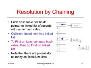
This document discusses hashing techniques for storing data in tables. Hashing allows for fast O(1) insertion, deletion and search times by mapping keys to table indices via hash functions. Collisions occur when different keys hash to the same index, and are resolved using separate chaining (linked lists at each index) or open addressing techniques like linear probing. The load factor determines performance, and tables may need rehashing if they become too full.


![4/18/03 Hashing - Lecture 10 6
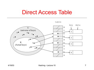
Direct Address Tables
• Direct addressing using an array is very fast
• Assume
› keys are integers in the set U={0,1,…m-1}
› m is small
› no two elements have the same key
• Then just store each element at the array
location array[key]
› search, insert, and delete are trivial](https://image.slidesharecdn.com/lecture10-220909050326-1bc0620b/85/lecture10-ppt-6-320.jpg)
![4/18/03 Hashing - Lecture 10 8
Direct Address
Implementation
Delete(Table T, ElementType x)
T[key[x]] = NULL //key[x] is an
//integer
Insert(Table t, ElementType x)
T[key[x]] = x
Find(Table t, Key k)
return T[k]](https://image.slidesharecdn.com/lecture10-220909050326-1bc0620b/85/lecture10-ppt-8-320.jpg)


![4/18/03 Hashing - Lecture 10 12
“Find” an Element in an Array
• Data records can be stored in arrays.
› A[0] = {“CHEM 110”, Size 89}
› A[3] = {“CSE 142”, Size 251}
› A[17] = {“CSE 373”, Size 85}
• Class size for CSE 373?
› Linear search the array – O(N) worst case
time
› Binary search - O(log N) worst case
Key element](https://image.slidesharecdn.com/lecture10-220909050326-1bc0620b/85/lecture10-ppt-12-320.jpg)
![4/18/03 Hashing - Lecture 10 13
Go Directly to the Element
• What if we could directly index into the
array using the key?
› A[“CSE 373”] = {Size 85}
• Main idea behind hash tables
› Use a key based on some aspect of the
data to index directly into an array
› O(1) time to access records](https://image.slidesharecdn.com/lecture10-220909050326-1bc0620b/85/lecture10-ppt-13-320.jpg)


![4/18/03 Hashing - Lecture 10 27
Characters as Integers
• A character string can be thought of as
a base 256 number. The string c1c2…cn
can be thought of as the number
cn + 256cn-1 + 2562cn-2 + … + 256n-1 c1
• Use Horner’s Rule to Hash! (see Ex. 2.14)
r= 0;
for i = 1 to n do
r := (c[i] + 256*r) mod TableSize](https://image.slidesharecdn.com/lecture10-220909050326-1bc0620b/85/lecture10-ppt-27-320.jpg)