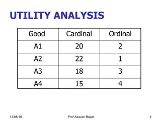
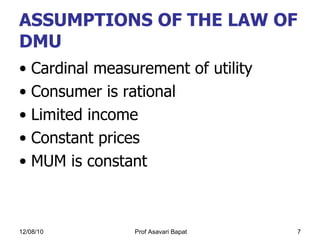
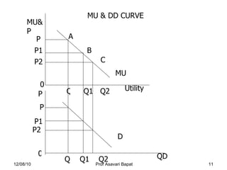
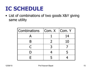
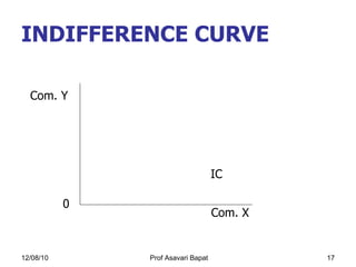
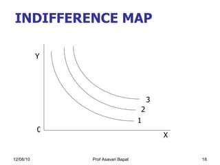
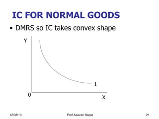
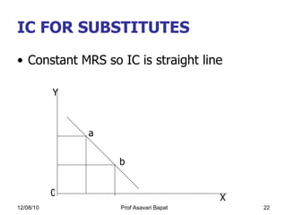
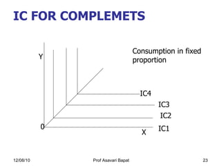
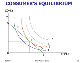
This document discusses key concepts in consumer behavior and consumer choice theory, including: 1) The law of diminishing marginal utility, which states that the marginal utility of additional units of a good decreases as consumption increases. 2) Indifference curve analysis, which uses indifference curves to represent combinations of goods that provide equal utility to a consumer. 3) The concept of consumer equilibrium, which occurs when a consumer allocates their budget in a way that equalizes marginal utility per dollar across all goods purchased. 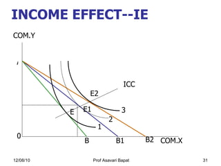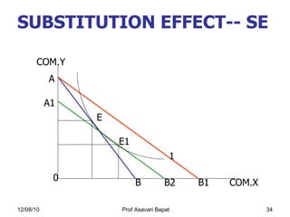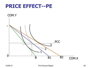4) How changes in income or prices can impact consumer equilibrium through income and substitution effects.

1. CONSUMER BEHAVIOUR Consumer is a king -- buying power, preferences & price signals Preference & choice Objectives To derive maximum utility To pay lowest possible price

2. UTILITY ANALYSIS Utility – capacity of commodity to satisfy human want Cardinal approach -- measurability of utility Ordinal approach – Ranking of utility

3. UTILITY ANALYSIS 4 15 A4 3 18 A3 1 22 A2 2 20 A1 Ordinal Cardinal Good

4. RELATION BETWEEN TOTAL & MARGINAL UTILITY Marginal utility is addition to total utility Total utility increases with every addition at diminishing rate Marginal utility diminishes with every additional unit consumed When total utility is maximum Marginal utility is zero Total utility diminishes when Marginal utility is less than zero

5. THE LAW OF DIMINISHING MARGINAL UTILITY Dr. Marshall states “ the additional benefit which a person derives from a given increase of his stock of a thing diminishes with every increase in the stock that he already has”

6. “ceteris paribus marginal utility from every successive unit consumed goes on declining” Homogeneous units Time period of consumption Consumption up to the point where MU=PRICE

7. ASSUMPTIONS OF THE LAW OF DMU Cardinal measurement of utility Consumer is rational Limited income Constant prices MUM is constant

8. THE LAW OF EQUI-MARGINAL UTILITY The consumer will distribute his given amount of money on different goods in such a way that the marginal utility of last rupee spent on each good is made equal Ratios of MU to P for all goods are equal

9. CONSUMER’S EQUILIBRIUM Maximum satisfaction by allocating income over different goods in such a way that MU of all goods will be in proportion to their respective prices MU of exp. or MU last rupee spent on each good will be made equal MUa/Pa= MUb/Pb=MUc/Pc = ----MUn/Pn

10. DIMINISHING MU & THE LAW OF DEMAND Demand curve slopes downward as MU declines with every additional unit consumed Consumer demands the good till MU = price So lower quantity is demanded at high price & vice versa

11. D MU Q Q1 Q2 Q Q1 Q2 A B C P2 P1 P P P1 P2 QD MU&P 0 0 P Utility MU & DD CURVE

12. LIMITATIONS OF CARDINAL ANALYSIS Measurability of utility questioned Utility is not independent Mum is not constant No distinction between income & substitution effects Unable to explain Giffen paradox Neglects cross effects of related goods Unrealistic

13. INDIFFERENCE CURVE (IC) ANALYSIS Scale of preference the base of IC technique Based of Ordinal measurement of utility Ranking of goods as per satisfaction derived Two goods consumed Independent of Prices & income

14. ASSUMPTIONS OF IC ANALYSIS Rational consumer two goods Income, taste, habits, & prices of goods remain same Comparison and ranking of alternative commodities in order of preference Transitivity Continuity

15. IC SCHEDULE List of combinations of two goods X&Y giving same utility 4 5 E 5 4 D 7 3 C 10 2 B 14 1 A Com. Y Com. X Combinations

16. Techniques of (IC) ANALYSIS Indifference curve A graphical representation of I schedule It is a locus of various combinations of goods giving EQUAL satisfaction Indifference map It is a family/set of ICs

17. INDIFFERENCE CURVE 0 Com. X Com. Y IC

18. INDIFFERENCE MAP 1 2 3 0 X Y

19. MARGINAL RATE Of SUBSTITUTION MRS is the amount of commodity Y given up to obtain additional unit of commodity X 1/1 1:1 4 5 E 2/1 2:1 5 4 D 3/1 3:1 7 3 C 4/1 4:1 10 2 B -- -- 14 1 A ∂ y/∂x MRSxy Com. Y Com. X Combn

20. MARGINAL RATE OF SUBSTITUTION MRS diminishes for normal goods To obtain one more unit of X less & less of Y would be given up So IC takes negative shape

21. IC FOR NORMAL GOODS DMRS so IC takes convex shape 0 X Y 1

22. IC FOR SUBSTITUTES Constant MRS so IC is straight line Y X 0 a b

23. IC FOR COMPLEMETS IC1 IC2 IC3 IC4 0 X Y Consumption in fixed proportion

24. PROPERTIES OF IC All ICs slope downwards from left to right No two ICs intersect IC is convex to origin (reasons) Higher IC represents higher level of satisfaction IC can not touch either axis ICs need not be parallel to each other

25. BUDGET OR PRICE LINE PL shows various quantities of goods can be purchased with given income 0 Com. X Com. y A B X Y M= Pxqx + Pyqy

26. CONSUMER’S EQUILIBRIUM Transformation of scale of preferences into reality by buying certain units of x & y to maximize satisfaction No tendency to rearrange his purchases Constraints faced by Consumer prices of goods Consumer’s income

27. ASSUMPTIONS IC map for X&Y is given Constant prices of X&Y Price ratio remains constant Entire income is spent X & Y are divisible Rational consumer

28. EQUILIBRIUM CONDITIONS The tangency of price line (PL) & IC is necessary condition for equilibrium i.e. slope of PL = slope of IC IC has to be convex at the point of tangency MRSxy=PX/PY = MUx/Px = MUy/Py

29. CONSUMER’S EQUILIBRIUM COM.Y 1 2 3 4 E A B 0 C D Y COM.X

30. INCOME EFFECT--IE Change in real income changes the position of consumer equilibrium Consumer is better/worse off Real income increases or declines Incase of normal goods IE is positive Income consumption curve rises upward

31. INCOME EFFECT--IE COM.Y ICC 1 2 3 A B B1 B2 0 COM.X E E1 E2

32. INCOME EFFECT--IE In case of normal goods IE is Positive If commodity x is inferior IE is negative ICC rises up and bends backward If commodity y is inferior IE is negative ICC rises up and turns downward

33. SUBSTITUTION EFFECT--SE Change in price influences the position of consumer equilibrium Adjustment in money income to maintain real income constant Price effect= Income effect+ substitution effect

34. SUBSTITUTION EFFECT-- SE E E1 1 A COM.X COM.Y 0 B B2 B1 A1

35. PRICE EFFECT--PE Change in price influences the position of consumer equilibrium Consumer is better/worse off Real income increases or declines Incase of normal goods PE is positive PE is negative for inferior/Giffen goods Price effect= income effect+ substitution effect

36. PRICE EFFECT--PE PCC 1 2 3 A B B1 B2 0 COM.Y COM.X

37. DERIVATION OF DEMAND CURVE FROM PRICE CONSUMPTION CURVE

38. SUPERIORITY OF IC ANALYSIS Ordinal utility Consideration of Diminishing MUM Separating price effect into income & substitution effects Explains Giffen's paradox Better way of classifying substitutes & complementary goods Wider application

39. Consumer’s surplus Dr. Marshall defines consumer’s surplus as “excess of the price which a consumer would be willing to pay, rather than go without a thing over that which he actually does pay, is the economic measure of this surplus satisfaction– it may be called consumer’s surplus” Consumer’s surplus= Σ MU - Σ P