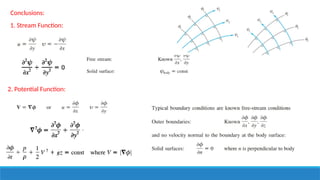
Lecture Four on Stream function and Potential Functions
1.
Potential Flows (forideal flows only)
Learning Objectives:
1. Combination of two or more flow as long as they are govern by linear equations.
2. Set the bases for solving more complex flows
3. Pave the road to the Stream function Concept
4. Laplacian’s Equation can be introduced.
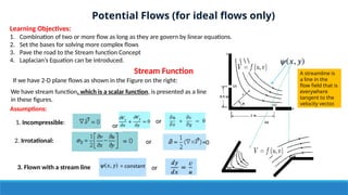
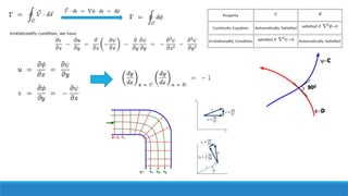
If we have 2-D plane flows as shown in the Figure on the right:
We have stream function, which is a scalar function, is presented as a line
in these figures.
Assumptions:
1. Incompressible:
2. Irrotational:
3. Flown with a stream line
or
or
or
=0
or
A streamline is
a line in the
flow field that is
everywhere
tangent to the
velocity vector.
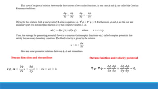
Stream Function
2.
= constant =0
Sub into:
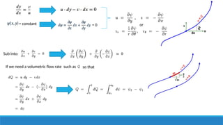
If we need a volumetric flow rate such as so that
or
3.
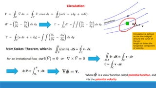
Circulation
Circulation is defined
asthe line integral
around the curve of
the arc
length ds times the
tangential component
of velocity.
From Stokes' Theorem, which is
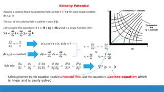
Where is a scalar function called potential function, and
v is the potential velocity
4.
Velocity Potential
or
,
Sub into
Aflow governed by this equation is called a Potential Flow, and the equation is Laplace equation which
is linear and is easily solved
6.
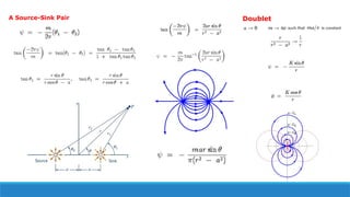
Examples of PotentialFlow solutions
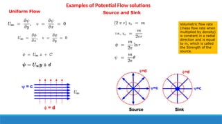
Uniform Flow Source and Sink
Volumetric flow rate
(mass flow rate when
multiplied by density)
is constant in a radial
direction and is equal
to m, which is called
the Strength of the
source.
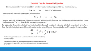
Potential Flow forBernoulli’s Equation
yields
For a potential flow, which is inviscid and irrotational, the Bernoulli equation is extended to include an unsteady term. For a
flow that is inviscid, incompressible, and irrotational, the general form of the unsteady Bernoulli's equation is expressed as: