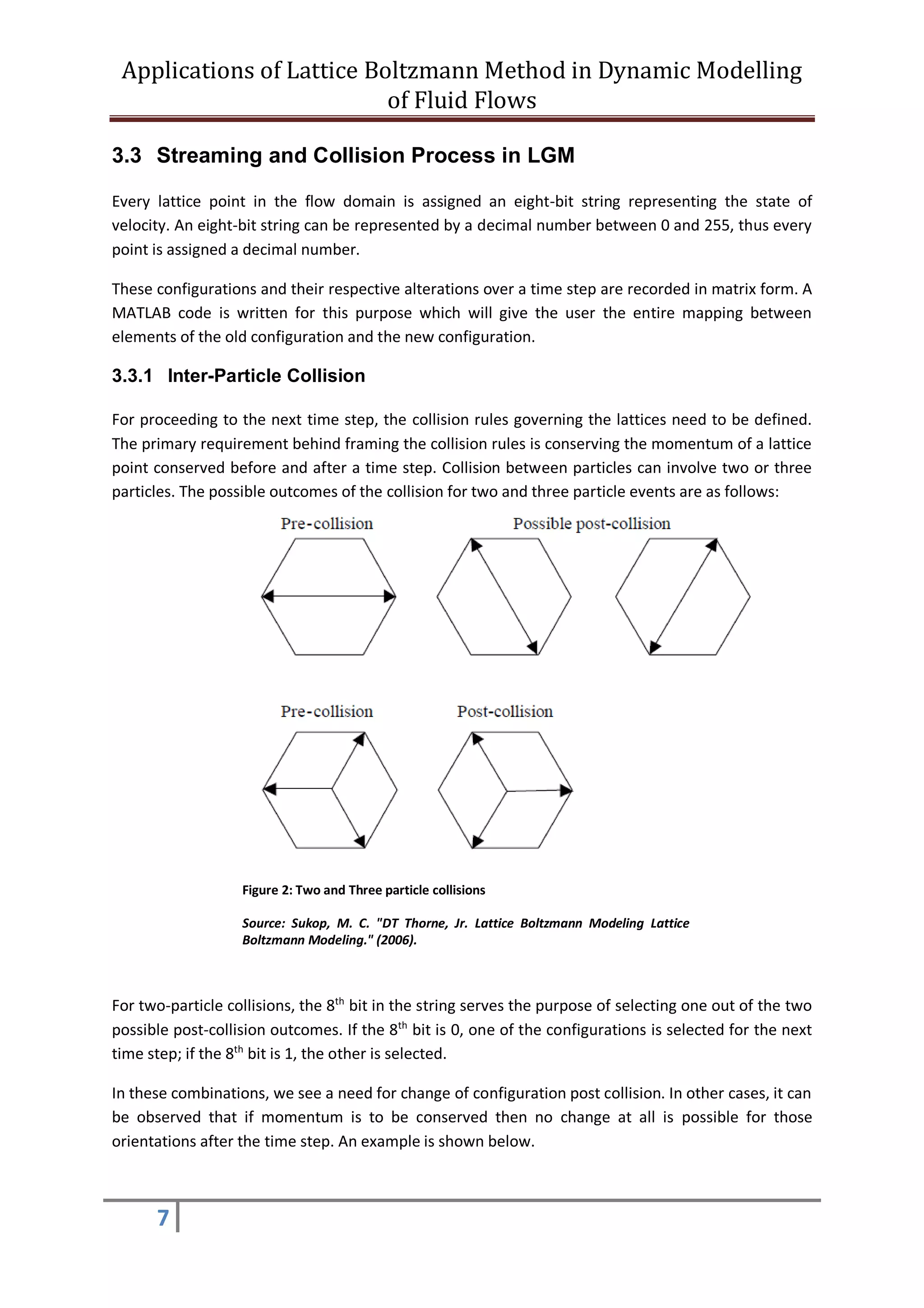
![Applications of Lattice Boltzmann Method in Dynamic Modelling
of Fluid Flows
9
4 The Lattice Boltzmann Method
4.1 Boltzmann distribution function
The LBM simulates the flow patterns of fluids not only in a steady state but also of thermodynamic
systems not in equilibrium. The Boltzmann transport equation describes the statistical behaviour of
such a system in thermodynamic inequilibrium. The equation does not consider the particles
individually, but instead considers all of them together in a probabilistic approach.
A manifestation of this approach can be seen when expressing the particles in terms of the velocities
they carry, and its fractional presence among all the particles present.
When 𝑐 𝑥 𝑐 𝑦 and 𝑐 𝑧 are velocities in the X, Y and Z directions, and 𝑓(𝑐) is the corresponding fraction
of particles having velocity between 𝑐 𝑥 + 𝑑𝑐 𝑥, the total domain may be spanned as
∭ 𝑓( 𝑐 𝑥) 𝑓(𝑐 𝑦)𝑓(𝑐 𝑧) 𝑑𝑐 𝑥 𝑑𝑐 𝑦 𝑑𝑐 𝑧 = 1
The appropriate distribution f can be defined as 𝑓( 𝑐 𝑥) = 𝐴𝑒−𝐵𝑐 𝑥
2
where A and B are constants. Over
the three directions, the products are taken and we obtain 𝑓( 𝑐) = 𝐴3
𝑒−𝐵𝑐 𝑥
2
.
4.2 The Boltzmann Transport Equation
This equation is presented in a modified form when we analyze the effect of external force acting on
a flow domain, with the assumption (for the moment) that no inter-particle collisions are taking
place. The forces are conservative in nature and hence the momentum is conserved.
A system is acted upon by a force F. If 𝑓( 𝑟, 𝑐, 𝑡) be the number of particles having velocity c at
coordinates r at the point of time t when external force F comes to work upon it, assuming there is
no inter-particle collision, the pre- and post-collision states may be related as follows:
𝑓( 𝑟 + 𝑐𝑑𝑡, 𝑐 + 𝐹𝑑𝑡, 𝑡 + 𝑑𝑡) − 𝑓( 𝑟, 𝑐, 𝑡) = 0
However in practical applications there are bound to be collisions between particles, and hence the
collision operator is introduced. The modified form of the equation is
𝑓( 𝑟 + 𝑐𝑑𝑡, 𝑐 + 𝐹𝑑𝑡, 𝑡 + 𝑑𝑡) − 𝑓( 𝑟, 𝑐, 𝑡) = Ω𝑓(𝑑𝑟, 𝑑𝑐, 𝑑𝑡)
This equation can be rewritten in terms of momentum as follows:
𝑓( 𝑥 + 𝑑𝑥, 𝑝 + 𝑑𝑝, 𝑡 + 𝑑𝑡) = 𝑓( 𝑥, 𝑝, 𝑡) + [Γ(+)
− Γ(−)
]𝑑𝑥𝑑𝑝𝑑𝑡
The collision operator Ω can be defined over time dt as the difference of the particles which were
not supposed to arrive at ( 𝑥, 𝑝) but end up there due to collision of particles (Γ(+)
), and the
particles which were supposed to arrive at ( 𝑥, 𝑝) but fail to do so because of collision of particles
(Γ(−)
).](https://image.slidesharecdn.com/applicationsoflatticeboltzmannmethodindynamicmodellingoffluidflows-180420103604/75/Applications-of-Lattice-Boltzmann-Method-in-Dynamic-Modelling-of-Fluid-Flows-9-2048.jpg)
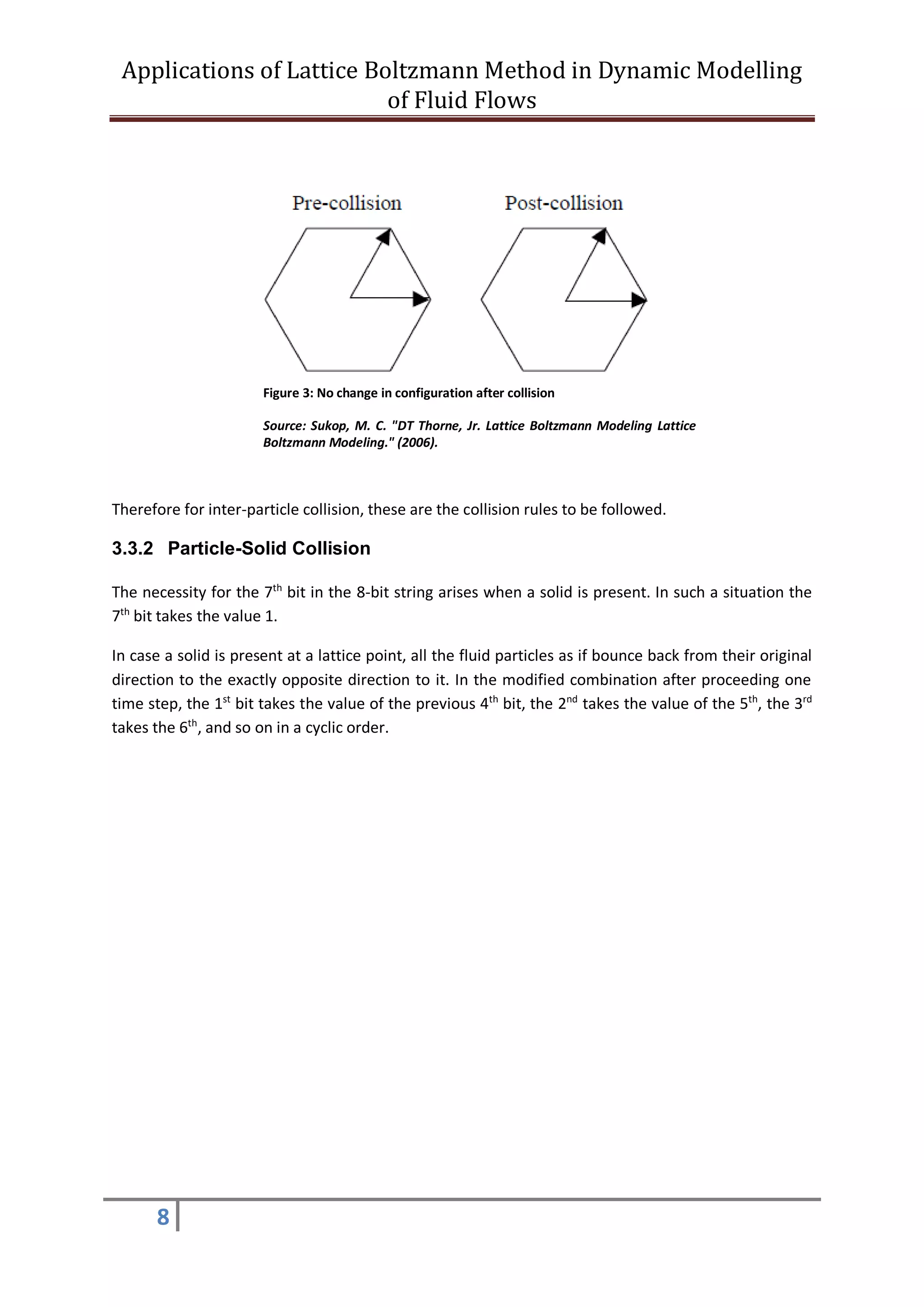
![Applications of Lattice Boltzmann Method in Dynamic Modelling
of Fluid Flows
12
function is called collision operator (Ω). The equation for evolution of the number of the molecules
can be written as
𝑑𝑓
𝑑𝑡
= Ω(𝑓)
The directional derivative being a function of coordinates, speed and time, the first order differential
equation can be written as
𝑑𝑓 =
𝜕𝑓
𝜕𝑟
𝑑𝑟 +
𝜕𝑓
𝜕𝑐
𝑑𝑐 +
𝜕𝑓
𝜕𝑡
𝑑𝑡
∴
𝑑𝑓
𝑑𝑡
=
𝜕𝑓
𝜕𝑟
𝑐 +
𝜕𝑓
𝜕𝑐
𝜕𝑐
𝜕𝑡
+
𝜕𝑓
𝜕𝑡
In absence of any external force,
𝜕𝑐
𝜕𝑡
= 0, and the expression can be further simplified to
𝜕𝑓
𝜕𝑡
+ 𝑐∇f = Ω
4.3.4.1 The BGKW Approximation
The Bhatnagar-Gross-Krook-Welander (BGKW) approximation is used to define the behaviour of the
colliding particles in a simplified way. A collision operator replaced as Ω =
𝑓 𝑒𝑞−𝑓
𝜏
, where 𝜏 is the
relaxation factor.
Collision of the fluid particles is considered as a relaxation towards a local equilibrium (𝑓 𝑒𝑞
). For a
D2Q9 arrangement, the local equilibrium can be derived as follows:
𝑓𝑎
𝑒𝑞
( 𝑥) = 𝑤 𝑎 𝜌( 𝑥)[1 + 3
𝑒 𝑎⃗⃗⃗⃗ 𝑢⃗
𝑐2
+
9
2
( 𝑒 𝑎⃗⃗⃗⃗ 𝑢⃗ )2
𝑐4
−
3
2
𝑢⃗ 𝑢⃗
𝑐2
]
where 𝑤0 =
4
9
, 𝑤1,2,3,4 =
1
9
, 𝑤5,6,7,8 =
1
36
4.3.5 Boundary Conditions
The boundary conditions pose a considerable problem for LBM models. In a lot of cases, no-slip
boundary conditions are present at walls where the fluid velocity is equal to the wall velocity. In this
case, two problems arise. Firstly, due to absence of lattice points beyond the boundaries it is not
possible to obtain certain directional densities through streaming process. Secondly, the lattice
points are defined in terms of directional derivatives and not the velocities itself. So it becomes
difficult to implement things such as the no-slip conditions.
Periodical boundary conditions are sometimes applicable for flows such as flow past solid cylindrical
objects placed periodically causing wake formation. If the flow conditions are identical between two
or more sets of points in the flow range, the first set of simulations can be repeated over the regions
which follow.](https://image.slidesharecdn.com/applicationsoflatticeboltzmannmethodindynamicmodellingoffluidflows-180420103604/75/Applications-of-Lattice-Boltzmann-Method-in-Dynamic-Modelling-of-Fluid-Flows-12-2048.jpg)

This document discusses the Lattice Boltzmann Method (LBM) for modeling fluid flows. LBM is an alternative to directly solving the Navier-Stokes equations using discretization. It is based on the Lattice Gas Automata theory where the fluid domain is divided into discrete lattices inhabited by particles. Governed by rules of streaming and collision, the particle distributions on the lattices are used to model fluid behavior. The document validates LBM by simulating flow through a circular pipe and verifying the results match expected parabolic velocity profiles.