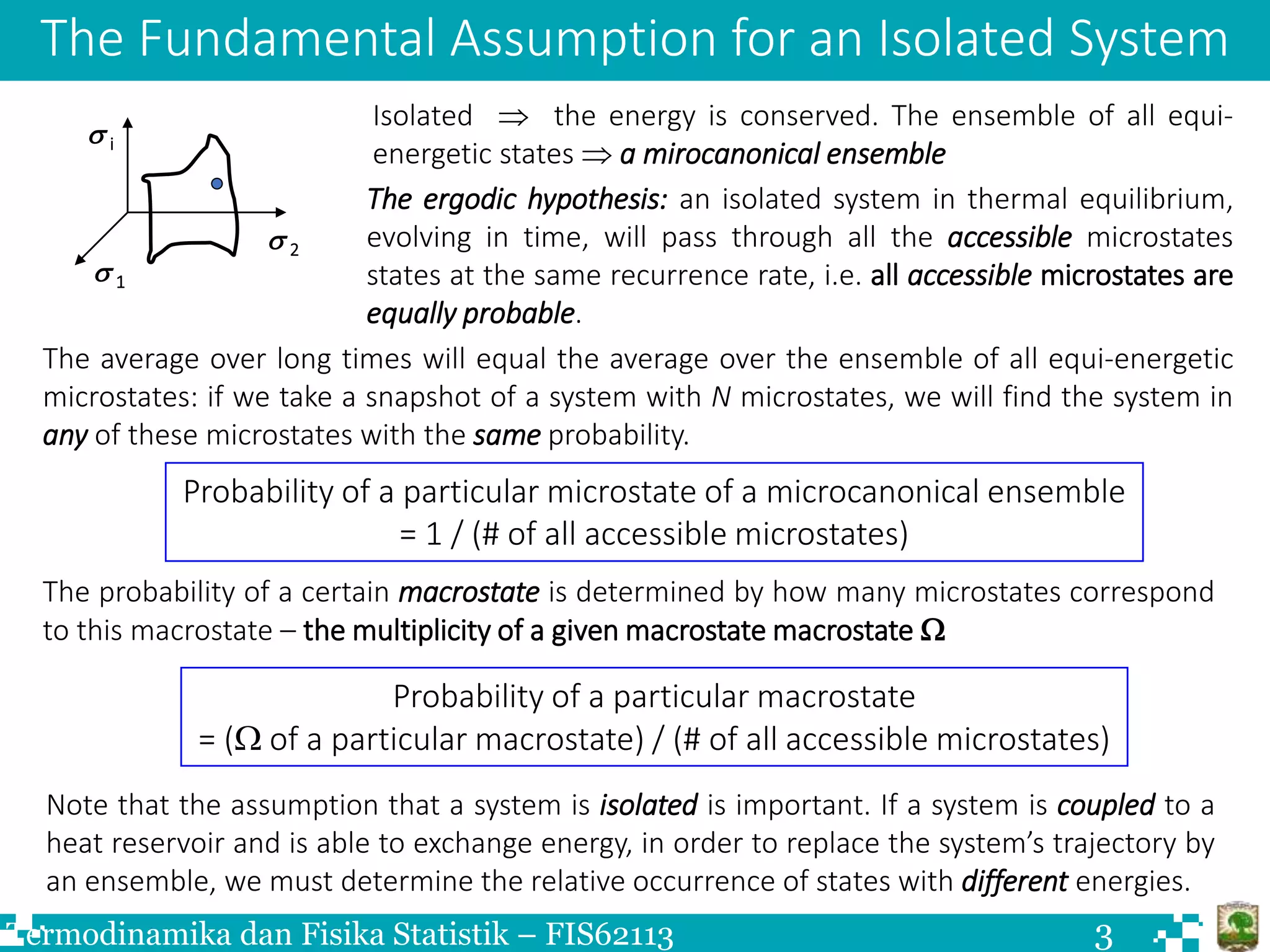
The document discusses Boltzmann statistics and systems in thermal contact with heat reservoirs. It begins by stating the fundamental assumption for isolated systems, which is that all microstates are equally probable. It then discusses how to apply this to systems in contact with heat reservoirs. The key results are:
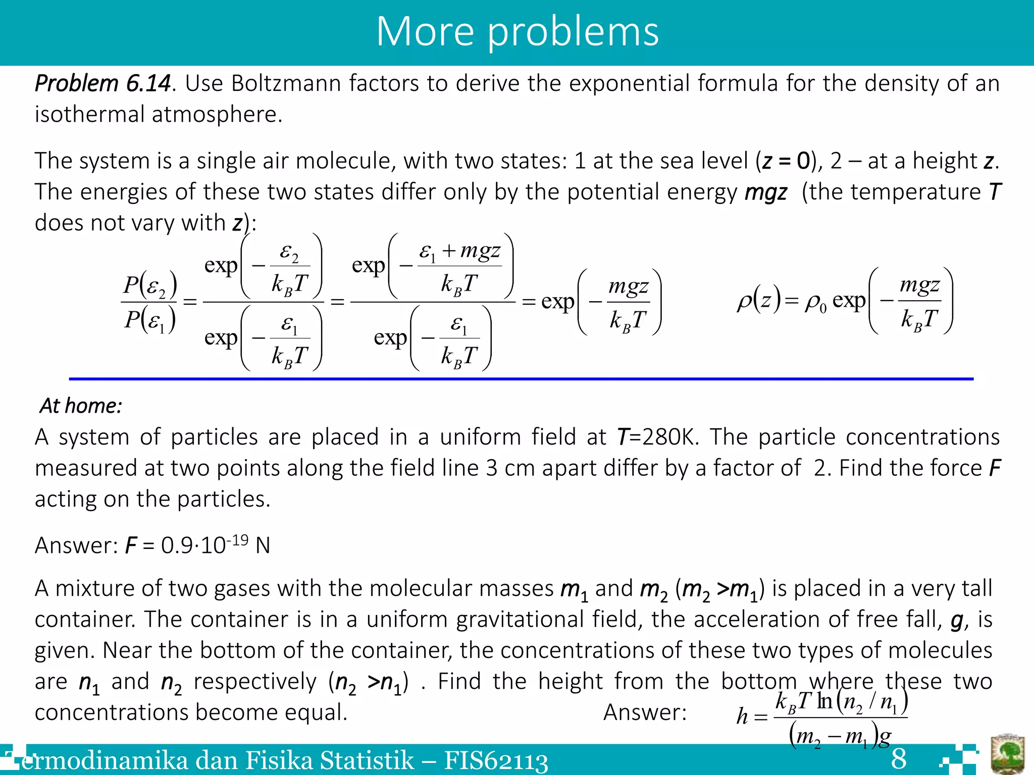
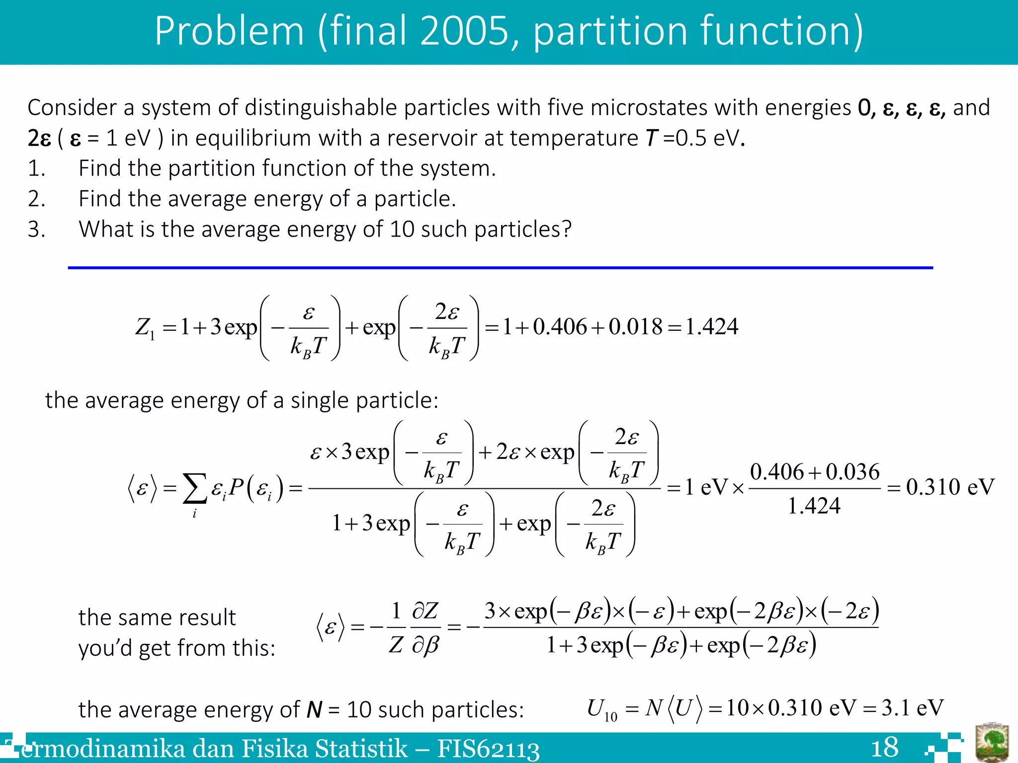
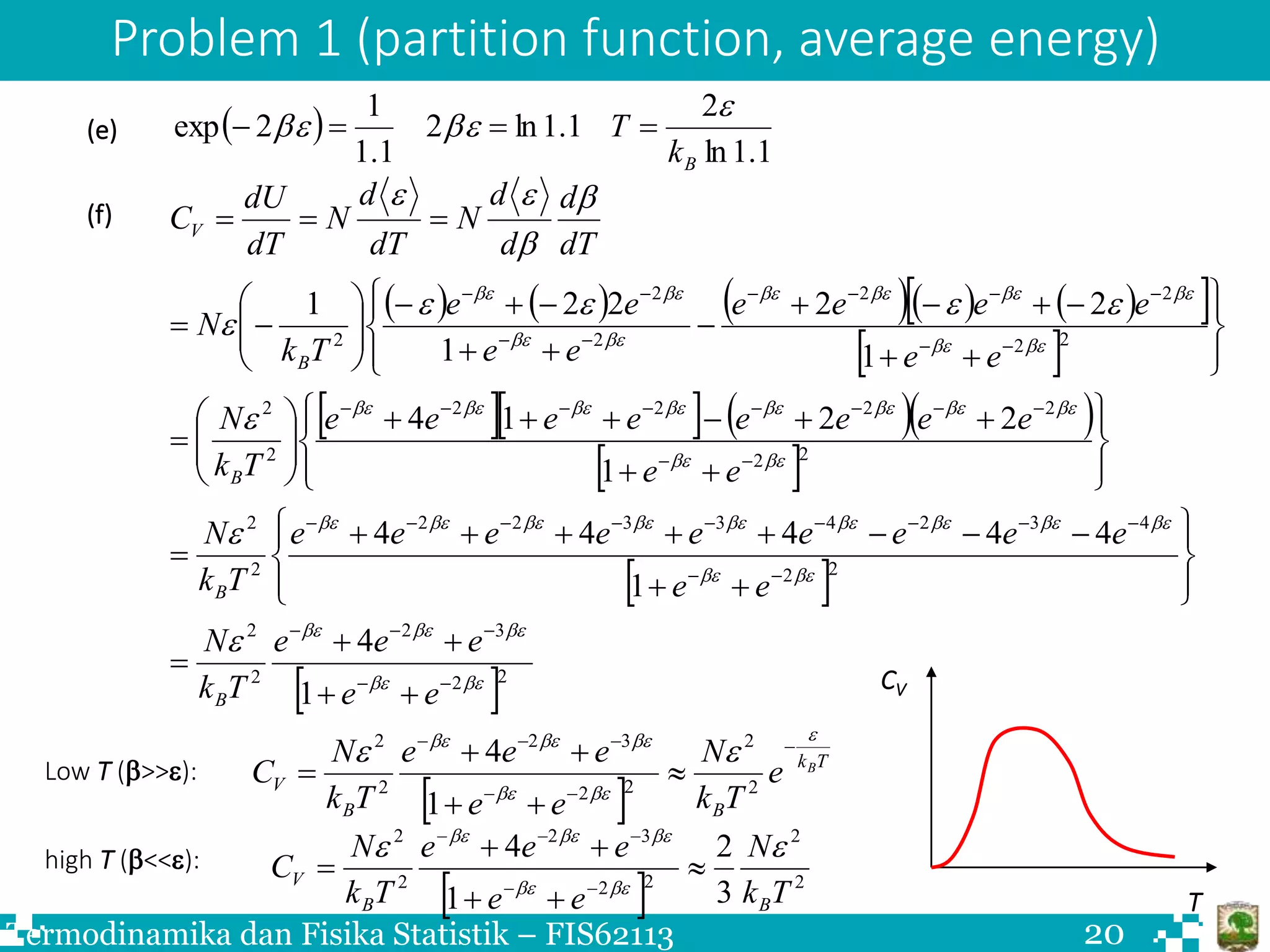
1) For a system in contact with a heat reservoir at temperature T, the probability of the system being in a microstate with energy ε is proportional to the Boltzmann factor e^(-ε/kT).
2) The ratio of probabilities of two microstates with energies ε1 and ε2 is given by the ratio of their Boltzmann factors.
3) Systems visited microstates with