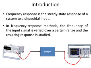
The document discusses frequency response and its relationship to linear systems, describing how sinusoidal inputs yield steady-state sinusoidal outputs that differ in amplitude and phase. It introduces phasors to represent these relationships and discusses frequency domain plots such as Bode and Nyquist plots. The document also details transfer functions and various factors affecting them, including gain, integral and derivative factors, and first-order factors, along with examples of Bode plots.

1. Introduction
• Frequency response is the steady-state response of a
system to a sinusoidal input.
• In frequency-response methods, the frequency of
the input signal is varied over a certain range and the
resulting response is studied.
System

2. The Concept of Frequency Response
• In the steady state, sinusoidal inputs to a linear
system generate sinusoidal responses of the
same frequency.
• Even though these responses are of the same
frequency as the input, they differ in amplitude
and phase angle from the input.
• These differences are functions of frequency.

3. The Concept of Frequency Response
• Sinusoids can be represented as complex numbers
called phasors.
• The magnitude of the complex number is the
amplitude of the sinusoid, and the angle of the
complex number is the phase angle of the sinusoid.
• Thus can be represented as
where the frequency, ω, is implicit.
)
cos( 
 
t
M1 1
1 

M

4. The Concept of Frequency Response
• A system causes both the amplitude and phase angle
of the input to be changed.
• Therefore, the system itself can be represented by a
complex number.
• Thus, the product of the input phasor and the system
function yields the phasor representation of the
output.

5. The Concept of Frequency Response
• Consider the mechanical system.
• If the input force, f(t), is sinusoidal, the steady-state output
response, x(t), of the system is also sinusoidal and at the same
frequency as the input.

6. The Concept of Frequency Response
• Assume that the system is represented by the complex number
• The output is found by multiplying the complex number
representation of the input by the complex number
representation of the system.
)
(
)
( 

 
M
)
(
)
( 

 
M

7. The Concept of Frequency Response
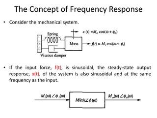
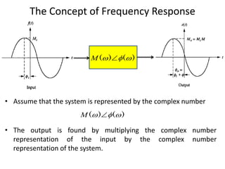
• Thus, the steady-state output sinusoid is
• Mo(ω) is the magnitude response and Φ(ω) is the phase response.
The combination of the magnitude and phase frequency
responses is called the frequency response.
)
(
)
( 

 
M
)]
(
)
(
[
)
(
)
(
)
(
)
( 







 i
i
o
o M
M
M 




8. Frequency Domain Plots
• Bode Plot
• Nyquist Plot
• Nichol’s Chart

9. Bode Plot
• A Bode diagram consists of two graphs:
– One is a plot of the logarithm of the magnitude of
a sinusoidal transfer function.
– The other is a plot of the phase angle.
– Both are plotted against the frequency on a
logarithmic scale.

11. Basic Factors of a Transfer Function
• The basic factors that very frequently occur in
an arbitrary transfer function are
1. Gain K
2. Integral and Derivative Factors (jω)±1
3. First Order Factors (jωT+1)±1
4. Quadratic Factors
)
)(
(
)
(
)
(
2
5
1
1
3
20
2





s
s
s
s
s
s
G

12. Basic Factors of a Transfer Function
1. Gain K
• The log-magnitude curve for a constant gain K is a horizontal
straight line at the magnitude of 20 log(K) decibels.
• The phase angle of the gain K is zero.
• The effect of varying the gain K in the transfer function is that
it raises or lowers the log-magnitude curve of the transfer
function by the corresponding constant amount, but it has no
effect on the phase curve.

13. -15
-5
5
15
Magnitude
(decibels)
Frequency (rad/sec)
0.1 1 10 100
5

K
If db
)
(
(K) 14
5
20
20 
 log
log
Then
103 104 105 106
107
108 109

14. -90o
-300
30o
90o
Phase
(degrees)
Frequency (rad/sec)
0.1 1 10 100
5

K
If 0


 )
5
0
(
tan
)
Re
Im
(
tan
Then 1
-
1
-

103 104 105 106
107
108 109
0o

15. Basic Factors of a Transfer Function
2. Integral and Derivative Factors (jω)±1

j
s
where
s
s
G 
 ,
)
(
)
log(
)
( 
 20

j
G

90
0
1


 
)
(
tan
)
(


j
G
Derivative Factor
Magnitude
Phase
ω 0.1 0.2 0.4 0.5 0.7 0.8 0.9 1
db -20 -14 -8 -6 -3 -2 -1 0
Slope=20db/decade
Slope=6b/octave

16. -30
-10
10
30
Magnitude
(decibels)
Frequency (rad/sec)
0.1 1 10 100
decade
db
20
103 104 105 106
107
108 109
0
-20

17. -180o
-600
60o
180o
Phase
(degrees)
Frequency (rad/sec)
0.1 1 10 100

90

 )
0
(
tan 1
- 

103 104 105 106
107
108 109
0o
900

18. Basic Factors of a Transfer Function
2. Integral and Derivative Factors (jω)±1
• When expressed in decibels, the reciprocal of a number
differs from its value only in sign; that is, for the number N,
)
log(
)
log(
N
N
1
20
20 

)
log(
)
( 

 20
1



j
j
G
Magnitude
• Therefore, for Integral Factor the slope of the magnitude line would
be same but with opposite sign (i.e -6db/octave or -20db/decade).

90
0
1




 
)
(
tan
)
(


j
G
Phase

19. -30
-10
10
30
Magnitude
(decibels)
Frequency (rad/sec)
0.1 1 10 100
decade
db
20

103 104 105 106
107
108 109
0
20

20. -180o
-600
60o
180o
Phase
(degrees)
Frequency (rad/sec)
0.1 1 10 100

90


 )
0
(
tan 1
- 

103 104 105 106
107
108 109
0o
-900

21. Basic Factors of a Transfer Function
3. First Order Factors (jωT+1)
– For Low frequencies ω<<1/T
– For high frequencies ω>>1/T
)
log(
)
( T
j
M 
 
 1
20
)
log(
)
( 2
2
1
20 T
M 
 

0
1
20 
 )
log(
)
(
M
)
log(
)
( T
M 
 20

)
(
)
(
)
( 1
3
1
3 


 s
s
s
G
T
T
1

22. Basic Factors of a Transfer Function
3. First Order Factors (jωT+1)
)
(
tan-1
T


 
)
(

0
0
0 

 )
(
tan
when -1
)
(
, 



45
1
1


 )
(
tan
when 1
-
)
(
, 


T

90




 )
(
tan
when -1
)
(
, 



23. -30
-10
10
30
Magnitude
(decibels)
Frequency (rad/sec)
0.1 1 10 100 103 104 105 106
107
108 109
0
20
)
(
)
(
)
( 1
3
1
3 


 s
s
s
G
ω=3
20 db/decade

24. -90o
-300
30o
90o
Phase
(degrees)
Frequency (rad/sec)
0.1 1 10 100 103 104 105 106
107
108 109
0o
45o

25. Basic Factors of a Transfer Function
3. First Order Factors (jωT+1)-1
– For Low frequencies ω<<1/T
– For high frequencies ω>>1/T
)
log(
)
( T
j
M 
 

 1
20
)
log(
)
( 2
2
1
20 T
M 
 


0
1
20 

 )
log(
)
(
M
)
log(
)
( T
M 
 20


)
(
)
(
3
1


s
s
G

26. Basic Factors of a Transfer Function
3. First Order Factors (jωT+1)-1
)
(
tan-1
T


 

)
(

0
0
0 

 )
(
tan
when -1
)
(
, 



45
1
1




 )
(
tan
when 1
-
)
(
, 


T

90






 )
(
tan
when -1
)
(
, 



27. -30
-10
10
30
Magnitude
(decibels)
Frequency (rad/sec)
0.1 1 10 100 103 104 105 106
107
108 109
0
-20
)
(
)
(
3
1


s
s
G
ω=3
-6 db/octave
-20 db/decade

28. -90o
-300
30o
90o
Phase
(degrees)
Frequency (rad/sec)
0.1 1 10 100 103 104 105 106
107
108 109
0o
-45o

29. Example#1
• Draw the Bode Plot of following Transfer function.
)
(
)
(
10
20


s
s
s
G
Solution:
)
.
(
)
(
1
1
0
2


s
s
s
G
• The transfer function contains
1. Gain Factor (K=2)
2. Derivative Factor (s)
3. 1st Order Factor in denominator (0.1s+1)-1

30. Example#1
)
.
(
)
(
1
1
0
2


s
s
s
G
1. Gain Factor (K=2)
db
K db
6
2
20 
 )
log(
2. Derivative Factor (s)
db/decade
20
20 
 )
log(
db
s
3. 1st Order Factor in denominator (0.1s+1)
0
1
20
1
1
0
1
10 



 )
log(
.
,
db
j

when
db/dec
when 20
1
0
20
1
1
0
1
10 




 )
.
log(
.
, 


db
j

31. -30
-10
10
30
Magnitude
(decibels)
Frequency (rad/sec)
0.1 1 10 100 103 104 105 106
107
108 109
0
-20
)
(
)
(
10
20


s
s
s
G
K=2
20 db/decade
-20 db/decade

32. -30
-10
10
30
Magnitude
(decibels)
Frequency (rad/sec)
0.1 1 10 100 103 104 105 106
107
108 109
0
-20
)
(
)
(
10
20


s
s
s
G
20 db/decade
-20 db/decade+20db/decade

33. Example#1
)
.
(
)
(
1
1
0
2





j
j
j
G
)
.
(
)
( 1
1
0
2 






 

 j
j
j
G
)
.
(
tan
)
(
tan
)
(
tan
)
( 

 1
0
0
2
0 1
1
1 





 j
G
)
.
(
tan
)
( 
 1
0
90 1



 
j
G
ω 0.1 1 5 10 20 40 70 100 1000 ∞
Φ(ω) 89.4 84.2 63.4 45 26.5 14 8 5.7 0.5 0

34. -90o
-300
30o
90o
Phase
(degrees)
Frequency (rad/sec)
0.1 1 10 100 103 104 105 106
107
108 109
0o
-45o
ω 0.1 1 5 10 20 40 70 100 1000 ∞
Φ(ω) 89.4 84.2 63.4 45 26.5 14 8 5.7 0.5 0

35. -20
-10
0
10
20
30
Magnitude
(dB)
10
-1
10
0
10
1
10
2
10
3
0
45
90
Phase
(deg)
Bode Diagram
Frequency (rad/sec)

36. Example#2
)
)(
(
)
(
)
(
100
20
3
20




s
s
s
s
s
G
Solution:
)
.
)(
.
(
)
.
(
.
)
(
1
01
0
1
05
0
1
33
0
03
0




s
s
s
s
s
G