Machine learning process steps

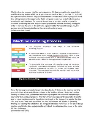
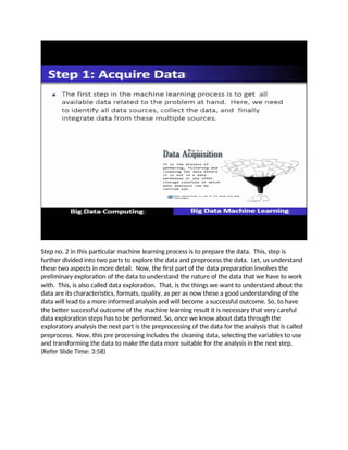
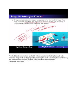
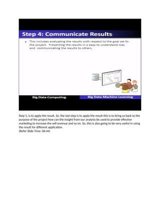
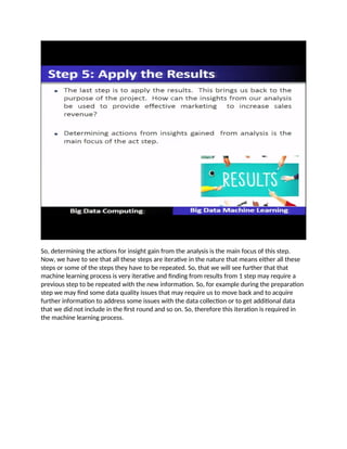
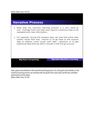
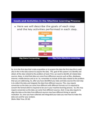
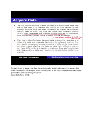
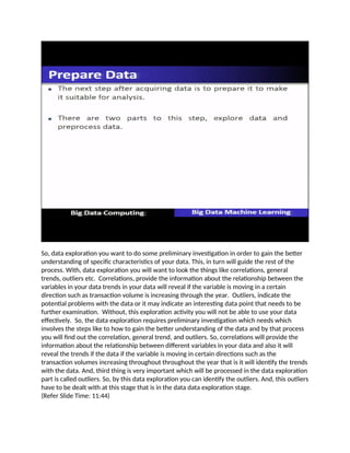
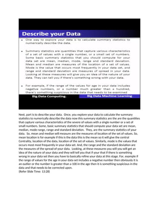
Machine learning process. Machine learning process this diagram explains the steps in the
machine learning process which has Acquire, Prepare, Analyze, Report, and Act. So, it should
be kept in mind that all these steps are needed to be carried out with a clear purpose in mind
that is the problem or the opportunity that is being addressed must be defined with a clear
stated goals and objectives. For example, the purpose of a project may be to study the
customer purchasing behavior. Now, to come up with more effective marketing strategy in
order to increase the sales so this particular aspect must be there at all the steps. So, the
purpose behind the project will drive the machine learning process.
(Refer Slide Time: 01:08)
Now, the first step here is called acquire the data. So, the first step in the machine learning
process is to get all the available data related to the problem at hand. Hence, we need to
identify all data sources, collect the data and finally integrate the data from these multiple
sources for that particular problem. Therefore, the clear purpose or the clear objectives of a
goal in a given problem must be there in the mind while in the step no. 1 to acquire the data.
This, step is also called data acquisition. So, data acquisition is the process of gathering,
filtering and cleaning the data before it is being put in the data warehouse or any other storage
solution on which the data analysis can be carried out. So, data acquisition is one of the major
big data challenges.

Step no. 2 in this particular machine learning process is to prepare the data. This, step is
further divided into two parts to explore the data and preprocess the data. Let, us understand
these two aspects in more detail. Now, the first part of the data preparation involves the
preliminary exploration of the data to understand the nature of the data that we have to work
with. This, is also called data exploration. That, is the things we want to understand about the
data are its characteristics, formats, quality, as per as now these a good understanding of the
data will lead to a more informed analysis and will become a successful outcome. So, to have
the better successful outcome of the machine learning result it is necessary that very careful
data exploration steps has to be performed. So, once we know about data through the
exploratory analysis the next part is the preprocessing of the data for the analysis that is called
preprocess. Now, this pre processing includes the cleaning data, selecting the variables to use
and transforming the data to make the data more suitable for the analysis in the next step.

Third, step is to analyze the data. Now, the prepared data then would be boxed on to the
analysis step. This, involves selecting the analytical technique to use building a model using the
data and assessing the result. Meaning, to say that to analyze the data we require to select one
of these techniques analytical techniques to be used. This, is one of the important decision here
in this step which is to analyze the data. So, techniques involves again all the machine learning
techniques which we have which we have seen that is we have to identify which of these
different categories or classes of machine learning is to be applied to analyze the problem that
is whether it is a classification or it is a regression or it is association or it is clustering. So, all
these techniques we have to identify and within each technique different algorithms are there
that is required to be selection that required to be selected. So, this becomes the selection of
analytical technique to be used in building the model that means we have to fit the model in
the data using these selected techniques. So, this is one of the most important step of a
machine learning.

Fourth, data is to communicate results this include evaluation evaluating the results with
respect to the goal sets for the project. So, presenting the result is in an easy to understand way
and communicating the result to others is also one of the important aspect.

Step 5, is to apply the result. So, the last step is to apply the result this is to bring us back to the
purpose of the project how can the insight from our analysis be used to provide effective
marketing to increase the sell revenue and so on. So, this is also going to be very useful in using
the result for different application.

So, determining the actions for insight gain from the analysis is the main focus of this step.
Now, we have to see that all these steps are iterative in the nature that means either all these
steps or some of the steps they have to be repeated. So, that we will see further that that
machine learning process is very iterative and finding from results from 1 step may require a
previous step to be repeated with the new information. So, for example during the preparation
step we may find some data quality issues that may require us to move back and to acquire
further information to address some issues with the data collection or to get additional data
that we did not include in the first round and so on. So, therefore this iteration is required in
the machine learning process.

Now, goals and activities in the machine learning process. So, the goals and activities in the
machine learning process we will describe the goals from each step and the key activities
performed in these steps.

So, to in the first step that is data acquisition or to acquire the data the first step this is used
also in the in the data science to acquire the data. The, goal of this system is to identify and
obtain all the data related to the problem at hand. First, we need to identify all related data
sources. Keep, in mind that data can come from difference sources such as files, databases,
internet, mobile devices and so on. So, remember to include all the data related to the problem
that you are addressing. So, after you have identified your data and data sources the next step
is to collect the data and integrate the data from different sources. This, may require
conversion as the data can come from different with different formats so it is required to
convert the format which is required to be use in your machine learning process. So, this may
require conversion as the data can come from different sources. And, it may also require to
align the data as the data from different sources may have different timing or special
resolution. So, once you have collected and integrated your data you now have to make this
data core and for your analysis.

Second, step is to prepare the data the next step after acquiring the data is to prepare it to
make it suitable for the analysis. There, are two parts to this step to explore the data and pre-
process that we have already discussed.

So, data exploration you want to do some preliminary investigation in order to gain the better
understanding of specific characteristics of your data. This, in turn will guide the rest of the
process. With, data exploration you will want to look the things like correlations, general
trends, outliers etc. Correlations, provide the information about the relationship between the
variables in your data trends in your data will reveal if the variable is moving in a certain
direction such as transaction volume is increasing through the year. Outliers, indicate the
potential problems with the data or it may indicate an interesting data point that needs to be
further examination. Without, this exploration activity you will not be able to use your data
effectively. So, the data exploration requires preliminary investigation which needs which
involves the steps like to how to gain the better understanding of the data and by that process
you will find out the correlation, general trend, and outliers. So, correlations will provide the
information about the relationship between different variables in your data and also it will
reveal the trends if the data if the variable is moving in certain directions such as the
transaction volumes increasing throughout throughout the year that is it will identify the trends
with the data. And, third thing is very important which will be processed in the data exploration
part is called outliers. So, by this data exploration you can identify the outliers. And, this outliers
have to be dealt with at this stage that is in the data data exploration stage.

Next, part is to describe your data. Once, you explore your data to calculate the summary
statistics to numerically describe the data now this summary statistics are the are the quantities
that capture various characteristics of the severe of values with a single number or a set of
small numbers. Some, basic summary statistics that should compute your data set are mean,
median, mode range, range and standard deviation. They, are the summary statistics of your
data. So, mean and median will measure are the measures of location of the set of values. So,
mean location is for example if this is the data this is the mean so it will give the central
Centrality, location of the data, location of the set of values. Similarly, mode is the values that
occurs most most frequently in your data set. And, the range and the standard deviation are
the measures of the spread of your data. Looking, at these measures you will you will get an
idea of the nature of your data and they will tell you that if your that if there is something
wrong in your data set then you have to basically refine your data at this stage. For, example if
the range of values for the age in your data set includes a negative number then obviously it is
an outlier or the number is greater than a 100 in the age then it is something suspicious in the
data and that needs to be corrected upon.

Now, the next step is called the visualization visualize your data. Visualization techniques, also
provide the quick and effective ways to explore your data. For, example the use of histogram
plots will understand the distribution of data or the skewness or unusual dispersion and outliers
of the data. So, line plot like the one in the lower plot shown over here can be used to look the
trends in the data as the change of the prize on the stock. The, heat map also is one of the
visualization technique of your data give an idea about where the hot spots are. Scatter plots,
effectively show the correlation between the two variables and overall there are many other
type of plots to visualize your data. They, are very useful in helping to understand behavior of
your data.

Now, pre-processing step. So, after you have explored the data the next step is the pre-process
the data to prepare for the analysis. The, goal here is to create the data that will be used for the
analysis. The, main activities of this pre-processing is to clean the data, select the appropriate
variables to use and transform the data as needed.

So, let us see what do you mean by cleaning the data or that data cleaning. A, very important of
data preparation is to clean the data to address many quality issues. Real world data, is nothing
and there are many examples of a quality issues with the data from the real applications
including missing values such as income in the survey duplicate data such as two different
records of the same customers with different addresses. So, inconsistent or invalid data such as
security zip code, noise in the collection of data that distorts the true values outlier such as
numbers larger than 100 on someone’s age is also an essential to detect and address these
issues that can negatively affect the quality of the data.

The, next important part is about the feature selection. Feature selection, first choosing the set
of features to use that is appropriate for the application. Feature selection, can involve
removing redundant or irrelevant features combining features or creating the new features.
So, during the exploration data step you may have discovered that two features are very
correlated. In, that case one of these features can be removed without negatively affecting the
analysis result. For example, the purchase price of a product and the amount of sales tax are
very likely to be correlated similarly the age and the weight of a person are highly correlated.
So, eliminating the sales tax would then be beneficial. So, removing redundant or irrelevant
features will make the subsequent analysis more simpler and more accurate. So, you may also
want to combine the features to create the new ones. For example, adding the applicants
educational level as a feature to a loan approval application would make more sense and there
are also algorithm to automatically determine the most relevant feature that based on various
mathematical properties.

Then, feature transformation. Feature transformation, maps the data from one format to
another format various transformation operations exist for exampling scaling map the data
values to a specific range to prevent any feature from dominating the analysis result. This, is
very important to be handled. So, filtering or aggregation can be used to reduce the noise and
variability in the data. Dimensionality reduction, maps the data to a smaller subset of
dimensions to simply file the subsequent analysis. We, will discuss these techniques how to
prepare the data using future transformation in further slides.

Now, another step is to analyze the data. So, after preparing the data to address address the
quality issues and pre-process it to get in appropriate format the next step would be to use that
particular data for the machine learning process to analyze. The, goal of this the goal of this
step is to build the machine learning model to analyze the data and to evaluate the results that
you get from the model. So, the analysis step starts with this determining the type of problem
you have you began selecting the appropriate machine learning techniques. So, the selection of
machine learning techniques is the important step of analyzing the data. Then, you construct
the model using the data that is also called to fit the machine learning techniques with the data,
fit the model on the data, fit the machine learning. So, that is called the construction of the a
model with the data you have prepared. So, once the model is build you will want to apply this
model to a new data sample to evaluate how well your model behaves. Thus, the data analysis
involves selecting the appropriate techniques for your problem, building the model and
evaluating the results.

Step number four is about the report. The next step in the machine learning process is
reporting the result from your analysis. In, reporting your result it is important to communicate
the insight to make a case for that action to follow. In reporting your result, you will be think
about what to present and how well to present? In deciding what to present, you consider what
main results are what insights you have gained from your analysis and what added the values to
these insight to the application. Keep in mind that, even the negative results are the value will
learning and suggest further avenues or additional analysis. Remember, that all the findings
must be presented so that it informs the decision makers for the further steps. So, in deciding
how to present remember that the visualization is also an important tool in presenting your
results. So, plots and summary statistics discussed earlier, explore in the data exploration can
be used effectively here as well. You, should have the tables with the details from your analysis
as backup if someone wants to take the deeper dive into the results for that purpose. So, in
summary you want to report your findings by presenting your results and the value added with
the graphs using the visualization tools.

Fifth, step is to act. Final step, in the machine learning process is to determine what action
should be taken based on the insights gained. So, what action should be taken based on the
results of your analysis? Should you should you market certain products to specific customer
segment to increase the sales? What inefficiency can be removed from your process? What
incentive should be affective in attracting new customers? So, these are some of the important
actions you can perform based on this analysis of the outcome. So, once the specific action has
been determined the next step is to implement the action. And, things to consider here include
how can the action be added to your application. How will this and users be affected?
Accessing assessing the impact of implementing actions is then necessary to evaluate the result
benefit gained. So, the result of this assessment determines the next step which would suggest
the additional analysis for further opportunities which can which would begin another cycle of
machine learning process.

Generalization and overfitting. So, the it is about the errors in the classification of machine
learning. So, recall that the machine learning model maps the input it receives to an output. So,
for a classification model the model's output is predicted class labels for the input variables and
the true labels is the target labels. So, again in let us see that in the classification model the
model's output is the predicted class labels for the input variables and the true labels are the
target labels meaning to say that if this is the classification model which is shown as the box
whereas the input is the the data which is basically having the input variable input data with
label or it is also called as the label data and which is prepared in this format. So, this particular
classification model will give the the predicted class label which is also there with the with the
data. So, it will give the predicted class. Now, this predicted class this is an output label. Now,
this label can be compared with the with the input label. So, that is what is mentioned over
here. Let, me summarize this. So, the model's output is called the predicted label for the input
variable. So, the model's output is the is called the predicted label class. So, this is the output of
a model. For, the input variable this is the input variable and the true label is the target. So, the
true label is already there. True label is known. So, the predicted label and the true label both
are now compared. The, true label and the predicted output level if both are same so we have
to now compare about these two different labels. So, then if the classifier predicts the correct
classes label for the sample that is a success. And, if the predicted label is different from the
true class label then there is an error. Now, we have to see these two different cases. So, the

error rate then is the percentage of the error made over the entire data sets. That, is the
number of errors divided by the total number of samples in the data set. So, error rate is known
as the misclassification rate or simply the error. So, error is the error rate by the classification
model.
So, let us discuss this machine learning stage that is the classification. Now, this classification
stage is divided into the two parts one is called the training phase and the other is called testing
phase. So, let us see here this is called the training phase and the training phase includes the
the training data which is the labeled data and also requires one machine learning algorithm.
Using, this particular machine learning algorithm will fit on the data and therefore it will
therefore it will build the model based on the the machine learning technique which is applied
on the training data. So, once the model is build this particular model is now available for the
evaluation of the training phase. This, is called training phase. Now, the other phase is called
the testing phase. In testing phase, also we have the the test data and the model which is now
being created. So, the model is the same which is created over the training phase. So, that
particular model will now be given new data and this is called as the test data. It, is the new
data which is not seen by the training phase. So, when a new data is given to the model now
this model will do the predictions based on this test data and it will give the result that is the
output label and it will be compared with the with the target label output label to be compared

with target label. So, this particular way we are going to do the testing. So, based on these
particular analysis of these particular model we are going to see the activities in the testing
phase.
So, therefore let us see more insight into the errors of errors and the classification. The, model
is built using the training data and evaluated on the test data that we have seen in the previous
slides. So, the training and test data are the two different data sets. The, goal in building the
machine learning mold is to have the model perform well on the training as well as on the test
data. So, the model which is which is created will perform well on the training as well as it will
be also perform well in the test data. Now, error rate are simply the error on the training is
refer to as the training error similarly the error on the test data is referred to as the test error.
So, there are two types of errors. So, training error or the test error. Again, to understand we
have to just you have to recall. What, we have done is there were two different phases one was
called the training phase. Training phase, will take the training data and the machine learning
algorithm and it will build a model this particular model will also give an error. Classification
errors which are collected and it is called a training error. Now, this particular model is given
back again is used again in the testing phase and we will have another data that is called test
data. Test data, when it is given to the model now it will perform and it will give an error and
this error is called testing error. So, there are two different type of errors one is called training

error and the other is called testing error. So, the error on the test data is an indication how
well the classifier will perform on the new data.
Now generalization. This, is known as generalization. Generalization, refers to how well your
model performs on a new data that is the data not used to train the model. Now, you want
your model to generalize well to the new data. So, if you model generalizes well then it will
perform well on the data set. That, is similar in the structure to the training data but does not
contain exactly the same sample in the training data. Since, the test error indicates how well
your model generalizes to the new data note that the test error is also called the generalization
error.

Now, there is a concept which is called as overfitting. So, related concept to the Generalization
is called overfitting. So, if your model has a very low training error but has the high
generalization error then it is called the overfitting. Meaning, to say that during the training
phase the error is less but during the testing phase the error is more hence it is called
overfitting. This, means that the model has learned to model has learned to model the noise in
the training data instead of learning the underlying structure of the data hence it is called
overfitting. So, overfitting at these plots illustrates what happens when a model overfits. So, the
training samples are shown as the points and the input to the input to output mapping that the
model has learned is indicated as the curve. So, the plot on the left shows that the model has
learned the underlying data structure as the curve follows the trend of the sample data point as
well. So, here you can see that this curve has learned the the behavior of a data well. Hence, it
is a good fit during the training phase. Now, this there is another example the plot on the right
however shows that the model has learned to model the model has learned to the noise in the
data set for example this is this curve is fitting to the to the noise and it has and this is different
from this particular curve which has fit to the to the underlying structure of the data. So, this is
an example of the overfitting and the left side graph which shows this particular is a good fit.
So, the model which tries to capture every sample point instead of general trend of the samples
together that is the training error and that is generalization error are plotted together during
the model training.

A model that overfits will not generalize well to the new data. So, the model will do well on just
the training data but not perform well on the new data set or rather it will perform poorly. So, a
classifier that performs well on just the training data set will not be only useful. So, it is
essential that the goal of the good generalization performance should be kept in mind before
building the model. So, overfitting and underfitting. So, underfitting occurs when the model is
fitted to the noise in the training data this result is this results in a low training error and high
test error so that is called overfitting. Now, there is another thing which is called underfitting.
Underfitting, on the other hand occurs when the model has not learned the structure of the
data. This, results in high training error and high test error. When, both the errors are very high
that is the training error is also very high and test error is very high then it is called underfitting.
Now, both are undecidable overfitting and underfitting are undecidable. Since, both mean that
the model will not generalize well to the new data. So, overfitting generally occurs when the
model is too complex that is it has too many parameter relative to the number of training
samples. So, to avoid overfitting the model needs to be kept as simple as possible and yet will
solve the input output mapping for a given data set.

Now, let us see what causes overfitting? In, summary overfitting is when your model has
learned the noise in the training data instead of underlying structure of the data. So, you want
to avoid overfitting so your model will generalize well to the new data. Now, let us discuss the
overfitting in the decision trees. Now, decision tree induction that is the decision tree also
referred as the tree induction the tree repeatedly splits the data in a node in order to get
successfully paired subsets of data. So, this is here the the note gets split into three cases.
Here, this note splits into two. So, this particular process of splitting the note and growing the
tree is called tree induction.

Now, let us see the concept of overfitting in this decision trees. Note, that the decision tree
classifier can potentially expand its notes until it can perfectly classify the samples in the
training data. But, if the tree grows the nodes to fit the noise in the training data then it will not
classify the model for a new sample. This, is because the tree has partitioned the input space
according to the noise in the in the data instead of the true structure of the data in other words
it overfits.

So, how to avoid overfitting in the decision tree. So, there are two methods one is called pre-
pruning the other method is called post-pruning. There, are two methods to avoid the
overfitting in decision trees. The, first one is called pre-pruning the other one is called post-
pruning. So, pre-pruning says that to stop growing the tree before it is fully grown why because
in this particular case it is the data is so the tree is fully grown that means it is growing
according to the noise in the data hence it has to be stopped before it is fully grown and so it
will control the number of notes to limit the complexity of the tree. The, second method of
avoiding the overfitting in the decision tree is called post-pruning. Post-pruning, means let the
tree grow to its maximum size and then prune the tree so that it can reduce or it can overcome
from the overfitting.

Now, let us see the pre-pruning step. So, with the pre-pruning the idea is to stop the tree
induction before fully grown tree is build that perfectly fits the training data. To, do this
restrictive stopping conditions for growing tree must be used. For, example noise stops
expanding if the number of samples in the node is less than some minimal threshold. Another
example is to stop expanding the node if the if the improvement in the impurity measures also
below a certain threshold.

Post-pruning, in the post-pruning the tree is grown to a maximum size and then the tree is
prune to removing by removing the nodes using the bottom up approach that is the tree is
trimmed starting with the leaf nodes. The pruning, is done by replacing the subtree with a leaf
node. If, this improves the generalization error or if there is no change to the generalization
error with this replacement.

Now, overfitting in the decision tree in other words if removing the sub trees does not have the
negative effect on generalization error then the nodes in that subtree only add to the
complexity of the tree and not to its overall performance. So, those notes showed be removed
in practice post-pruning tends to give better results. This, is because pruning decisions are
based on the information from the full tree. Pre-pruning, on the other hand may stop the tree
growing process prematurely however post-pruning is more computationally expensive since
the tree has to be expanded on its full size.

Let, us see how the validation set is used for these purposes. So, now we have again looking
back to the same diagram that is the training phase and the testing phase and this particular
process. So, how to avoid the overfitting and recall that the model that over fit does not
generalize well to the new data recall also that overfitting generalizes generally occurs when
the data is too complex. And, how to determine when it should occur.

So, there is a technique which is called using the validation set. A validation set, can be used to
guide the training process to avoid the overfitting and deliver the good generalization
performance. Now, we have discussed having the training set and a test set. So, the training set
is used to build the model and a test set is used to see how the model performs in a new data.
So, the training data is now further divided into two different sets one is called the training data
and the other is called validation data. So, training data is not fully used for the training purpose
but it is divided into the validation data. Let, us see what do you mean by the validation data
which is taken out from the training data. So, this particular validation set is used to guide the
training process to avoid the overfitting and deliver the good generalization how that is all done
we will see.

So, training and validation error. Now, we want to further divide up the training into the
training and the validation set. So, the training set is used to train the model as before and the
validation is used to determine when to stop the training model to avoid the overfitting in order
to get the best result performance. So, let us see that there are two different data sets one is
the training data set which is shown over here that it is giving the errors which is called the
training error. Now, with the validation data set we are also getting the errors and we can now
compare these to graphs. What, we see here at this stage this validation is not consistent with
the training error here it divert. So, this is the position where this particular this is the position
when the the model is not behaving consistently with the validation set and the training set and
there validation and the training error are differs at this point where validation error rate is
more compared to the to the training set error. One, is growing the other is decreasing. So,
therefore this particular at this point the model overfits. So, we have to identify when to at
what stage the growing of the tree has to be used using this particular method. So, now let us
understand this. Then, so the training set is used to train the model as before and the validation
is used to determine when to stop the training model to avoid the overfitting in order to get the
best generalization. So, the so the data is to the idea is to look at the errors of both the training
and the validation set during the model training and the orange line here on the plot is shown
as the training error and the green line is validation. We, see that the model building progress is
along X axis so the number of node increases that is the complexity of the node of the model

increases here as the number of node the complexity. So, we can see that the model
complexity increases at this after beyond this particular stage. The, training error decreases
whereas the validation error increases start increasing. So, when the validation error increases
this indicates that the model is overfitting and resulting into the decreased generalization
performance.
So, when to stop this particular training or tree induction. So, this can be used to determine
when to stop the tree induction where the validation error starts to increase is when you get
the best generalization performance. So, the training so the tree induction should be stopped
here. This, method is using the validation set to determine when to stop the training is referred
to as model selection since you are selecting one from many varying complexities. Note, that
this was illustrated for the decision tree classifier and the same method can be applied to other
machine learning models.

What, are the ways to create and use the validation sets? There, are several ways to create and
use the validation sets to avoid the overfitting. The different models are hold out method,
random subsampling, K-fold cross-validation and leave-one-out cross-validation LOOC.

So, hold out method the first way to use the validation set is a hold out method. This, describes
the scenario that we are that we have discussed where the part of the training is reserved as
the validation set the validation is then is then the hold out set.

This, method we have already seen.

Now, K-fold cross-validation the way to improve the repeated hold out hold-out method is to
use cross-validation. Cross-validation, works as follows. Segment, the data into K number of
disjoint partitions. During, each partition during each iteration one partition is used as the
validation set. Repeat, the process K times each time a different partition for the validation so
each partition is used for validation exactly once this is illustrated in the figure. In the first
iteration, the first partition is used for the validation. In the second iteration, the second
partition is used for the validation and so on.

Now, K-fold cross-validation. The overall validation error is calculated by averaging the
validation for K different iteration. The model with the smallest average validation error is then
selected. The process is just described referred the as K-fold cross-validation. This is very
commonly used approach to model selection in practice. This particular approach gives you the
more structured way to divide available data up between the training and the validation data
set provide a way to overcome the variability in the performance that you can get when using a
using a single partition of the data.

Leave out, leave-one-out cross-validation Leave-one-out cross-validation is a special case of K-
fold cross-validation where K=N, where N is the size of data set. Here for each interaction, the
validation set has exactly one sample. So, the model is trained to use N-1 sample is validated
on the remaining. So, the rest of the process works the same as K-fold cross mode that the
cross-validation is often abbreviated as CV and leave out leave-one-out cross-validation is
referred as LOOCV and pronounced LOOCV.

Uses of validation set. Note, that the validation error that comes out of this process can also be
used to estimate the generalization performance of the model. In other words, the error on the
validation set provides an estimate of the error on the test set.

Uses of data sets with the addition of validation set you really need three distinct data sets
when you build a model. Let us review these data sets. So, we have seen the first type of data
set is called the training data set which is used to train the model that is to adjust the
parameters of the model to learn the input to the output mapping that is called the training
data set. The validation data set is used to determine when the training should stop in order to
avoid overfitting so this is called the validation data set. Third is called the test data set is used
to evaluate the performance of the model on the new data set. So, that means the data set is
divided into three different type of data sets one is called the testing or training data set then it
is the validation data set third is called test data set. Let, us see that the training data set is
used to train the model that is to adjust the parameter of the model to learn the mapping from
input to the output. So, that means training data set will build the model and the validation
data set is used to determine when the training should stop in order to avoid the overfitting. So,
while building the model it will refine this particular model so that it will be improved model
which will not have the overfitting. Finally, the test data set is used to evaluate the performance
of the model. So, this evaluation of this improved model will be done using the test data set.
Now, let us see that how this data set or given data set is divided into three different parts
which are called training data set validation data set and test data set.

So, note that the test data set should never be used in any way to create or tune the model. So,
it should be a new data set which is shown. For example, in a cross-validation process to
determine when to stop the training it should not be used there. So, the test data set must
always remain independent from the model training and remain untouched until the very end
when all the training has been completed. Note, that the sampling the original data set to
created training validation test all the data set must contain the same distribution of the target
class. For example, if the original data set if in the original data 75% samples belong to one class
30% samples to the other class then this same distribution should approximately be present in
each of the training validation and test set otherwise the analysis will be misleading.

So, validation set summary. So, we have discussed the need for three different data sets in the
model building. So, the training set is to train the model the validation set is to determine when
to stop the training process and test to evaluate the performance on the new data. We, have
learned how a validation set can be used to avoid overfitting and in the process to provide an
estimate general performance estimate of generalized performance and the generalization
performance. And, we cover different types to create and use validation set such as K-fold
cross-validation.

Now metrics to evaluate the model performance.

So, here we give the class labels to the data set in supervised learning that is done is the animal
mammal yes or no is the class label.

Now, using this particular target label we now can see the difference between the true target
label this is called target label this is the true label and this is the label which is the predicted
label out of the classification algorithm this is called predicted label. Now, if you compare them
if both the labels are same then the error type is called there is no error and it is called true
positive. When, the true label is no and the predicted is also no then also it is called the true
negative. So, both are not having any errors. Now, when the true label is no but the predicted
label is yes then it is called the false positive. So, this positive is falsely given hence it is called a
false positive. Now, if the true label is yes and the predicted label is no so it is false negative. So,
these different classes we are now going to see this is called the types of classification error. So,
there are four different types of classification error true positive, true negative is there there is
no error and the predicted label is wrongly saying yes then it is called false positive and if the
predicted label is saying wrongly no yeah it is saying wrongly no then it is called false negative.

So, let us see calculate the accuracy rate out of this error types. So, accuracy rate is nothing but
the number of correct predictions divided by total predictions. So, number of correct
predictions here you can see that the true value is yes so it is also predicting yes true is no it is
also saying no and number of correct predictions and here in all other 2 cases it is wrongly
predicted. So, the number of correct predictions is 2 divided by how there are 4 different. So, in
that particular sample we have to find out how many such false positives, false negatives, true
positive and true negatives are there and based on that we can find out the accuracy rate and
error rate is (1- accuracy rate) that is 0.3 here in this case.

So, let us see another thing is called recall and precision says that (
True Positives
True Positiv es+False Positives
). True positives divided by all positives which is predicted by the
the prediction is called precision. And recall is true positives divided by that is true positives and
false negatives ( TruePositives
True Positives+False Positives
) that is all samples with so this is called recall.

So, precision and recall, precision is considered as the major of exactness because it calculates
the percentage of samples predicted as positive which are actually positive in the class. Recall,
is considered as the major of completeness because it calculates the percentage of positive
samples that that the model correctly identifies.

So, besides precision and recall there is something which is called the F-Measure, which
combines both of them. So, F1 measure is nothing but 2∗(
precision∗recall
precision+recall
) where F1 is evenly
weighted that means the precision and recall are given equal weights then it is called F1
measure. And, F2 measure here the weighs recall more in this case and F0.5 measure gives the
weights precision more in this case.

Let, us see the confusion matrix.

So, again we will see that if the animal is the animal mammal so this data set of animal we are
going to label that yes or no.

So, again there are four different classification errors. Based, on these classification errors we
can draw a confusion matrix. So, confusion matrix on the X axis gives the true class label and
whereas the Y is called predicted class label. So, if the true class label is yes and the predicted
class label is also yes then it is called true positive and if the true class label is yes and the
predicted is no then it is called the the false negative. Similarly, if the true class label is no and
the predicted class label is yes then it is called false positive. And, if the true label is no and the
predicted is also no then it is called true negative. So, this particular matrix is called the
confusion matrix.

So, let us see the confusion matrix for this particular example and here in this particular
example we can see that this is the true label and this true times, so so this is the correct this is
correctly predicted and this is also correctly saying. So, yes if it is yes then it is correctly
predicted how many times 1 2 3 so it is 3 times it is appearing and when it is when it is no it is
also correctly predicting negative how many times? 1 2 3 and 4 i.e. 4 times it is correctly
predicting. And, it is when it is no and yes so there it is no and it is there it is no and yes it is one
times it is false positive and the remaining is yes or no 1 and 2 times. So, this we have calculated
the confusion matrix. So, total number of samples is 1 2 3 4 5 6 7 8 9 10 so it is 0.3, 0.2, 0.4, 0.1
so that means number of false positive is 10% and number of true negative so true positive is
30% and so this is the correct outcomes so that means 70% is the accuracy of this particular
case whereas 30% is the inaccuracy.

So, let us see the machine learning tools.

Spark MLlib. Spark MLlib, is the distributed machine learning framework on top of the spark
core. So, this is the spark core and on top of it is the machine learning MLlib library is
positioned. So, machine learning spark MLlib is a distributed machine learning framework. So,
what do you mean by distributed machine learning. We will see that, this machine learning that
means the data is big that the machine learning requires the data so that it will build the model
it will learn the model and it will solve the problem. So, the data is a big data which cannot be
stored on a single system therefore the data is to be stored on a distributed platform and the
machine learning algorithm also to be applied on that distributed way hence it is called the
distributed machine learning. So, spark MLlib is the the distributed machine learning framework
build on top of the spark core. MLlib, is a spark scalable machine learning library consisting of
common machine learning algorithms and utilities including classification, regression,
clustering, collaborative filtering and dimensionality reduction. So, what do you mean by
scalable machine learning library is that the cluster machines can follow the property of scale
out hence the particular algorithm that is machine learning algorithm follows that that
particular property hence it is called as scalable machine learning libraries which is the spark
MLlib.

Now, spark MLlib has library has four different components. So, first component is called
different analysis algorithms for machine learning purpose. So, the all the algorithms which is
machine learning algorithms are available as a part of spark MLlib that is the classification,
regression, clustering and collaborative filtering. Now, besides these algorithm it is also having a
feature which is called a pipeline. So, the so the data scientist working in the big data scenario
they can write their own pipeline and do the and apply the machine learning approach on the
big data using pipeline. We will see in this particular part of the discussion that Spark MLlib
provides much pipeline and how pipeline can be used for big data analytics. Then, another
component of MLlib is called featurization which has two parts very important parts which are
called extraction and transformation. So, we will see what do you mean by these extraction and
transformation in this building up the pipeline. And, it has also the utilities such as linear
algebra and forming different statistics.

Now, let us see the classification algorithm which are available in the spark. First, let us see
what are the steps of our doing the classification in spark. So, these are the steps we will follow
and we will see an example how the classification is performed in the spark. Classification, is to
first step is to load the data into the data frame, second is to drop unused and missing data
item. So, this is the data preparation. Here, is to read the data then we have to create a
categorical variable for the low humidity days so that means we will transform the data to be
required in our format. Then, we have to perform the aggregate features used to make
predictions and that means you have to do a feature engineering or feature selection. And,
then split the data into the training and test data sets. Then, we will create and train the
decision tree and then we will save the predictions to the file
(Refer Slide Time: 65:55).

Let, us see how to read the weather data into the data in spark MLlib or in spark format. So,
here we can see that this is the data file and we have to load using the load data file using SQL
context. So, we are using SQL spark SQL using SQLcontext we will read the data file which is
shown over here using these commands of spark. So, using SQL context we will read this
particular file and the format is given as .CSV and other information. Let, us say header is also
there and infer schema is also available as far as spark SQL. So, we will now read in the form of
a dataframe. So, the weather data will be loaded into dataframes and now if you want to see
what are the different columns after performing this read operation, what are the columns read
then these are the different columns of the data set which is being read into the data frames.
That is, air pressure at 9 am, air pressure air temperature at 9 am, average wind direction at 9
am, average wind speed at 9 am, average wind direction at 9 am, maximum wind speed 9 am,
rain accumulation 9 am, rain duration 9 am. So, these are different columns of your data set
and this column will be used to construct the decision trees later on.

So, the data frame columns are again summarized here in a nice manner.

And, after that then we will prepare the data so that all the unused or the missing data can be
removed. So, use the column name and drop use the column name number and drop from
drop that from the data frame and if when whenever there is a row which is missing and then
we will print the number of rows and columns in the let us see how we can do this to drop this
one data which is having missing data. So, let us see we will find out this one the total count.
So, total count of this one data value is 1064 and we will also see that. So, using df.count() and
the length of that data frame of the columns we will find out the total number of data set and
we will find out how many columns or data is available and if there is a difference so we will
find out those the missing data item and remove it. So, therefore we will calculate the total
number of and we will drop all those we will drop the the missing data item from that particular
column. And, then after that we will see that it comes out to be the data set which does not
have any missed data.

Now, third step is to create the categorical variable for the low humidity days. So, meaning to
say that what we will do here is that wherever the numbers are wherever the values categorical
values are there these variables are to be converted into the number and this conversion can
be performed from categorical data to the numerical data. And here, we can see that these
labels are binarized. So these values are binarized and the values are shown as the categorical
data.

Now, aggregate features will be used to make the predictions and now this particular data set
will be split into once the data is prepared then it will be split into the training and the test
data. So, this will be having 80% and 20%. 80% will be training and 20% will be test data and
then we will randomly split that and using the training data we will now fit we will process it to
build the decision trees. Let, us see how we will do this. So, after doing this here we can see
that we are building the we are setting up the decision tree and in the decision tree pipeline we
have to build and now we will perform the the this one to fit the model. So, model is when it is
fit that training on a training data the model will be the decision tree and once the model is fit
then we will perform the predictions on that particular data.

So, once the the predictions are made we will see the the labels and the prediction values. So,
here you see that all are having same and now we will see prediction accuracy using. So, these
predictions values are now stored on the on the file CSV file.

So, conclusion: in this lecture we have discussed the machine learning techniques. We have also
discussed the tools and algorithms that you can use to create the machine learning models that
learned from the data and to scale those models up to the big data problem. Thank you.

Machine learning process steps

Machine learning process steps

Recommended

Recommended

More Related Content

What's hot

What's hot (20)

Similar to Machine learning process steps

Similar to Machine learning process steps (20)

More from vishal choudhary

More from vishal choudhary (20)

Recently uploaded

Recently uploaded (20)

Machine learning process steps