Download to read offline


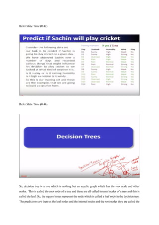
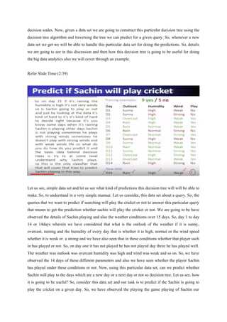
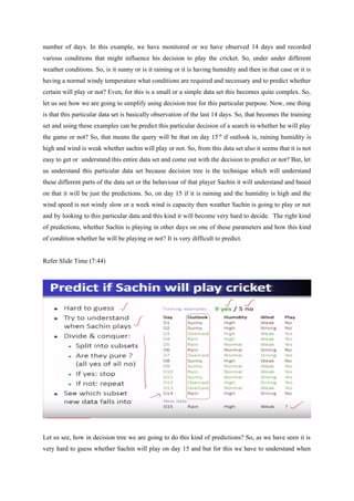
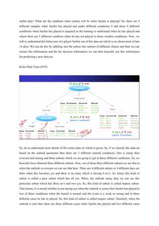
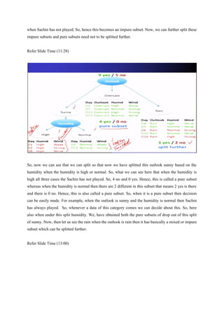
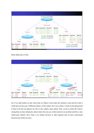
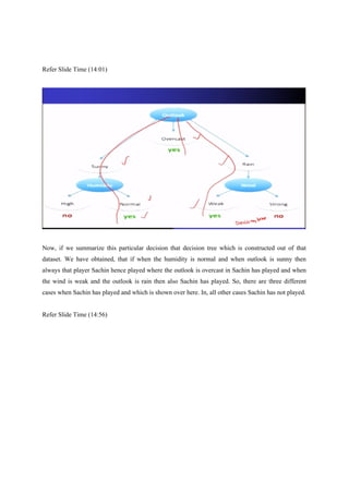
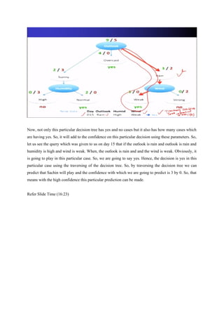
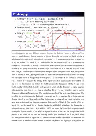
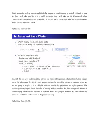
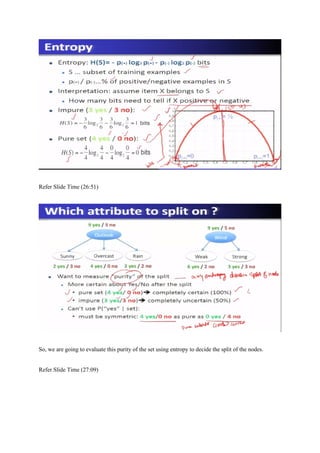
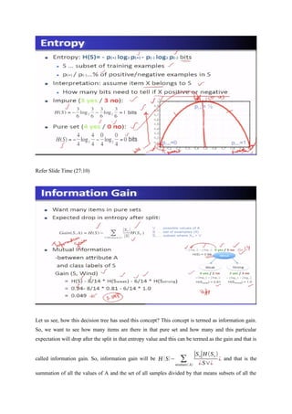
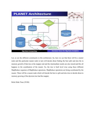


This document discusses using decision trees for big data analytics and provides an example using a dataset to predict whether a cricket player named Sachin will play or not based on weather conditions. The dataset contains observations over 14 days with weather outlook, humidity, wind speed and whether Sachin played. The decision tree splits the data into subsets based on weather parameters to determine conditions when Sachin played versus did not play. This results in "pure" and "impure" subsets that can be split further. The tree shows that when outlook is sunny and humidity is normal, or outlook is overcast, or outlook is rain and wind is weak, Sachin played. All other conditions result in Sachin not playing. The tree can then be used to