Download to read offline


![Theory
Then the process of knowing the value of f(x ) for some unknown
value of x not explicitly given in the interval [a, b] is called
interpolation. The value thus, determined is known as Interpolated
value.
If, y = f(x) takes the values y0, y1, … , yn corresponding to x = x0,
x1 , … , xn then
.
Interpolation polynomial in the Lagrange form is a linear
combination
of Lagrange basis polynomials for 0<j<k:](https://image.slidesharecdn.com/20463986-230523150002-c868c100/85/Lagrange-Interpolation-3-320.jpg)


![Output
X Y
1980 440
1985 510
1990 525
1995 571
2005 500
2005 600
>>
x=[1980,1985,1990,1995,2000,2005];
>> y=[440,510,525,571,500,600];
>> xx=1998;
>> k=3;
>> Lagrange(x,y,xx,k)
Input data of crop production
in tonne for years 1980 to
2005 as given in the table](https://image.slidesharecdn.com/20463986-230523150002-c868c100/85/Lagrange-Interpolation-6-320.jpg)

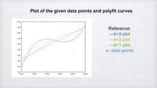


The document describes implementing Lagrange interpolation and least squares polynomial fitting in MATLAB. It includes: 1) An M-file to calculate interpolated values using Lagrange basis polynomials for given x and y data and test point xx. 2) Using polyfit to find the coefficients of a polynomial of degree k that best fits the given x and y data in a least squares sense. 3) Plotting the original data points and polynomial curves for different values of k to visualize the fitting.