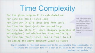
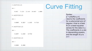
1. The document describes implementing Newton Gregory backward interpolation and least squares polynomial curve fitting in MATLAB. 2. It presents the theory of interpolation, the Newton Gregory backward interpolation formula, and the program steps to calculate backward interpolation for a given data set and plot the results. 3. The time complexity of the backward interpolation program is O(n^2) due to nested loops and other operations that are proportional to the number of data points.

1. PRACTICAL
Name- Saloni Singhal
M.Sc. (Statistics) II-Sem.
Roll No: 2046398
Course- MATH-409 L
Numerical Analysis Lab
Submitted To: Dr. S.C. Pandey

2. OBJECTIVE
1. Create an M-file to implement
Newton Gregory Backward Interpolation.
1. Curve Fitting- Least Square nth order
polynomial to data.

3. Theory
Then the process of knowing the value of f(x ) for some unknown
value of x not explicitly given in the interval [a, b] is called
interpolation. The value thus, determined is known as Interpolated
value.
This Newton Gregory Forward Interpolation formula is useful
when the value of f(x) is required near the end of the table. h is
called the interval of difference and u = ( x – an ) / h, Here an is
last term .
Error term of the formula:

4. Program
clear;
%input number of data points
n= input('enter number of data points=');
%input abscissa and ordinate value
for a=1:n
X(a)= input('enter X'+string(a));
end
for b=1:n
Y(b)= input('enter Y'+string(b));
end %enter the value to be interpolated using
forward interpolation
x=input('enter value of x to be interpolated');
%step size h and d gives the forward difference
table
h=X(2)-X(1);
for i=1:n-1
d(i,1)=Y(i+1)-Y(i);
end
for j=2:n-1
for i=1:n-j
d(i,j)=d(i,j-1)-d(i-1,j-1);
end
end

5. Program Contd.
P1=linspace(min(X),max(X),51);
P2=zeros(51,1);
for i=1:51
P2(i)=nb(P1(i),X,Y,n,d);
end
%plot for the given points
plot(X,Y)
hold on
%plot for the interpoated curve
plot(P1,P2)
hold off
d
nb(x,X,Y,n,d)
% function to calculate the forward inoterpolation
function y=nb(u,X,Y,n,d)
h=X(2)-X(1);
p=(u-X(n))/h;
prod=1;
y=Y(1);
for t=1:n-1
prod=prod*(p+t-1)/t;
y=y+prod*d(n-1,t);
end
end

6. Time Complexity
6
For the given program it is calculated as:
For line 14= 2(n-1) since loop
For line 16= (n-1)+1 since loop from 1:n-1
For line 18= 2(n-1)(n-2) for nested loop
For line 24= 51(6n-3) since linspace generates 51
values(given) and min/max has time complexity n
For line 36= (6n-3) since loop is from i to n-1
on adding the above dominant value is =O(n2)
Big O notation is the most common metric for calculating time complexity. It
describes the execution time of a task in relation to the number of steps
required to complete it.
We calculate the
no of operations in
respective loops
and function.
Big ‘O’ notation
takes its dominant
value

7. Output
>intbackward
enter number of data points=
5
enter X1
0
enter X2
1
enter X3
2
enter X4
3
enter X5
4
enter Y1
1
enter Y2
-1
enter Y3
1
enter Y4
-1
enter Y5
1
enter value of x to be interpolated
3.5

8. Plot of the given data points and interpolated curve
Reference:
— Data Points
plot
—Interpolated
curve

9. Curve Fitting
Syntax:
p = polyfit(x,y,n)
returns the coefficients
for a polynomial p(x) of
degree n that is a best
fit (in a least-squares
sense) for the data in y.
The coefficients in p are
in descending powers,
and the length of p is
n+1

10. Conclusion
• The interpolated value of the point is as shown
in figure.
• Polyfit of degrees less than the number of data
points fits the given oscillatory curve X Y
0 1
1 -1
2 1
3 -1
4 1

11. Caveats
• Newton’s backward difference formula is best
suited when sx lies in the end of data table. Then, it can be
seen that for those values of sx , which lie almost in the
middle of the data table neither Forward or Backward
retains sufficient number of terms in the formula and thus
the interpolated value will not be sufficiently accurate.
• To overcome this problem we derive two more formulae
named as Stirling's formula and Bessel’s formula