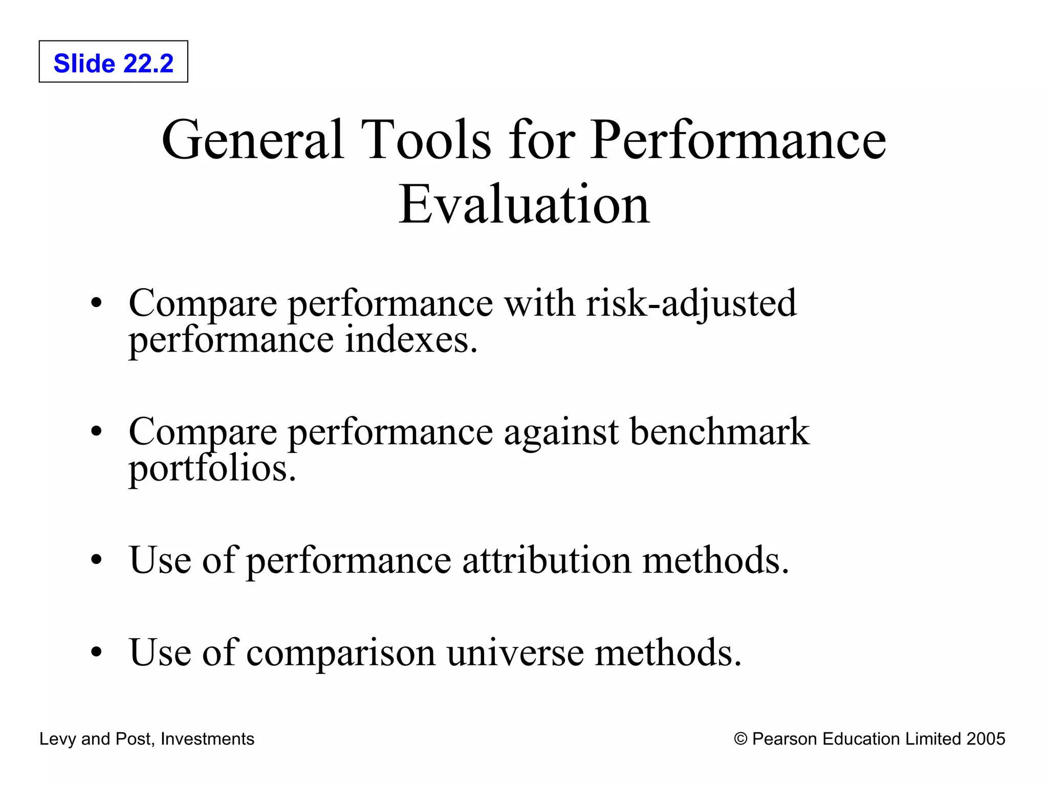
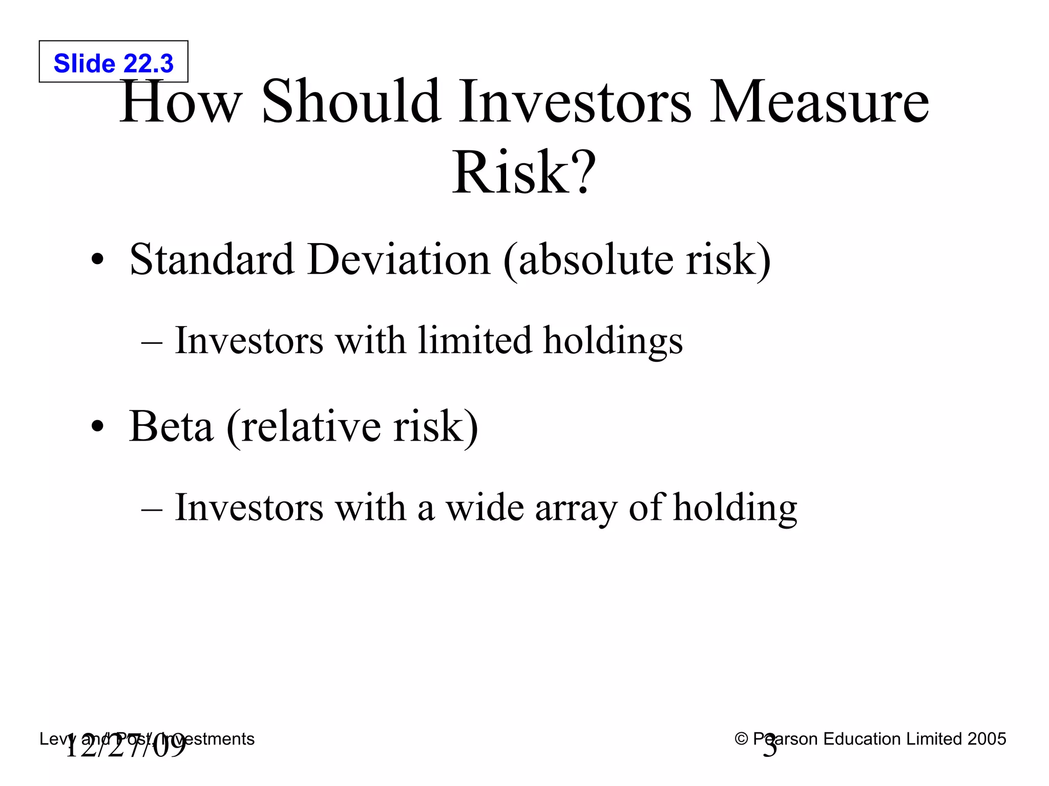
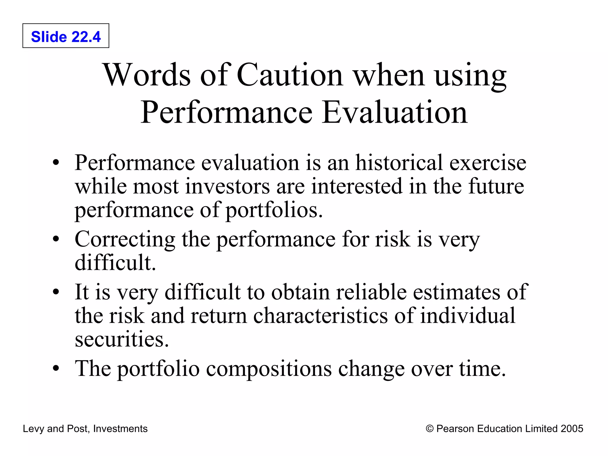
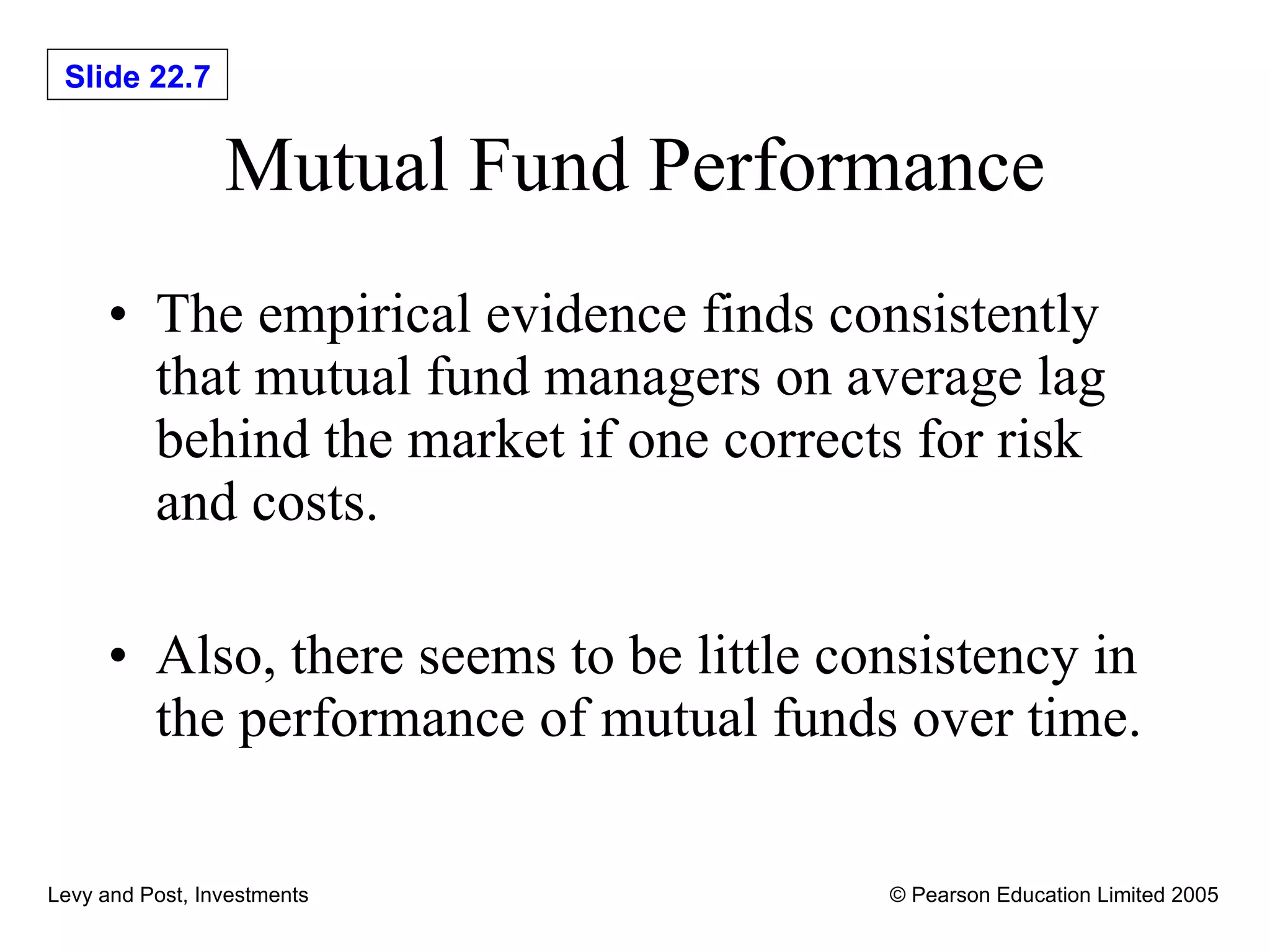
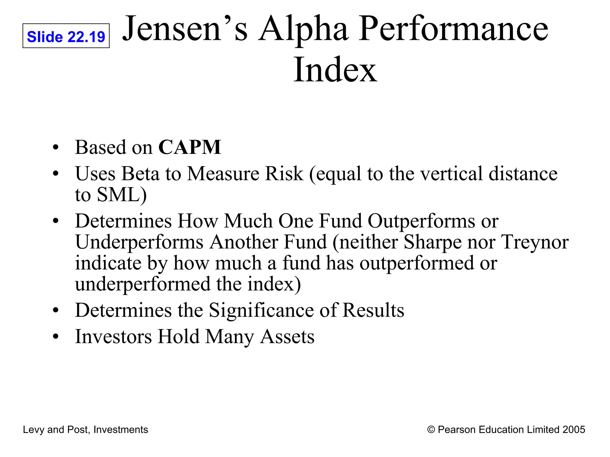
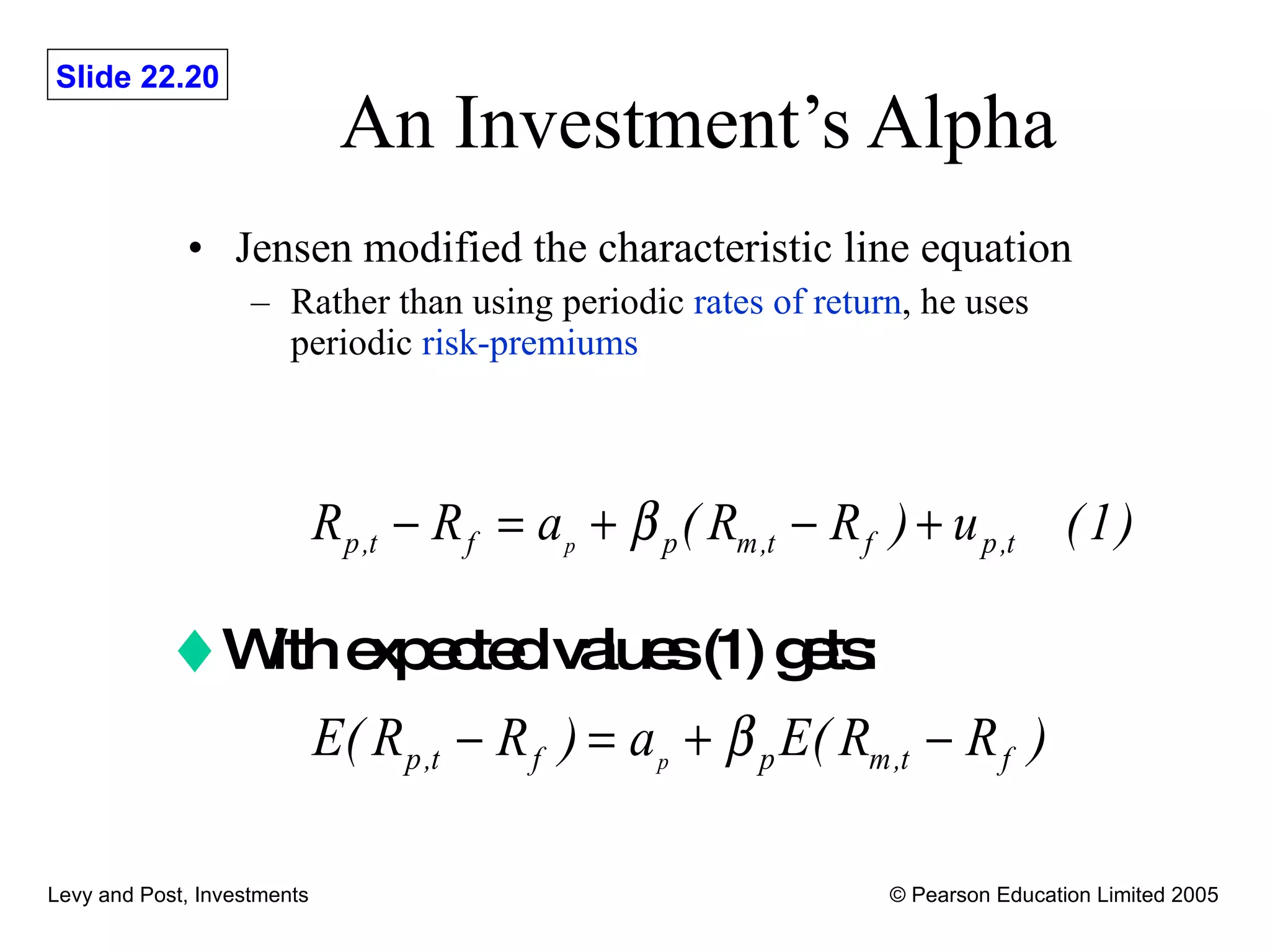
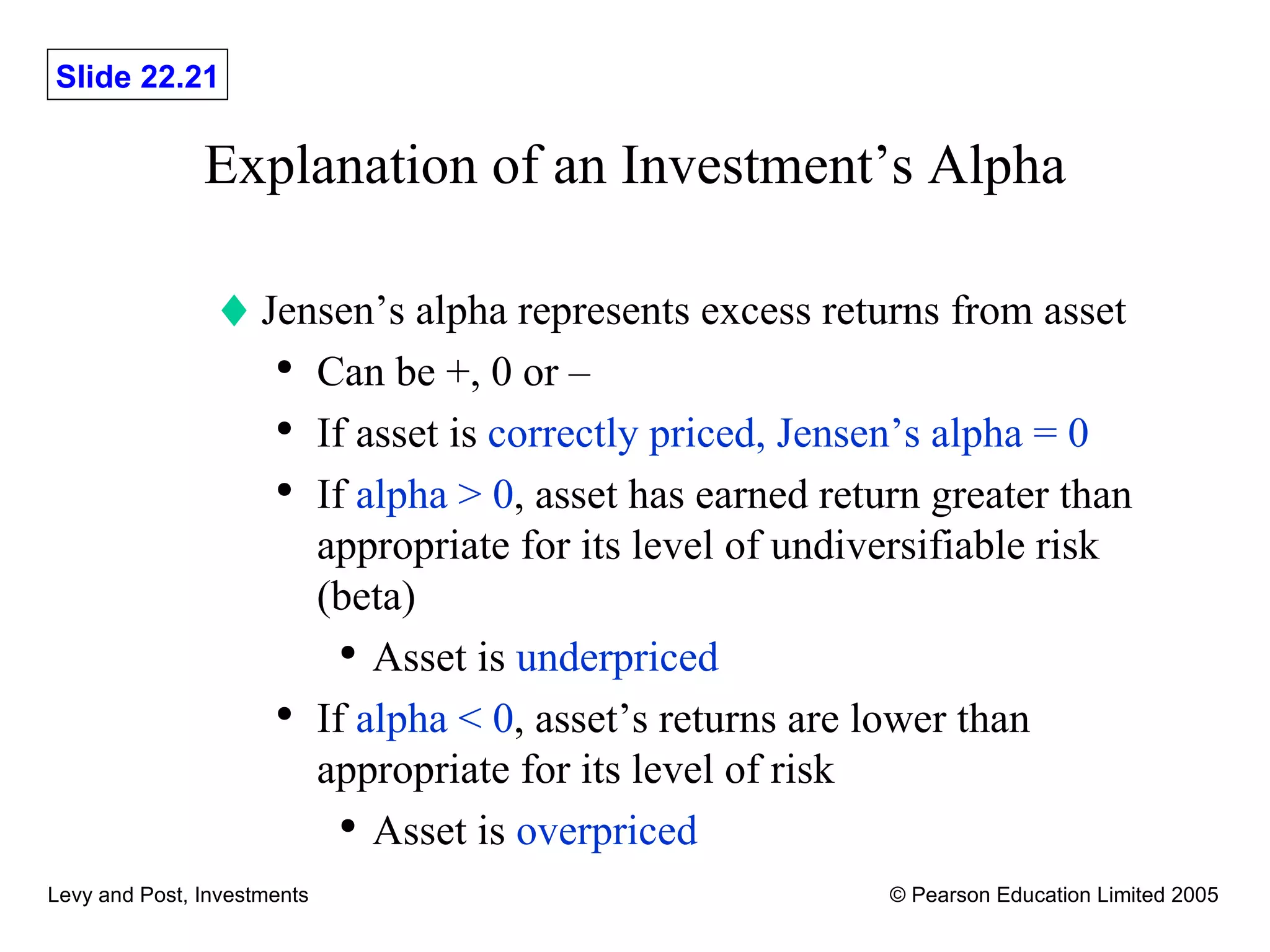
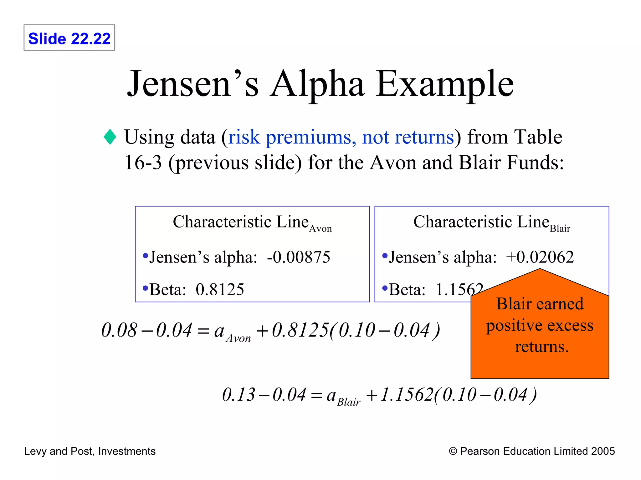
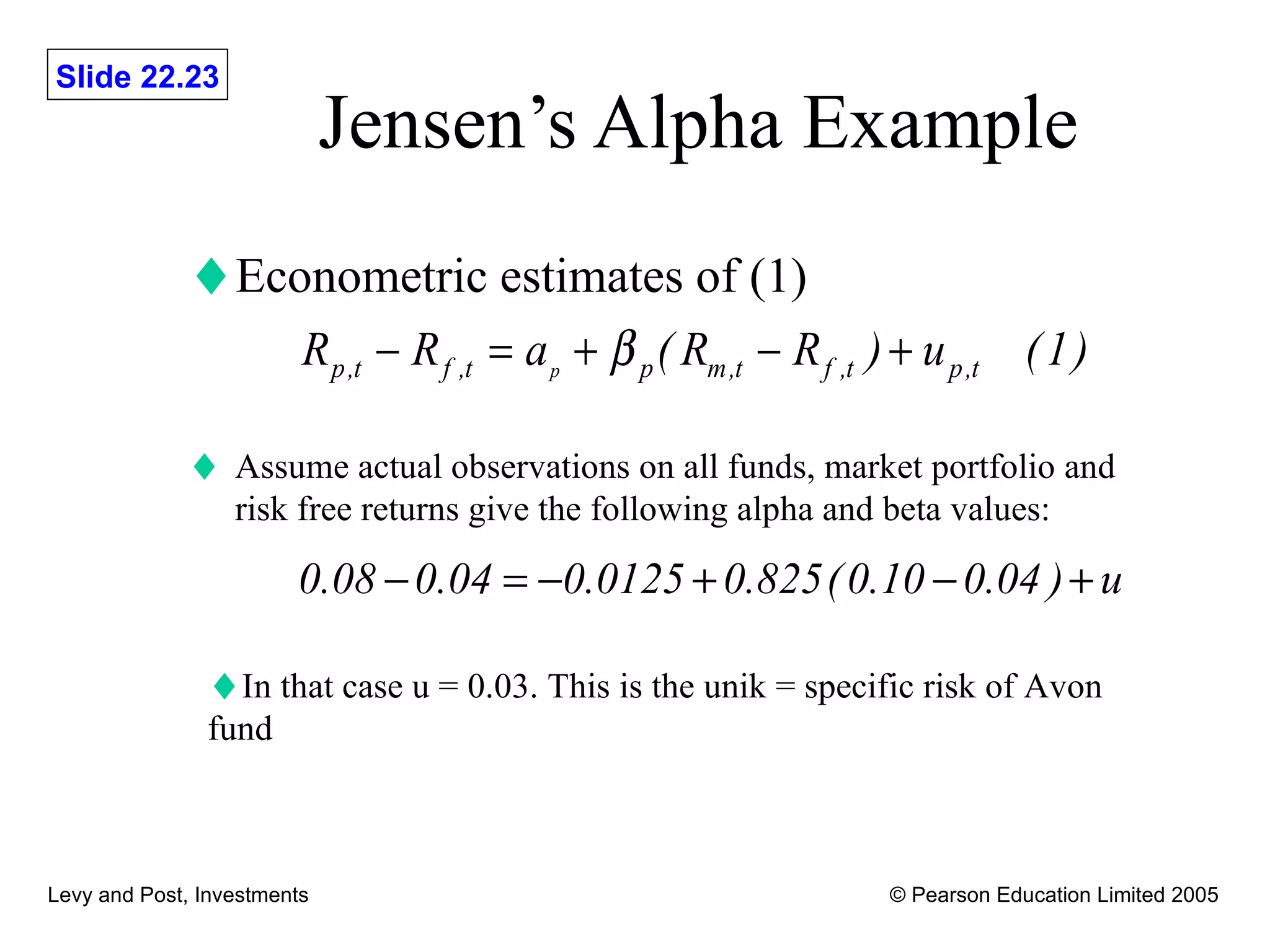
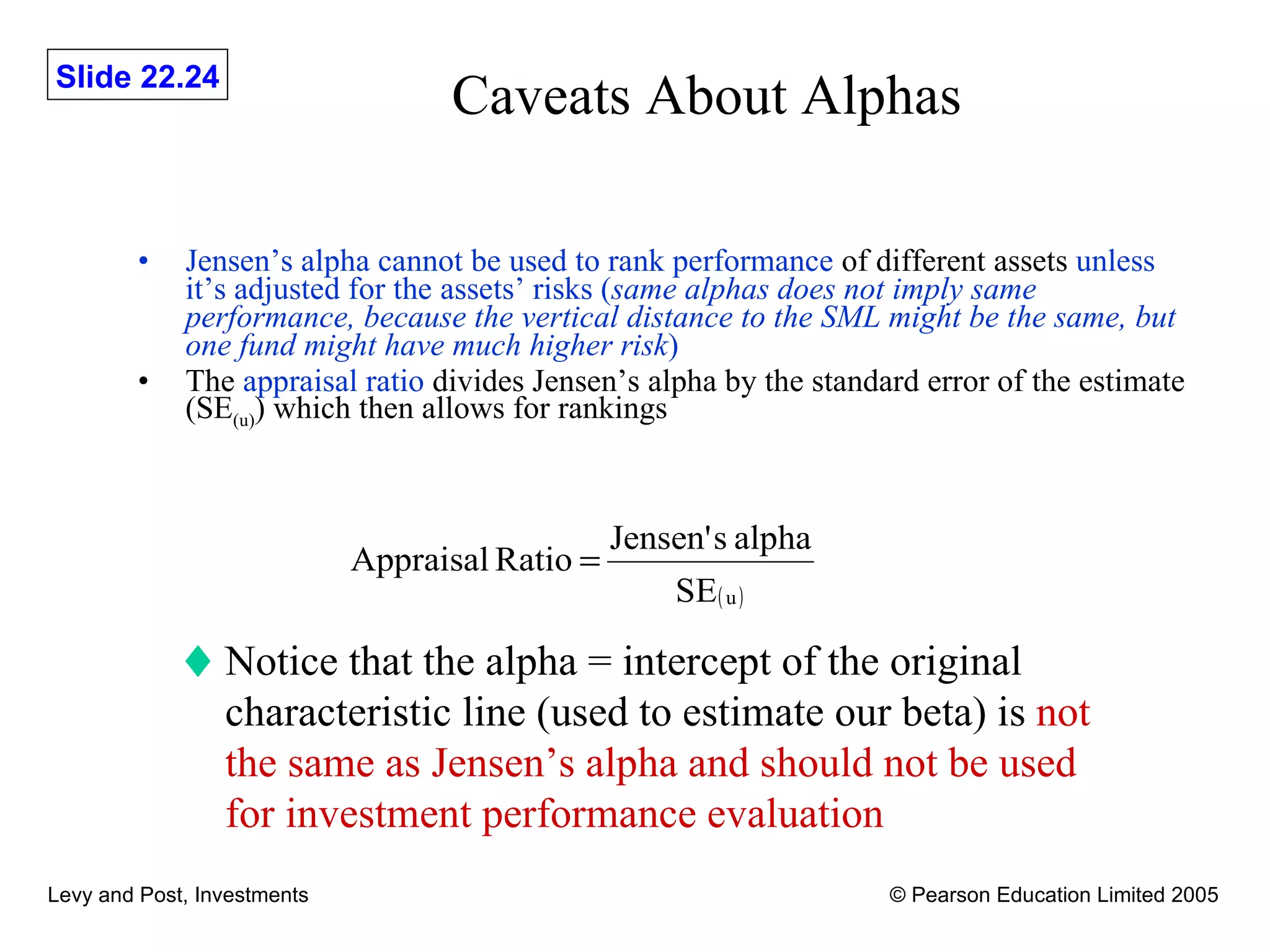
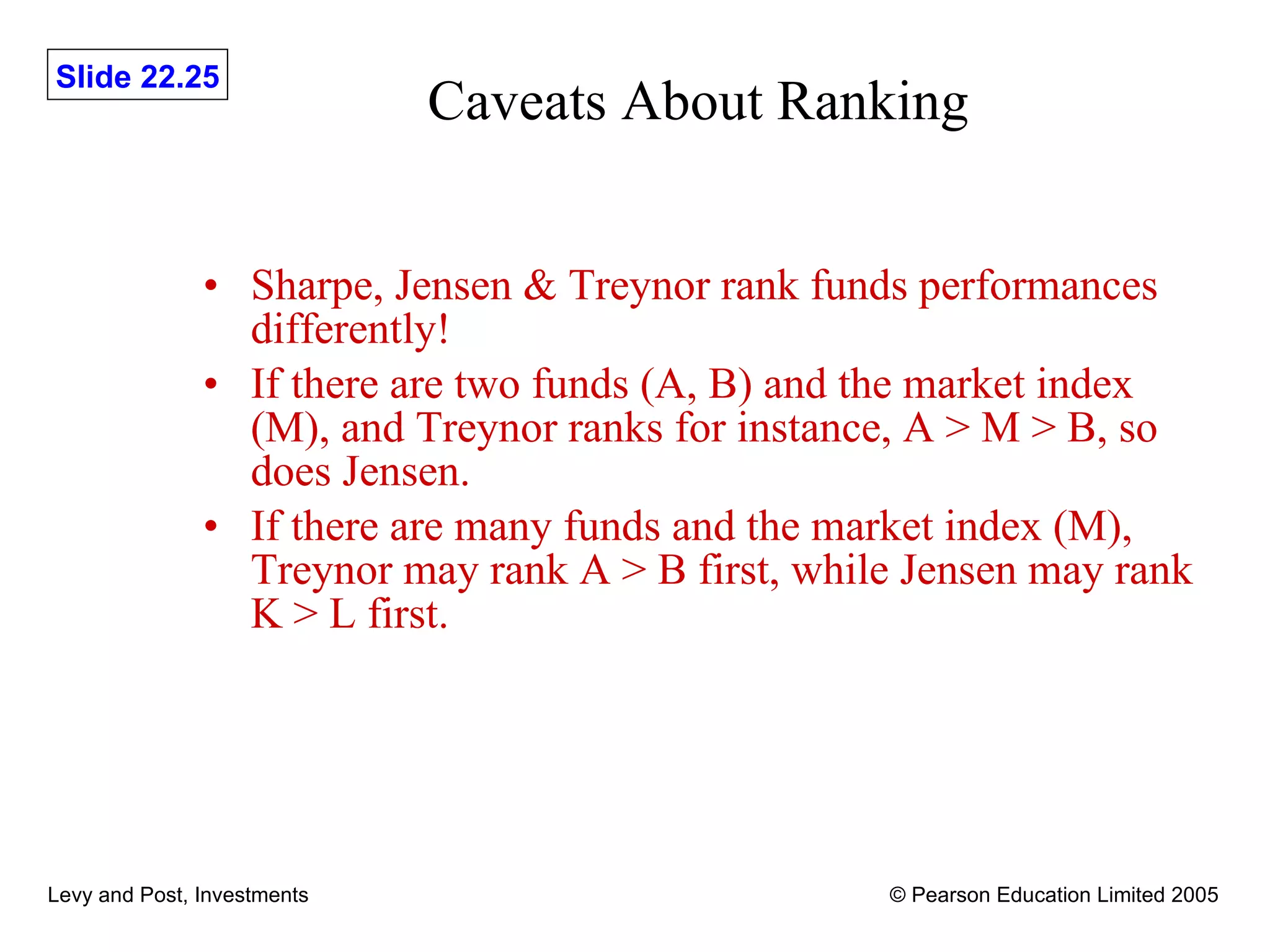
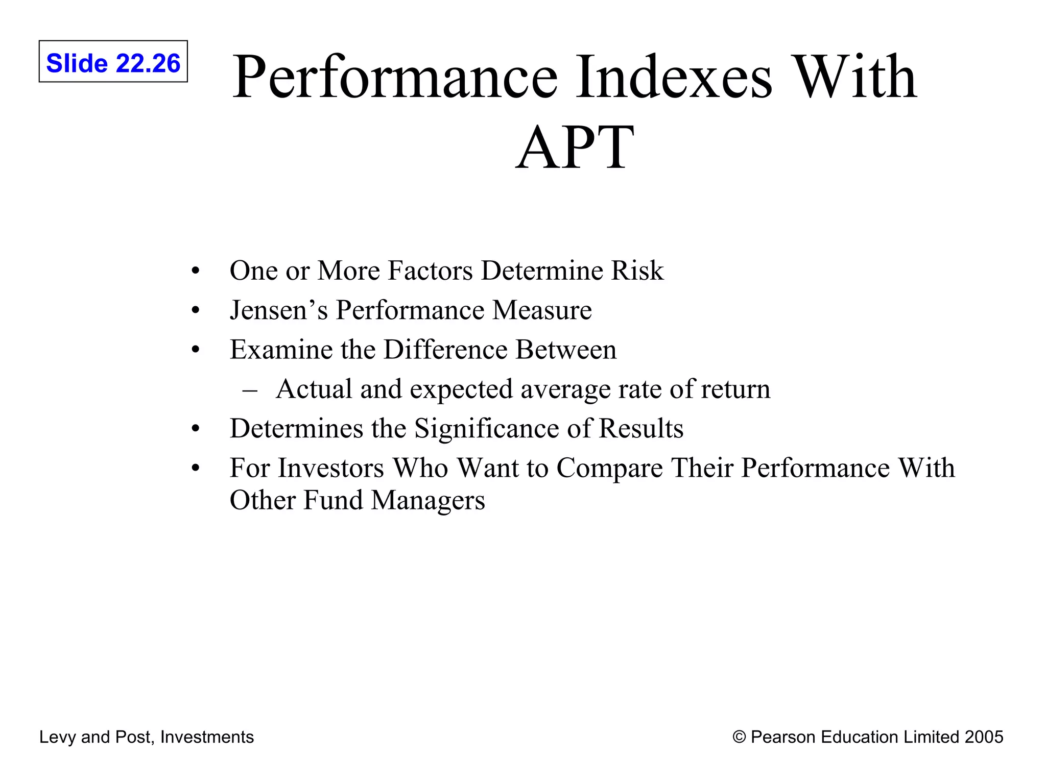
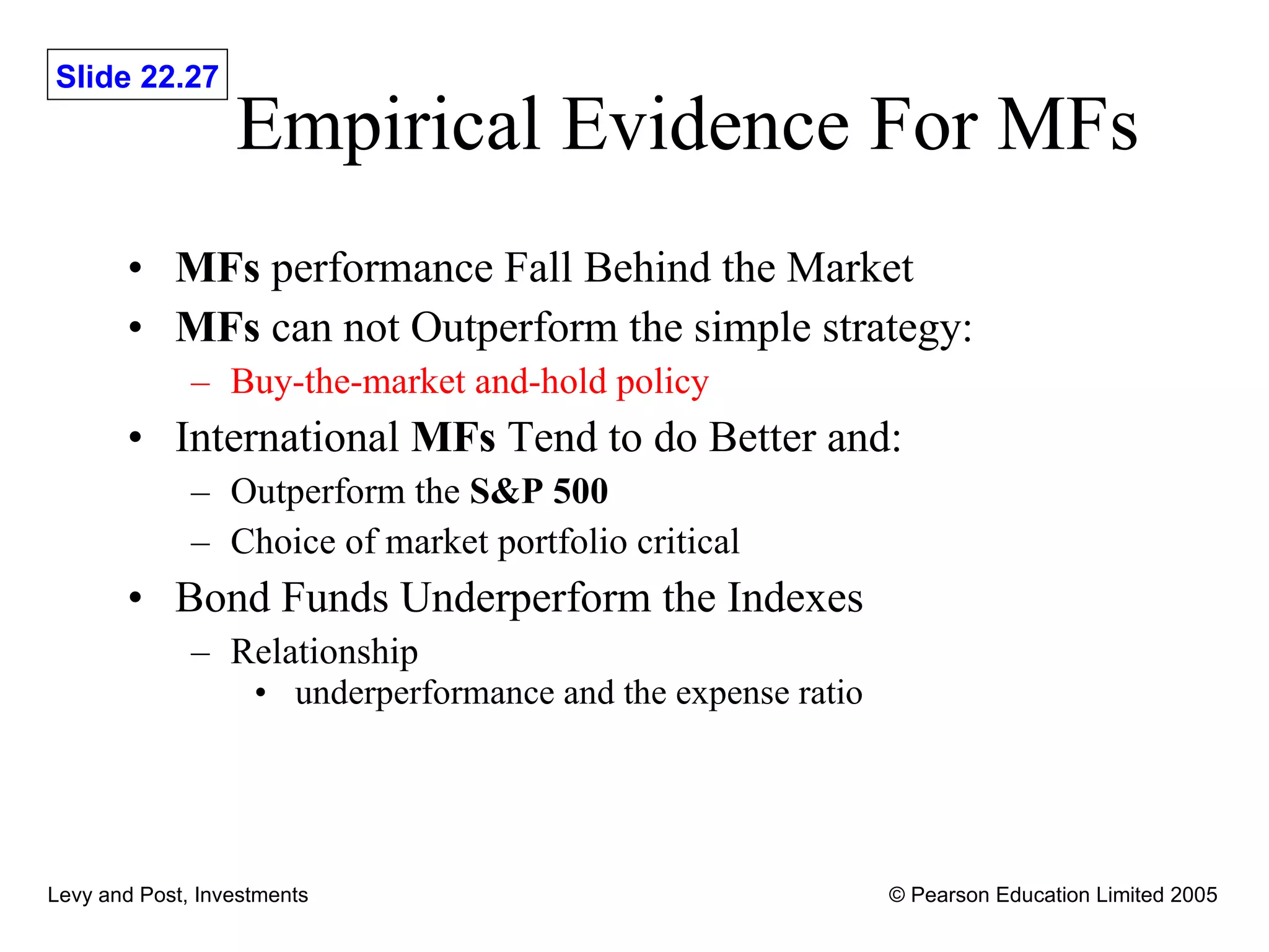
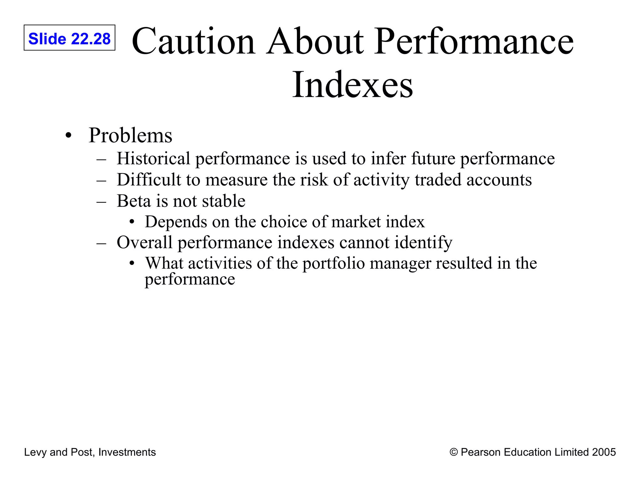
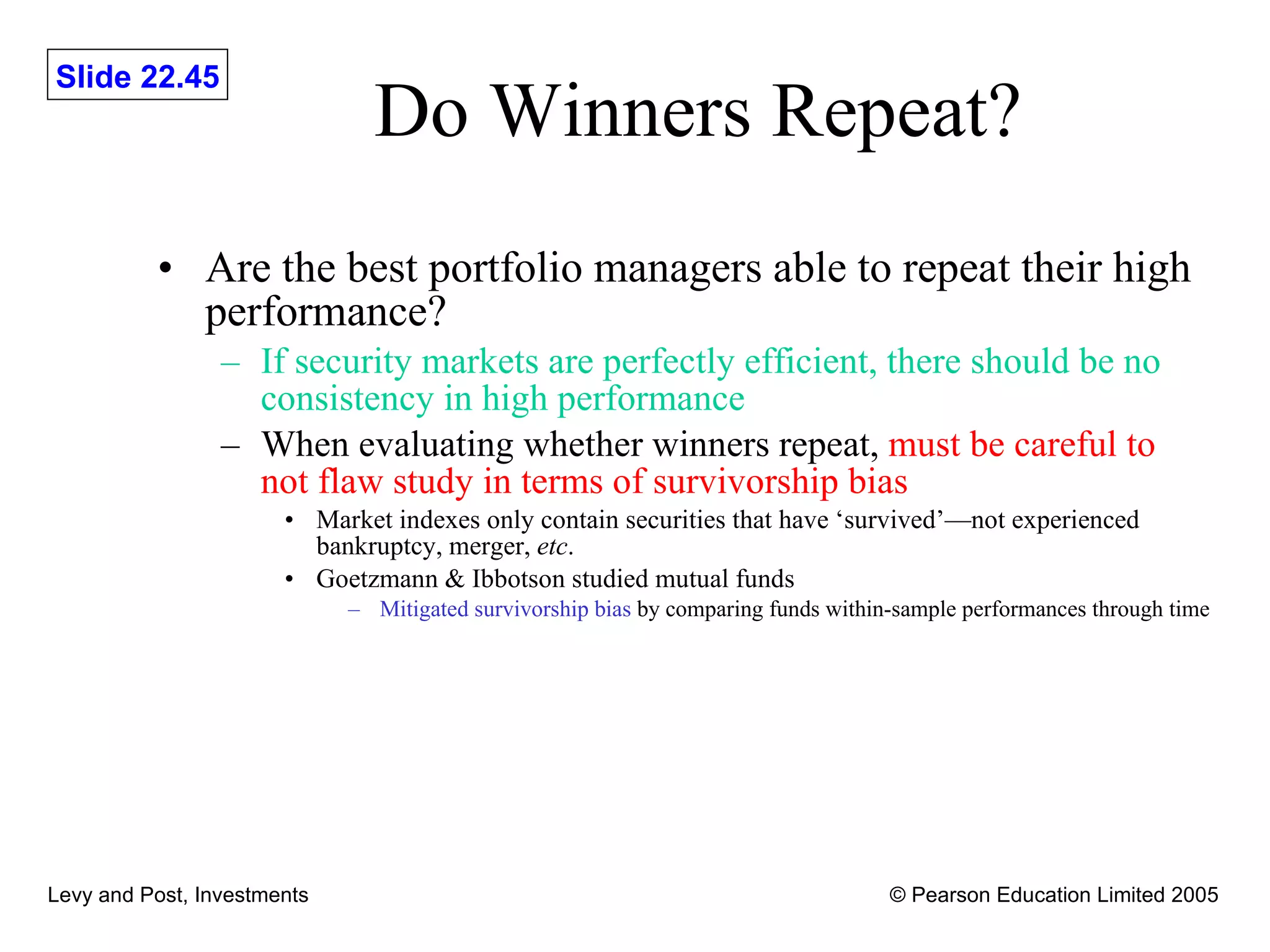
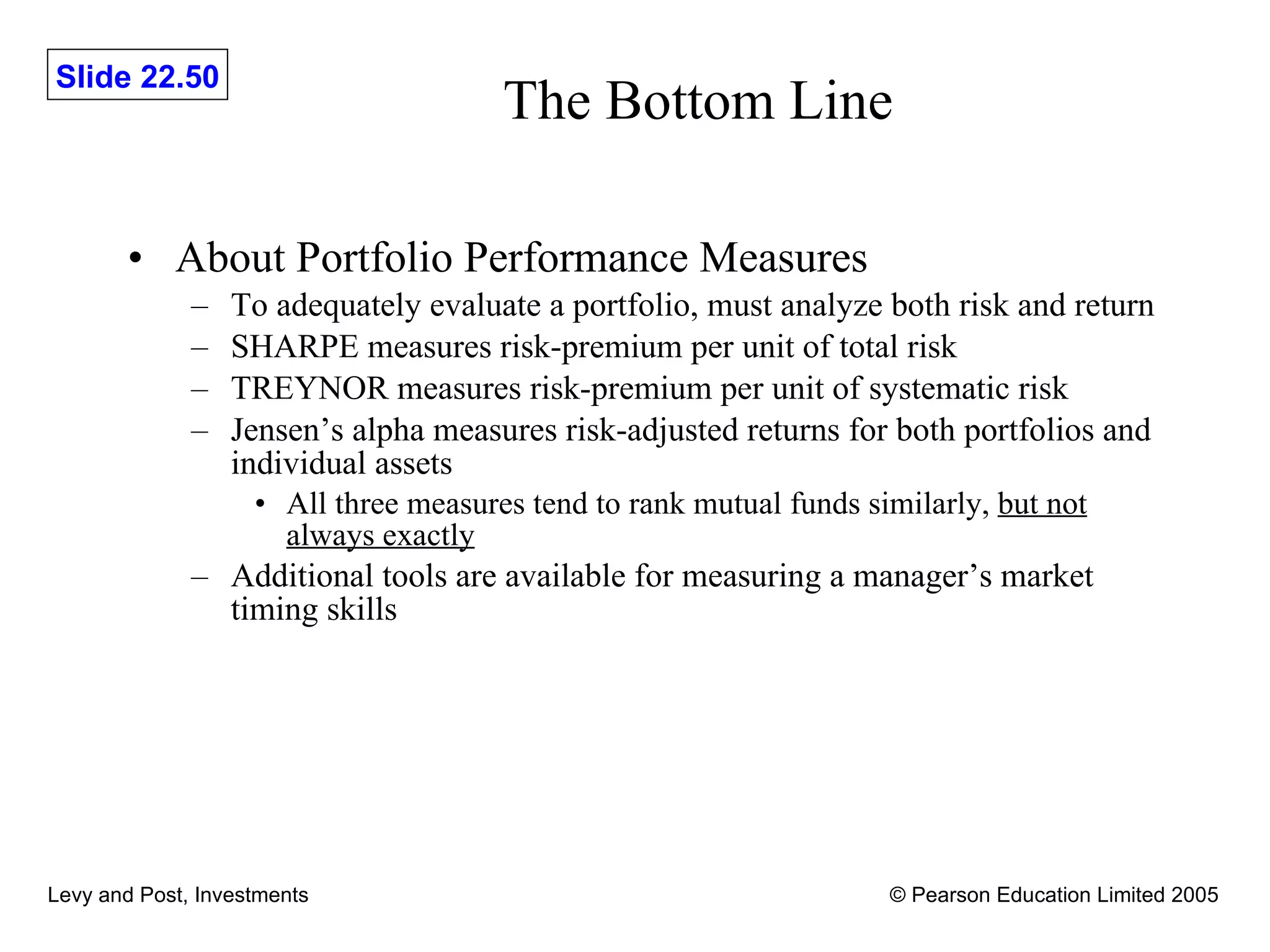
Investments Chapter 22: Performance Evaluation
General Tools for Performance Evaluation Compare performance with risk-adjusted performance indexes. Compare performance against benchmark portfolios. Use of performance attribution methods. Use of comparison universe methods.
How Should Investors Measure Risk? Standard Deviation (absolute risk) Investors with limited holdings Beta (relative risk) Investors with a wide array of holding 12/27/09
Words of Caution when using Performance Evaluation Performance evaluation is an historical exercise while most investors are interested in the future performance of portfolios. Correcting the performance for risk is very difficult. It is very difficult to obtain reliable estimates of the risk and return characteristics of individual securities. The portfolio compositions change over time.
Are Mutual Funds Markowitz Efficient Investments? The mutual funds are all  inefficient investments Funds tend to  group into clusters  corresponding to their investment goals Mutual funds are required to publish written goal statements In a few cases  fund’s stated objective and performance differed   This  income and growth fund  performed in the same league as the  growth funds .
Scrutinizing Mutual Funds Goal Statements Portfolio’s SDs and Betas were better indicators of portfolio’s actual performance than their goal statements.  There are some funds which claim they are growth funds, but get lower return than income funds. # of funds claiming each goal Category’s average rate of return Beta Growth Growth & income Income & Growth Income, Growth & Stability Growth Growth & income Income & Growth Income, Growth & Stability 0.5 to 0.7 3 5 4 16 6.9% 10.1% 9.7% 9.1% 0.7 to 0.9 15 24 7 7 11.2% 10.0% 10.0% 12.2% 0.9 to 1.1 20 1 None 1 13.8% 9.5% None 13.5% Risk Class Range of Betas # of funds Average Beta Average Variance Average Rate of Return Low 0.5 to 0.7 28 0.619 0.000877 9.1% Medium 0.7 to 0.9 53 0.786 0.001543 10.6% High 0.9 to 1.1 22 0.992 0.002304 13.5%
Mutual Fund Performance The empirical evidence finds consistently that mutual fund managers on average lag behind the market if one corrects for risk and costs. Also, there seems to be little consistency in the performance of mutual funds over time.
Risk-adjusted Performance Measures  Sharpe’s Performance Index. Treynor’s Performance Index. Jensen’s Performance Index. APT-based performance measures.
Sharpe’s Performance Index Based on the Slope of the  CML Uses Standard Deviation to Measure Risk (i.e. the interest is to minimize total risk) The Higher the Index, the better the performance Investors Hold Only the Mutual Fund May wish to  rank  portfolios’ performances Need a measure that  includes both risk and return Sharpe measured the  reward to variability index
Sharpe’s Performance Index Based on the CAPM: Where  riskless borrowing and lending is possible at interest rate  r , and where and
Performance Example  (Francis & Ibbotson)   12/27/09 Year Avon Blair Market 1 10.0 10.0 10.0 2 30.0 40.0 30.0 3 -20.0 -20.0 -20.0 4 -10.0 -10.0 -10.0 5 20.0 40.0 20.0 6 10.0 20.0 30.0 7 0.0 -20.0 -10.0 8 30.0 20.0 20.0 9 -10.0 10.0 0.0 10 20.0 40.0 30.0 R 8.0 13.0 10.0  16.6 22.4 17.9  0.8125 1.156 1
SHARPE Example The Avon Fund earned an average return of 8% annually with a standard deviation of 16.6%,   while the Blair Fund earned 13.00% annually with a standard deviation of 22.4%.   During the same time period the average risk-free rate was 4%.  Which fund was the better performer? Since  SHARPE Blair  >  SHARPE Avon , Blair was  the better performer  on a risk-adjusted basis.
SHARPE Example 12/27/09 Avon RFR 13% 8% 22.4% 16.6% Standard Deviation of Returns Expected Return, E(r) Blair Slope is 0.4018 for REVAR Blair Slope is 0.241 for REVAR Avon
Treynor’s Performance Index Based on  SML Uses Beta to measure Risk (i.e. the interest is to minimize the market risk) The Higher the Index, the better the performance Investors Hold Many Assets For Investors Only Interested in Whether They Beat the Market Treynor devised measure to evaluate performance that uses systematic risk (beta) rather than total risk (standard deviation)
Treynor’s Performance Index Based on the APT: Where  riskless borrowing and lending is possible at interest rate  r , and where and
TREYNOR Example The Avon Fund earned an average return of 8% annually (Characteristic Line AVON :  Intercept :  -0.00125;  Beta :  0.8125),   while the Blair Fund earned 13.00% annually (Characteristic Line BLAIR :  Intercept :  0.014;  Beta :  1.156).   During the same time period the average risk-free rate was 4%.  Which fund was the better performer? Since  TREYNOR Blair  >  TREYNOR Avon , Blair was  the better performer  on a risk-adjusted basis.
TREYNOR Example TREYNOR measures the desirability of fund in a SML context Avon RFR 13% 8% 1.156 .8125 Beta Expected Return, E(r) Blair TREYNOR Blair  = 0.0778 TREYNOR Avon  = 0.049 SML
TREYNOR Example Notice that the SML gives slightly different return for both funds! None of them is on the SML! The Avon Fund earned an average return of 8% annually because the Characteristic Line AVON :  -0.00125 + 0.8125*(10% ) +    , where 10% = R m  . According to the SML, the return to Avon Fund is: 4% + 0.8125*(10% - 4%) = 8.875% Similar differences are for the Blair Fund
Jensen’s Alpha Performance Index Based on  CAPM Uses Beta to Measure Risk (equal to the vertical distance to SML) Determines How Much One Fund Outperforms or Underperforms Another Fund (neither Sharpe nor Treynor indicate by how much a fund has outperformed or underperformed the index) Determines the Significance of Results Investors Hold Many Assets
An Investment’s Alpha Jensen modified the characteristic line equation  Rather than using periodic  rates of return , he uses periodic  risk-premiums With expected values (1) gets:
Explanation of an Investment’s Alpha Jensen’s alpha represents excess returns from asset Can be +, 0 or – If asset is  correctly priced, Jensen’s alpha = 0 If  alpha > 0 , asset has earned return greater than appropriate for its level of undiversifiable risk (beta) Asset is  underpriced If  alpha < 0 , asset’s returns are lower than appropriate for its level of risk Asset is  overpriced
Jensen’s Alpha Example Using data ( risk premiums, not returns ) from Table 16-3 (previous slide) for the Avon and Blair Funds: Characteristic Line Avon Jensen’s alpha:  -0.00875 Beta:  0.8125 Characteristic Line Blair Jensen’s alpha:  +0.02062 Beta:  1.1562 Blair earned positive excess returns.
Jensen’s Alpha Example Econometric estimates of (1) Assume actual observations on all funds, market portfolio and risk free returns give the following alpha and beta values: In that case u = 0.03. This is the unik = specific risk of Avon fund
Caveats About Alphas Jensen’s alpha cannot be used to rank performance  of different assets  unless it’s adjusted for the assets’ risks ( same alphas does not imply same performance, because the vertical distance to the SML might be the same, but one fund might have much higher risk )   The  appraisal ratio  divides Jensen’s alpha by the standard error of the estimate (SE (u) ) which then allows for rankings Notice that the alpha = intercept of the original characteristic line (used to estimate our beta) is  not the same as Jensen’s alpha and should not be used for investment performance evaluation
Caveats About Ranking Sharpe, Jensen & Treynor rank funds performances differently! If there are two funds (A, B) and the market index (M), and Treynor ranks for instance, A > M > B, so does Jensen. If there are many funds and the market index (M), Treynor may rank A > B first, while Jensen may rank K > L first.
Performance Indexes With APT One or More Factors Determine Risk Jensen’s Performance Measure Examine the Difference Between  Actual and expected average rate of return Determines the Significance of Results For Investors Who Want to Compare Their Performance With Other Fund Managers
Empirical Evidence For MFs  MFs  performance Fall Behind the Market MFs  can not Outperform the simple strategy: Buy-the-market and-hold policy International  MFs  Tend to do Better and: Outperform the  S&P 500 Choice of market portfolio critical Bond Funds Underperform the Indexes Relationship  underperformance and the expense ratio
Caution About Performance Indexes Problems Historical performance is used to infer future performance Difficult to measure the risk of activity traded accounts Beta is not stable Depends on the choice of market index Overall performance indexes cannot identify What activities of the portfolio manager resulted in the performance
Style Analysis: I An umbrella term for a set of tools for determining the investment style of portfolios and for measuring the performance of portfolios given their investment style.  Money managers are evaluated, in part, based on how well they have offered what they promised or were told to do.
Style Analysis: II Holdings-based Style Analysis Determines the investment style of a portfolio by examining the characteristics of the individual securities in the portfolio. Returns-based Style Analysis Determines the investment style of a portfolio by analyzing its co-movements with indexes that proxy for different styles.
Selection of Money Manager These institutions/individuals must select a money manager This part presents tools for measuring and ranking money managers’ performances Aids in the selection process Money managers also use these tools to appraise and improve their skills
Analyzing a Portfolio Manager’s Style In 1992 Sharpe introduced a model to analyze a portfolio manager’s style ( i.e ., growth vs value investing,  etc .) Uses modest amount of public information about funds Uses price indexes for 12 asset classes as explanatory variables for a mutual fund’s return Sample explanatory factors such as Soloman Brothers 90-day Treasury bill index Lehman Brothers Intermediate-Term Government Bond Index Sharpe/BARRA Value Stock Index
Analyzing a Portfolio Manager’s Style Uses factor analysis The factor loadings are estimates of the weights that a fund invests in the twelve asset categories R 2  of 0.70 are common Sharpe also suggests that same type of analysis could be done using a ‘rolling’ regression Repeating regression when new data is released—dropping oldest data and adding newest data 12/27/09
Performance Attribution The assessment of the performance of portfolio management decisions. Exhibit 22.7   Flow chart of the top-down money-management process Source: From Introduction to Investments, 2nd edn, by Levy.  © 1999. Reprinted with permission of South-Western, a division of Thomson Learning: www.thomsonrights.com. Fax 800 730-2215.
Rolling Style Analysis Ibbotson Associates uses a rolling regression period of 60 months Deleting oldest month and adding new month as data becomes available Some  fixed-income securities  entered this  growth stock  fund in mid 1990s—this is interesting because Magellan’s published investment objective is a growth stock fund.
Benefits From Using Quantitative  Management Style Analysis Quantitative style analysis is important due to: Investment holdings are usually not reported publicly until months after they are made—too late for investors to react in a timely manner Mutual funds can report misleading investment goals Can also provide better forecasts of mutual fund’s risk/return than subjective comments in newspapers,  etc .
Analyzing Performance Statistics Mutual funds with the highest average rate of return might not have the highest rank because A highly aggressive fund may earn higher returns than a less aggressive fund but the higher returns may not be sufficient to compensate for the extra risk taken
Analyzing Performance Statistics While the Yak Fund earned twice as much as the Zebra Fund it is four times as risky. Possible Investments Expected Return Standard Deviation Yak Fund 30% 20% Zebra Fund 15% 5% RFR 4% 0%
Analyzing Performance Statistics By multiplying Zebra’s low SD by 4, we could create a new portfolio on Zebra’s Asset Allocation Line (AAL) with the same high SD as Yak Fund Borrow 4 times as much as the initial equity, invest in Zebra, and achieve the following E(R Zebra ): (4*0.15 - 4*0.04)= 0.48
Analyzing Performance Statistics Check that the SD is the same as for Yak Fund (see notes in SML, the risk free interest rate has zero variance)
Analyzing Performance Statistics The leveraged Zebra portfolio dominates the Yak Fund; thus Zebra is a better fund even though Yak has a higher average return. Perhaps both Treynor and Jensen would give the same ranking in this case Yak RFR 48% 30% 20% 5% Standard Deviation Expected Return, E(r) Zebra Zebra’s SHARPE = 2.2 Yak’s SHARPE = 1.3 15% Yak’s AAL Zebra’s AAL
General Discussion of Performance Measurement Tools When investors analyze merits of alternative investments, usually concerned with Asset selection Portfolio manager’s ability to select good investments and to not select poor investments Sharpe, Treynor & Jensen’s Alpha are good tools to evaluate this issue Market timing Portfolio manager’s ability to buy low/sell high and manager’s ability to react to changes in market’s direction Sharpe, Treynor & Jensen’s Alpha are not good tools for evaluating market timing unless theoretical framework is extended
Evaluating Timing Decisions Treynor & Mazuy included a second-order term in the characteristic line to evaluate market-timing
Evaluating Timing Decisions A successful market timer will Shift into  high beta securities  when  bull market begins Shift into  low beta securities  when  bear market begins If portfolio manager does this, beta 2,investment  > 0 If portfolio manager cannot outguess market turns, beta 2,investment  = 0 (statistically) If portfolio manager incorrectly predicts market turns, beta 2,investment  < 0   12/27/09
Do Winners Repeat? Are the best portfolio managers able to repeat their high performance? If security markets are perfectly efficient, there should be no consistency in high performance When evaluating whether winners repeat,  must be careful to not flaw study in terms of survivorship bias Market indexes only contain securities that have ‘survived’—not experienced bankruptcy, merger,  etc . Goetzmann & Ibbotson studied mutual funds Mitigated survivorship bias  by comparing funds within-sample performances through time
Goetzmann & Ibbotson Study Database Monthly total returns of several hundred mutual funds over a 13-year period Management fees deducted, but load, exit fees and taxes were not considered All cash flows reinvested monthly Returns measured over 2-year within-sample period, beginning in 1976 to predict out-of-sample performance for subsequent 2-year period Only funds in existence for entire 2-year interval included Every mutual fund categorized as ‘winner’ or ‘loser’ based on whether it ranked above or below that 2-year sample’s median return
Goetzmann & Ibbotson Study The combined results show that there is about a 60% chance a winner will be a winner the following period. But, the repeat-winners pattern didn’t persist during this subsample. 1978-1979 Winners 1978-1979 Losers 1980-1981 Winners 1980-1981 Losers 1976-1977 Winners 84 54 1978-1979 Winners 110 41 1976-1977 Losers 50 88 1978-1979 Losers 38 113 1982-1983 Winners 1982-1983  Losers 1984-1985 Winners 1984-1985 Losers 1980-1981 Winners 63 96 1982-1983 Winners 104 62 1980-1981 Losers 96 63 1982-1983 Losers 71 95 Combined Results Successive Period 1986-1987 Winners 1986-1987 Losers Winners Losers 1984-1985 Winners 125 72 Initial  Winners 486 59.9% 325 40.1% 1984-1985 Losers 72 125 Initial Losers 327 40.3% 484 59.7%
Goetzmann & Ibbotson Study However, these high-return mutual funds  could continue to have high-ranking returns due to high risk, not because they were winners G&I replicate study using  risk-adjusted returns Computed Jensen’s Alpha for each fund Classified fund as a winner or loser if fund’s alpha > or < period’s median alpha Results show that  winners tend to repeat in all 5 subsamples Also , divided sample into growth funds  and found similar results Also,  used 1-year subsamples  rather than 2-year Similar, but weaker, support for the repeat winners hypothesis
Other Studies Malkiel argues that while  repeat winners phenomenon existed in 1970s, it was not present during 1980s Carhart finds that  winning funds tend to have a winning performance the following year, but not afterwards Losers have a strong tendency to persist  with the worst performers persisting for years
The Bottom Line About Portfolio Performance Measures To adequately evaluate a portfolio, must analyze both risk and return SHARPE measures risk-premium per unit of total risk TREYNOR measures risk-premium per unit of systematic risk Jensen’s alpha measures risk-adjusted returns for both portfolios and individual assets All three measures tend to rank mutual funds similarly,  but not always exactly Additional tools are available for measuring a manager’s market timing skills
The Bottom Line About mutual fund investments Average American buying round lots can afford only about 7 different stocks Not enough to minimize diversifiable risk Mutual funds  are usually  able to reduce their diversifiable risk Investors can maintain their desired risk-class  by mutual fund investing Most investors should  focus on a mutual fund’s fees  and favor funds charging smallest fees

L Pch22

  • 1.
    Investments Chapter 22:Performance Evaluation
  • 2.
    General Tools forPerformance Evaluation Compare performance with risk-adjusted performance indexes. Compare performance against benchmark portfolios. Use of performance attribution methods. Use of comparison universe methods.
  • 3.
    How Should InvestorsMeasure Risk? Standard Deviation (absolute risk) Investors with limited holdings Beta (relative risk) Investors with a wide array of holding 12/27/09
  • 4.
    Words of Cautionwhen using Performance Evaluation Performance evaluation is an historical exercise while most investors are interested in the future performance of portfolios. Correcting the performance for risk is very difficult. It is very difficult to obtain reliable estimates of the risk and return characteristics of individual securities. The portfolio compositions change over time.
  • 5.
    Are Mutual FundsMarkowitz Efficient Investments? The mutual funds are all inefficient investments Funds tend to group into clusters corresponding to their investment goals Mutual funds are required to publish written goal statements In a few cases fund’s stated objective and performance differed This income and growth fund performed in the same league as the growth funds .
  • 6.
    Scrutinizing Mutual FundsGoal Statements Portfolio’s SDs and Betas were better indicators of portfolio’s actual performance than their goal statements. There are some funds which claim they are growth funds, but get lower return than income funds. # of funds claiming each goal Category’s average rate of return Beta Growth Growth & income Income & Growth Income, Growth & Stability Growth Growth & income Income & Growth Income, Growth & Stability 0.5 to 0.7 3 5 4 16 6.9% 10.1% 9.7% 9.1% 0.7 to 0.9 15 24 7 7 11.2% 10.0% 10.0% 12.2% 0.9 to 1.1 20 1 None 1 13.8% 9.5% None 13.5% Risk Class Range of Betas # of funds Average Beta Average Variance Average Rate of Return Low 0.5 to 0.7 28 0.619 0.000877 9.1% Medium 0.7 to 0.9 53 0.786 0.001543 10.6% High 0.9 to 1.1 22 0.992 0.002304 13.5%
  • 7.
    Mutual Fund PerformanceThe empirical evidence finds consistently that mutual fund managers on average lag behind the market if one corrects for risk and costs. Also, there seems to be little consistency in the performance of mutual funds over time.
  • 8.
    Risk-adjusted Performance Measures Sharpe’s Performance Index. Treynor’s Performance Index. Jensen’s Performance Index. APT-based performance measures.
  • 9.
    Sharpe’s Performance IndexBased on the Slope of the CML Uses Standard Deviation to Measure Risk (i.e. the interest is to minimize total risk) The Higher the Index, the better the performance Investors Hold Only the Mutual Fund May wish to rank portfolios’ performances Need a measure that includes both risk and return Sharpe measured the reward to variability index
  • 10.
    Sharpe’s Performance IndexBased on the CAPM: Where riskless borrowing and lending is possible at interest rate r , and where and
  • 11.
    Performance Example (Francis & Ibbotson) 12/27/09 Year Avon Blair Market 1 10.0 10.0 10.0 2 30.0 40.0 30.0 3 -20.0 -20.0 -20.0 4 -10.0 -10.0 -10.0 5 20.0 40.0 20.0 6 10.0 20.0 30.0 7 0.0 -20.0 -10.0 8 30.0 20.0 20.0 9 -10.0 10.0 0.0 10 20.0 40.0 30.0 R 8.0 13.0 10.0  16.6 22.4 17.9  0.8125 1.156 1
  • 12.
    SHARPE Example TheAvon Fund earned an average return of 8% annually with a standard deviation of 16.6%, while the Blair Fund earned 13.00% annually with a standard deviation of 22.4%. During the same time period the average risk-free rate was 4%. Which fund was the better performer? Since SHARPE Blair > SHARPE Avon , Blair was the better performer on a risk-adjusted basis.
  • 13.
    SHARPE Example 12/27/09Avon RFR 13% 8% 22.4% 16.6% Standard Deviation of Returns Expected Return, E(r) Blair Slope is 0.4018 for REVAR Blair Slope is 0.241 for REVAR Avon
  • 14.
    Treynor’s Performance IndexBased on SML Uses Beta to measure Risk (i.e. the interest is to minimize the market risk) The Higher the Index, the better the performance Investors Hold Many Assets For Investors Only Interested in Whether They Beat the Market Treynor devised measure to evaluate performance that uses systematic risk (beta) rather than total risk (standard deviation)
  • 15.
    Treynor’s Performance IndexBased on the APT: Where riskless borrowing and lending is possible at interest rate r , and where and
  • 16.
    TREYNOR Example TheAvon Fund earned an average return of 8% annually (Characteristic Line AVON : Intercept : -0.00125; Beta : 0.8125), while the Blair Fund earned 13.00% annually (Characteristic Line BLAIR : Intercept : 0.014; Beta : 1.156). During the same time period the average risk-free rate was 4%. Which fund was the better performer? Since TREYNOR Blair > TREYNOR Avon , Blair was the better performer on a risk-adjusted basis.
  • 17.
    TREYNOR Example TREYNORmeasures the desirability of fund in a SML context Avon RFR 13% 8% 1.156 .8125 Beta Expected Return, E(r) Blair TREYNOR Blair = 0.0778 TREYNOR Avon = 0.049 SML
  • 18.
    TREYNOR Example Noticethat the SML gives slightly different return for both funds! None of them is on the SML! The Avon Fund earned an average return of 8% annually because the Characteristic Line AVON : -0.00125 + 0.8125*(10% ) +  , where 10% = R m . According to the SML, the return to Avon Fund is: 4% + 0.8125*(10% - 4%) = 8.875% Similar differences are for the Blair Fund
  • 19.
    Jensen’s Alpha PerformanceIndex Based on CAPM Uses Beta to Measure Risk (equal to the vertical distance to SML) Determines How Much One Fund Outperforms or Underperforms Another Fund (neither Sharpe nor Treynor indicate by how much a fund has outperformed or underperformed the index) Determines the Significance of Results Investors Hold Many Assets
  • 20.
    An Investment’s AlphaJensen modified the characteristic line equation Rather than using periodic rates of return , he uses periodic risk-premiums With expected values (1) gets:
  • 21.
    Explanation of anInvestment’s Alpha Jensen’s alpha represents excess returns from asset Can be +, 0 or – If asset is correctly priced, Jensen’s alpha = 0 If alpha > 0 , asset has earned return greater than appropriate for its level of undiversifiable risk (beta) Asset is underpriced If alpha < 0 , asset’s returns are lower than appropriate for its level of risk Asset is overpriced
  • 22.
    Jensen’s Alpha ExampleUsing data ( risk premiums, not returns ) from Table 16-3 (previous slide) for the Avon and Blair Funds: Characteristic Line Avon Jensen’s alpha: -0.00875 Beta: 0.8125 Characteristic Line Blair Jensen’s alpha: +0.02062 Beta: 1.1562 Blair earned positive excess returns.
  • 23.
    Jensen’s Alpha ExampleEconometric estimates of (1) Assume actual observations on all funds, market portfolio and risk free returns give the following alpha and beta values: In that case u = 0.03. This is the unik = specific risk of Avon fund
  • 24.
    Caveats About AlphasJensen’s alpha cannot be used to rank performance of different assets unless it’s adjusted for the assets’ risks ( same alphas does not imply same performance, because the vertical distance to the SML might be the same, but one fund might have much higher risk ) The appraisal ratio divides Jensen’s alpha by the standard error of the estimate (SE (u) ) which then allows for rankings Notice that the alpha = intercept of the original characteristic line (used to estimate our beta) is not the same as Jensen’s alpha and should not be used for investment performance evaluation
  • 25.
    Caveats About RankingSharpe, Jensen & Treynor rank funds performances differently! If there are two funds (A, B) and the market index (M), and Treynor ranks for instance, A > M > B, so does Jensen. If there are many funds and the market index (M), Treynor may rank A > B first, while Jensen may rank K > L first.
  • 26.
    Performance Indexes WithAPT One or More Factors Determine Risk Jensen’s Performance Measure Examine the Difference Between Actual and expected average rate of return Determines the Significance of Results For Investors Who Want to Compare Their Performance With Other Fund Managers
  • 27.
    Empirical Evidence ForMFs MFs performance Fall Behind the Market MFs can not Outperform the simple strategy: Buy-the-market and-hold policy International MFs Tend to do Better and: Outperform the S&P 500 Choice of market portfolio critical Bond Funds Underperform the Indexes Relationship underperformance and the expense ratio
  • 28.
    Caution About PerformanceIndexes Problems Historical performance is used to infer future performance Difficult to measure the risk of activity traded accounts Beta is not stable Depends on the choice of market index Overall performance indexes cannot identify What activities of the portfolio manager resulted in the performance
  • 29.
    Style Analysis: IAn umbrella term for a set of tools for determining the investment style of portfolios and for measuring the performance of portfolios given their investment style. Money managers are evaluated, in part, based on how well they have offered what they promised or were told to do.
  • 30.
    Style Analysis: IIHoldings-based Style Analysis Determines the investment style of a portfolio by examining the characteristics of the individual securities in the portfolio. Returns-based Style Analysis Determines the investment style of a portfolio by analyzing its co-movements with indexes that proxy for different styles.
  • 31.
    Selection of MoneyManager These institutions/individuals must select a money manager This part presents tools for measuring and ranking money managers’ performances Aids in the selection process Money managers also use these tools to appraise and improve their skills
  • 32.
    Analyzing a PortfolioManager’s Style In 1992 Sharpe introduced a model to analyze a portfolio manager’s style ( i.e ., growth vs value investing, etc .) Uses modest amount of public information about funds Uses price indexes for 12 asset classes as explanatory variables for a mutual fund’s return Sample explanatory factors such as Soloman Brothers 90-day Treasury bill index Lehman Brothers Intermediate-Term Government Bond Index Sharpe/BARRA Value Stock Index
  • 33.
    Analyzing a PortfolioManager’s Style Uses factor analysis The factor loadings are estimates of the weights that a fund invests in the twelve asset categories R 2 of 0.70 are common Sharpe also suggests that same type of analysis could be done using a ‘rolling’ regression Repeating regression when new data is released—dropping oldest data and adding newest data 12/27/09
  • 34.
    Performance Attribution Theassessment of the performance of portfolio management decisions. Exhibit 22.7 Flow chart of the top-down money-management process Source: From Introduction to Investments, 2nd edn, by Levy. © 1999. Reprinted with permission of South-Western, a division of Thomson Learning: www.thomsonrights.com. Fax 800 730-2215.
  • 35.
    Rolling Style AnalysisIbbotson Associates uses a rolling regression period of 60 months Deleting oldest month and adding new month as data becomes available Some fixed-income securities entered this growth stock fund in mid 1990s—this is interesting because Magellan’s published investment objective is a growth stock fund.
  • 36.
    Benefits From UsingQuantitative Management Style Analysis Quantitative style analysis is important due to: Investment holdings are usually not reported publicly until months after they are made—too late for investors to react in a timely manner Mutual funds can report misleading investment goals Can also provide better forecasts of mutual fund’s risk/return than subjective comments in newspapers, etc .
  • 37.
    Analyzing Performance StatisticsMutual funds with the highest average rate of return might not have the highest rank because A highly aggressive fund may earn higher returns than a less aggressive fund but the higher returns may not be sufficient to compensate for the extra risk taken
  • 38.
    Analyzing Performance StatisticsWhile the Yak Fund earned twice as much as the Zebra Fund it is four times as risky. Possible Investments Expected Return Standard Deviation Yak Fund 30% 20% Zebra Fund 15% 5% RFR 4% 0%
  • 39.
    Analyzing Performance StatisticsBy multiplying Zebra’s low SD by 4, we could create a new portfolio on Zebra’s Asset Allocation Line (AAL) with the same high SD as Yak Fund Borrow 4 times as much as the initial equity, invest in Zebra, and achieve the following E(R Zebra ): (4*0.15 - 4*0.04)= 0.48
  • 40.
    Analyzing Performance StatisticsCheck that the SD is the same as for Yak Fund (see notes in SML, the risk free interest rate has zero variance)
  • 41.
    Analyzing Performance StatisticsThe leveraged Zebra portfolio dominates the Yak Fund; thus Zebra is a better fund even though Yak has a higher average return. Perhaps both Treynor and Jensen would give the same ranking in this case Yak RFR 48% 30% 20% 5% Standard Deviation Expected Return, E(r) Zebra Zebra’s SHARPE = 2.2 Yak’s SHARPE = 1.3 15% Yak’s AAL Zebra’s AAL
  • 42.
    General Discussion ofPerformance Measurement Tools When investors analyze merits of alternative investments, usually concerned with Asset selection Portfolio manager’s ability to select good investments and to not select poor investments Sharpe, Treynor & Jensen’s Alpha are good tools to evaluate this issue Market timing Portfolio manager’s ability to buy low/sell high and manager’s ability to react to changes in market’s direction Sharpe, Treynor & Jensen’s Alpha are not good tools for evaluating market timing unless theoretical framework is extended
  • 43.
    Evaluating Timing DecisionsTreynor & Mazuy included a second-order term in the characteristic line to evaluate market-timing
  • 44.
    Evaluating Timing DecisionsA successful market timer will Shift into high beta securities when bull market begins Shift into low beta securities when bear market begins If portfolio manager does this, beta 2,investment > 0 If portfolio manager cannot outguess market turns, beta 2,investment = 0 (statistically) If portfolio manager incorrectly predicts market turns, beta 2,investment < 0 12/27/09
  • 45.
    Do Winners Repeat?Are the best portfolio managers able to repeat their high performance? If security markets are perfectly efficient, there should be no consistency in high performance When evaluating whether winners repeat, must be careful to not flaw study in terms of survivorship bias Market indexes only contain securities that have ‘survived’—not experienced bankruptcy, merger, etc . Goetzmann & Ibbotson studied mutual funds Mitigated survivorship bias by comparing funds within-sample performances through time
  • 46.
    Goetzmann & IbbotsonStudy Database Monthly total returns of several hundred mutual funds over a 13-year period Management fees deducted, but load, exit fees and taxes were not considered All cash flows reinvested monthly Returns measured over 2-year within-sample period, beginning in 1976 to predict out-of-sample performance for subsequent 2-year period Only funds in existence for entire 2-year interval included Every mutual fund categorized as ‘winner’ or ‘loser’ based on whether it ranked above or below that 2-year sample’s median return
  • 47.
    Goetzmann & IbbotsonStudy The combined results show that there is about a 60% chance a winner will be a winner the following period. But, the repeat-winners pattern didn’t persist during this subsample. 1978-1979 Winners 1978-1979 Losers 1980-1981 Winners 1980-1981 Losers 1976-1977 Winners 84 54 1978-1979 Winners 110 41 1976-1977 Losers 50 88 1978-1979 Losers 38 113 1982-1983 Winners 1982-1983 Losers 1984-1985 Winners 1984-1985 Losers 1980-1981 Winners 63 96 1982-1983 Winners 104 62 1980-1981 Losers 96 63 1982-1983 Losers 71 95 Combined Results Successive Period 1986-1987 Winners 1986-1987 Losers Winners Losers 1984-1985 Winners 125 72 Initial Winners 486 59.9% 325 40.1% 1984-1985 Losers 72 125 Initial Losers 327 40.3% 484 59.7%
  • 48.
    Goetzmann & IbbotsonStudy However, these high-return mutual funds could continue to have high-ranking returns due to high risk, not because they were winners G&I replicate study using risk-adjusted returns Computed Jensen’s Alpha for each fund Classified fund as a winner or loser if fund’s alpha > or < period’s median alpha Results show that winners tend to repeat in all 5 subsamples Also , divided sample into growth funds and found similar results Also, used 1-year subsamples rather than 2-year Similar, but weaker, support for the repeat winners hypothesis
  • 49.
    Other Studies Malkielargues that while repeat winners phenomenon existed in 1970s, it was not present during 1980s Carhart finds that winning funds tend to have a winning performance the following year, but not afterwards Losers have a strong tendency to persist with the worst performers persisting for years
  • 50.
    The Bottom LineAbout Portfolio Performance Measures To adequately evaluate a portfolio, must analyze both risk and return SHARPE measures risk-premium per unit of total risk TREYNOR measures risk-premium per unit of systematic risk Jensen’s alpha measures risk-adjusted returns for both portfolios and individual assets All three measures tend to rank mutual funds similarly, but not always exactly Additional tools are available for measuring a manager’s market timing skills
  • 51.
    The Bottom LineAbout mutual fund investments Average American buying round lots can afford only about 7 different stocks Not enough to minimize diversifiable risk Mutual funds are usually able to reduce their diversifiable risk Investors can maintain their desired risk-class by mutual fund investing Most investors should focus on a mutual fund’s fees and favor funds charging smallest fees