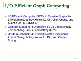
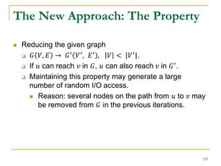
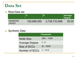
Downloaded 14 times


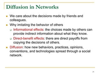
![An Existing Approach
MB [Mishra and Bhattacharya, WWW’11]
The trustworthiness of a user cannot be trusted,
because MB treats the bias of a user by relative
differences between itself and others.
If a user gives all his/her friends a much higher trust
score than the average of others, and gives all his/her
foes a much lower trust score than the average of
others, such differences cancel out. This user has
zero bias and can be 100% trusted.
21](https://image.slidesharecdn.com/jeffreyxuyu-largegraphprocessing-160616082809/85/Jeffrey-xu-yu-large-graph-processing-21-320.jpg)
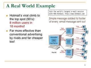
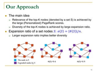
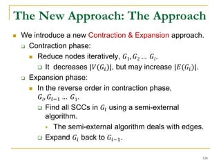
![Our Approach
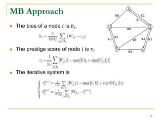
We use two vectors, 𝑏 and 𝑟, for bias and prestige.
The 𝑏𝑗 = (𝑓(𝑟)) 𝑗 denotes the bias of node 𝑗, where 𝑟 is
the prestige vector of the nodes, and 𝑓(𝑟) is a vector-
valued contractive function. (𝑓 𝑟 ) 𝑗 denotes the 𝑗-th
element of vector 𝑓(𝑟).
Let 0 ≤ 𝑓(𝑟) ≤ 𝑒, and 𝑒 = [1, 1, … , 1] 𝑇
For any 𝑥, 𝑦 ∈ 𝑅 𝑛, the function 𝑓: 𝑅 𝑛 → 𝑅 𝑛 is a vector-
valued contractive function if the following condition
holds,
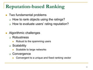
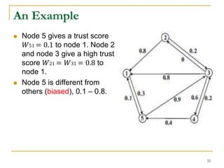
𝑓 𝑥 – 𝑓 𝑦 ≤ 𝜆 ∥ 𝑥 − 𝑦 ∥∞ 𝑒
where 𝜆 ∈ [0,1) and ∥∙∥∞ denotes the infinity norm.
26](https://image.slidesharecdn.com/jeffreyxuyu-largegraphprocessing-160616082809/85/Jeffrey-xu-yu-large-graph-processing-26-320.jpg)

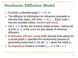
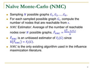
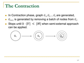
![Naïve Monte-Carlo (NMC)
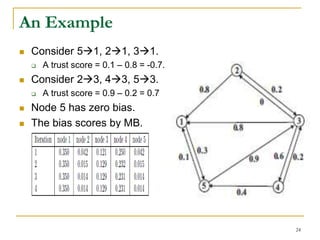
In practice, it resorts to an unbiased estimator of 𝑉𝑎𝑟( 𝐹 𝑁𝑀𝐶).
The variance of 𝑁𝑀𝐶 is
𝑉𝑎𝑟 𝐹 𝑁𝑀𝐶 =
𝑖=1
𝑁
(𝑓𝑠 𝐺𝑖 − 𝐹 𝑁𝑀𝐶)2
𝑁 − 1
But, 𝑉𝑎𝑟 𝐹 𝑁𝑀𝐶 may be very large, because 𝑓𝑠 𝐺𝑖 fall into
the interval [0, 𝑛 − 1].
The variance can be up to 𝑂(𝑛2).
43](https://image.slidesharecdn.com/jeffreyxuyu-largegraphprocessing-160616082809/85/Jeffrey-xu-yu-large-graph-processing-43-320.jpg)
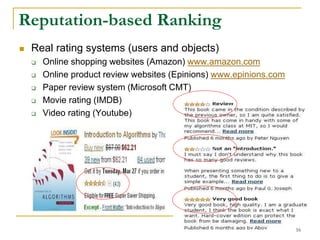
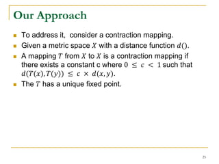
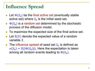
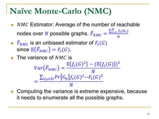
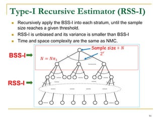
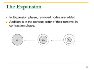
![A Recursive Estimator [Jin et al. VLDB’11]
Randomly select 1 edge to partition the probability
space (the set of all possible graphs) into 2 strata
(2 subsets)
The possible graphs in the first subset include
the selected edge.
The possible graphs in the second subset do
not include the selected edge.
Sample possible graphs in each stratum 𝑖 with a
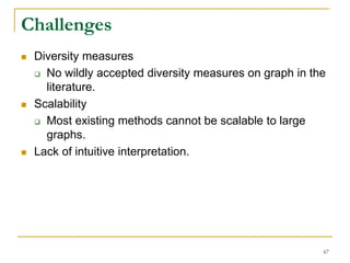
sample size 𝑁𝑖 proportioning to the probability of
that stratum.
Recursively apply the same idea in each stratum.
45](https://image.slidesharecdn.com/jeffreyxuyu-largegraphprocessing-160616082809/85/Jeffrey-xu-yu-large-graph-processing-45-320.jpg)
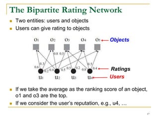
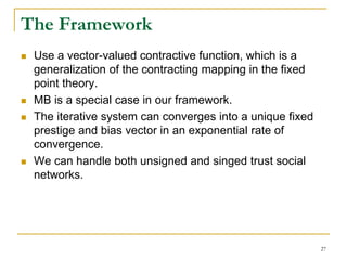
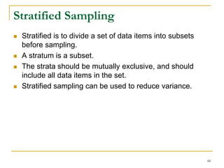
![A Recursive Estimator [Jin et al. VLDB’11]
Advantages:
unbiased estimator with a smaller variance.
Limitations:
Select only one edge for stratification, which is not
enough to significantly reduce the variance.
Randomly select edges, which results in a possible
large variance.
46](https://image.slidesharecdn.com/jeffreyxuyu-largegraphprocessing-160616082809/85/Jeffrey-xu-yu-large-graph-processing-46-320.jpg)
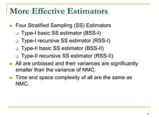
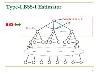
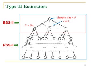
![Type-I Basic Estimator (BSS-I)
Select 𝑟 edges to partition the probability space (all the
possible graphs) into 2 𝑟
strata.
Each stratum corresponds to a probability subspace
(a set of possible graphs).
Let 𝜋𝑖 = Pr[𝐺 𝑃 ∈ Ω𝑖].
How to select 𝑟 edges: BFS or random
48](https://image.slidesharecdn.com/jeffreyxuyu-largegraphprocessing-160616082809/85/Jeffrey-xu-yu-large-graph-processing-48-320.jpg)
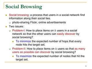
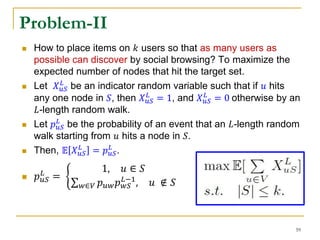
![ The two problems are a random walk problem.
𝐿-length random walk model where the path length of
random walks is bounded by a nonnegative number 𝐿.
A random walk in general can be considered as 𝐿 = ∞.
Let 𝑍 𝑢
𝑡
be the position of an 𝐿-length random walk,
starting from node 𝑢, at discrete time 𝑡.
Let 𝑇𝑢𝑣
𝐿 be a random walk variable.
𝑇𝑢𝑣
𝐿
≜ min{min 𝑡: 𝑍 𝑢
𝑡
= v, t ≥ 0}, 𝐿
The hitting time ℎ 𝑢𝑣
𝐿 can be defined as the expectation
of 𝑇𝑢𝑣
𝐿 .
ℎ 𝑢𝑣
𝐿
= 𝔼[𝑇𝑢𝑣
𝐿
]
The Random Walk
55](https://image.slidesharecdn.com/jeffreyxuyu-largegraphprocessing-160616082809/85/Jeffrey-xu-yu-large-graph-processing-55-320.jpg)
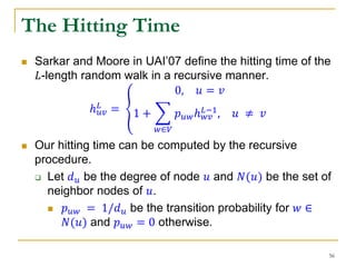
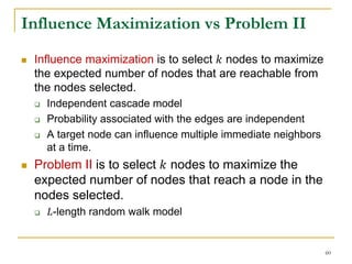
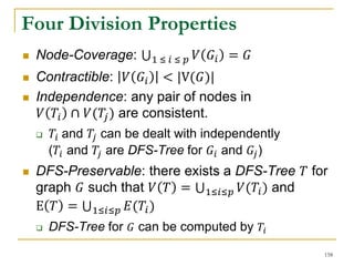
![The Random-Walk Domination
Consider a set of nodes 𝑆. If a random walk from 𝑢
reaches 𝑆 by an 𝐿-length random walk, we say
𝑆 dominates 𝑢 by an 𝐿-length random walk.
Generalized hitting time over a set of nodes, 𝑆. The
hitting time ℎ 𝑢𝑆
𝐿
can be defined as the expectation of a
random walk variable 𝑇𝑢𝑆
𝐿
.
𝑇𝑢𝑆
𝐿
≜ min{min 𝑡: 𝑍 𝑢
𝑡
∈ 𝑆, t ≥ 0}, 𝐿
ℎ 𝑢𝑆
𝐿
= 𝔼[𝑇𝑢𝑆
𝐿
]
It can be computed recursively.
ℎ 𝑢𝑆
𝐿
=
0, 𝑢 ∈ 𝑆
1 + 𝑤∈𝑉 𝑝 𝑢𝑤ℎ 𝑤𝑆
𝐿−1
, 𝑢 ∉ 𝑆
57](https://image.slidesharecdn.com/jeffreyxuyu-largegraphprocessing-160616082809/85/Jeffrey-xu-yu-large-graph-processing-57-320.jpg)
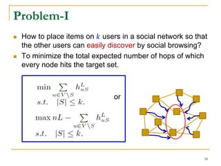
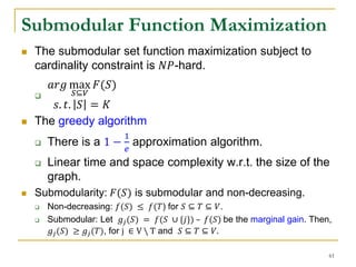
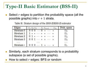
![ The submodular set function maximization subject to
cardinality constraint is 𝑁𝑃-hard.
𝑎𝑟𝑔 max
𝑆⊆𝑉
𝐹(𝑆)
𝑠. 𝑡. 𝑆 = 𝐾
Both Problem I and Problem II use a submodular set
function.
Problem-I: 𝐹1 S = nL − 𝑢∈𝑉𝑆 ℎ 𝑢𝑆
𝐿
Problem-II: 𝐹2(𝑆) = 𝑤∈𝑉 𝔼[𝑋 𝑤𝑆
𝐿
] = 𝑤∈𝑉 𝑝 𝑤𝑆
𝐿
Submodular Function Maximization
62](https://image.slidesharecdn.com/jeffreyxuyu-largegraphprocessing-160616082809/85/Jeffrey-xu-yu-large-graph-processing-62-320.jpg)
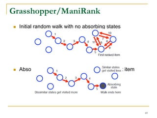
![Diversified Ranking [Li et al, TKDE’13]
Why diversified ranking?
Information requirements diversity
Query incomplete
PAKDD09-65](https://image.slidesharecdn.com/jeffreyxuyu-largegraphprocessing-160616082809/85/Jeffrey-xu-yu-large-graph-processing-65-320.jpg)


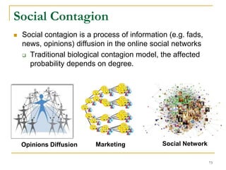
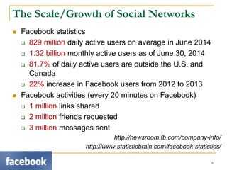
![Facebook Study [Ugander et al., PNAS’12]
Case study: The process of a user joins Facebook in
response to an invitation email from an existing
Facebook user.
Social contagion is not like biological contagion.
74](https://image.slidesharecdn.com/jeffreyxuyu-largegraphprocessing-160616082809/85/Jeffrey-xu-yu-large-graph-processing-74-320.jpg)

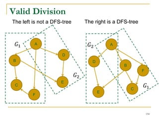
![A
B
D
C
I
E
F
G
H
A
B
C
G
F
Main Memory
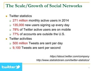
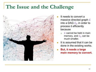
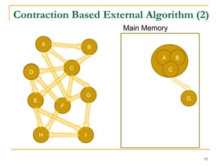
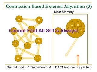
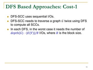
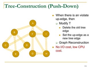
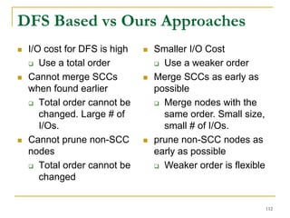
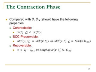
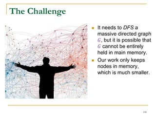
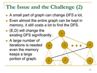
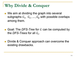
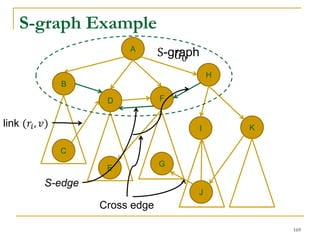
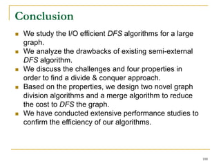
Contraction Based External Algorithm (1)
Load in a subgraph and merge SCCs
in it in main memory in every iteration
[Cosgaya-Lozano et al. SEA'09]
91](https://image.slidesharecdn.com/jeffreyxuyu-largegraphprocessing-160616082809/85/Jeffrey-xu-yu-large-graph-processing-91-320.jpg)
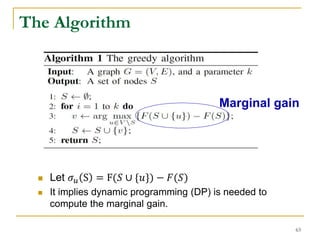
![2
8
3
4
7
5
1
9
6
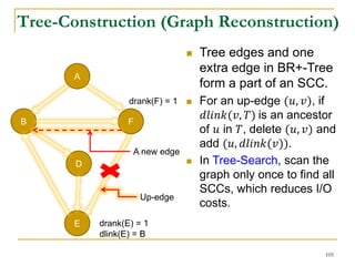
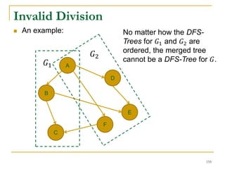
Tree-Edge
Forward-Cross-Edge
Backward-Edge
Forward-Edge
Backward-Cross-Edgedelete old tree edge
New tree edge
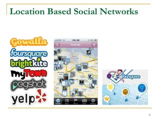
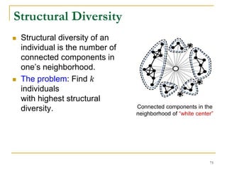
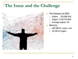
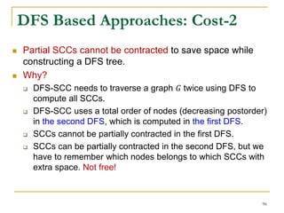
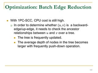
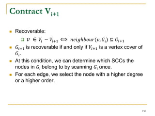
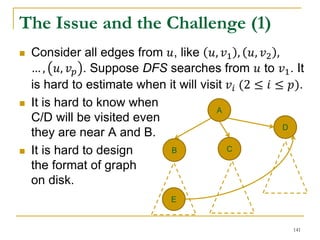
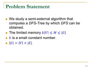
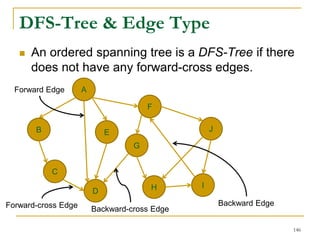
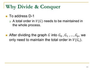
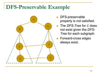
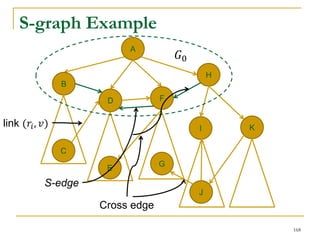
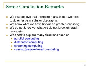
DFS Based Semi-External Algorithm
Find a DFS-tree without
forward-cross-edges
[Sibeyn et al. SPAA’02].
For a forward-cross-
edge (𝑢, 𝑣), delete tree
edge to 𝑣, and (𝑢, 𝑣) as
a new tree edge.
94](https://image.slidesharecdn.com/jeffreyxuyu-largegraphprocessing-160616082809/85/Jeffrey-xu-yu-large-graph-processing-94-320.jpg)
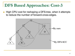
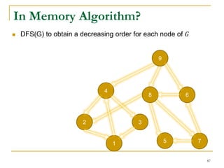
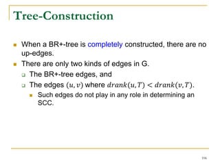
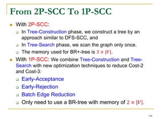
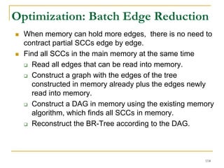
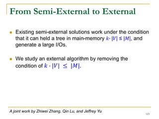
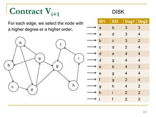
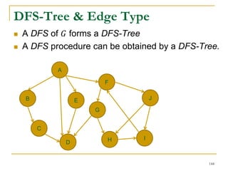
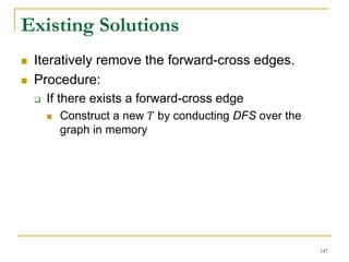
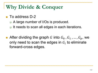
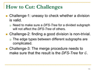
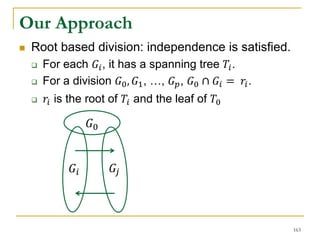
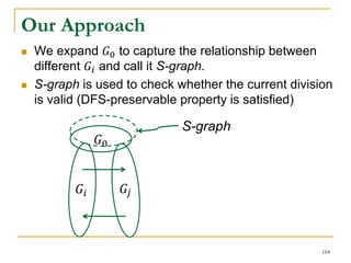
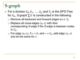
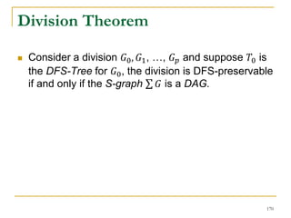
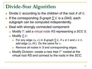
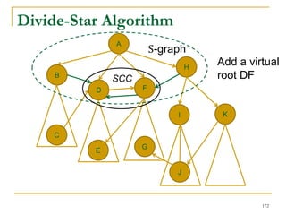
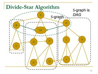
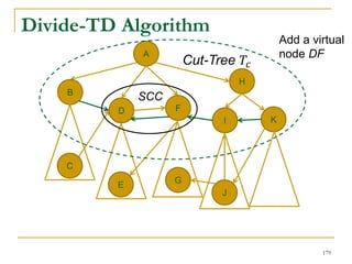
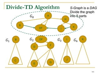
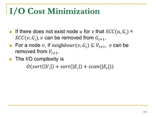
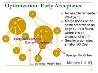
![Our New Approach [SIGMOD’13]
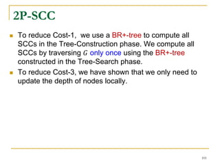
We propose a new two phase algorithm, 2P-SCC:
Tree-Construction and Tree-Search.
In Tree-Construction phase, we construct a tree-like
structure.
In Tree-Search phase, we scan the graph only once.
We further propose a new algorithm, 1P-SCC, to
combine Tree-Construction and Tree-Search with new
optimization techniques, using a tree.
Early-Acceptance
Early-Rejection
Batch Edge Reduction
A joint work by Zhiwei Zhang, Jeffrey Yu, Qin Lu, Lijun Chang, and Xuemin Lin
98](https://image.slidesharecdn.com/jeffreyxuyu-largegraphprocessing-160616082809/85/Jeffrey-xu-yu-large-graph-processing-98-320.jpg)
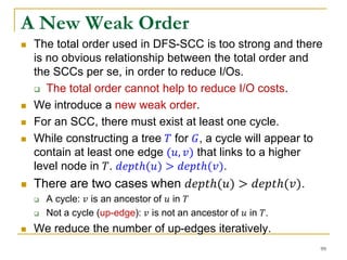
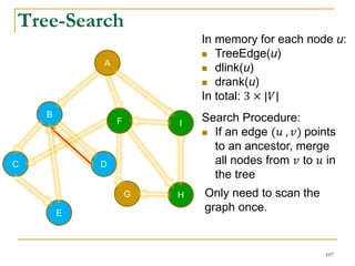
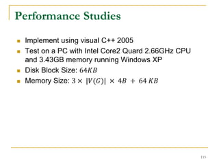

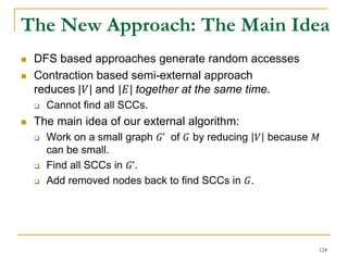
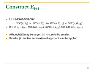
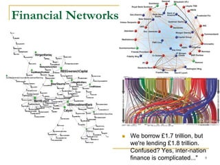
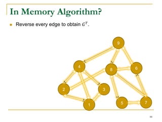
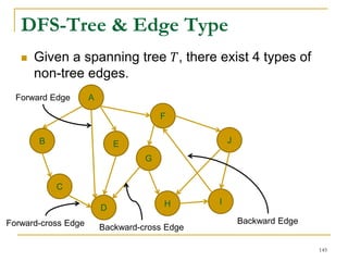
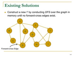
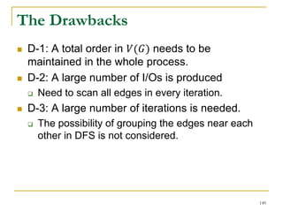
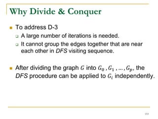
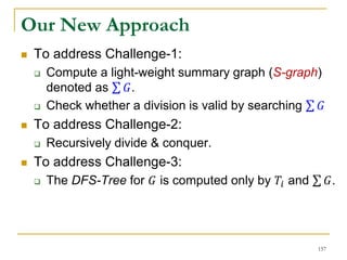
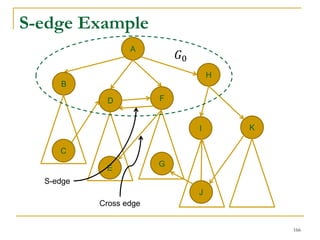
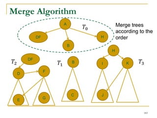
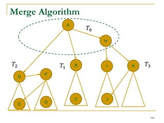
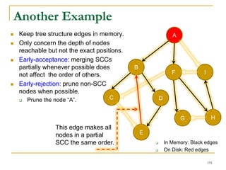
![DFS [SIGMOD’15]
Given a graph 𝐺(𝑉, 𝐸), depth-first search is to
search 𝐺 following the depth-first order.
A
B E
D
C
F
IH
J
G
A joint work by Zhiwei Zhang, Jeffrey Yu, Qin Lu, and Zechao Shang
139](https://image.slidesharecdn.com/jeffreyxuyu-largegraphprocessing-160616082809/85/Jeffrey-xu-yu-large-graph-processing-139-320.jpg)
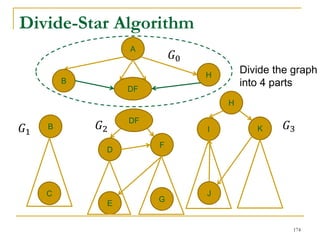


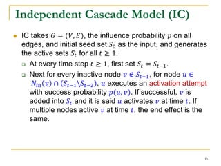
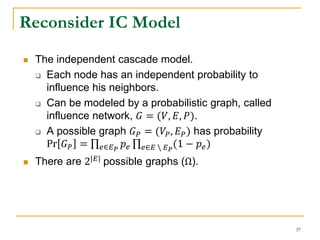
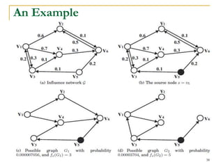
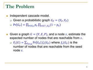
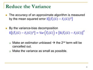
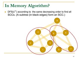
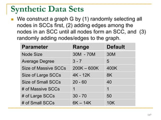
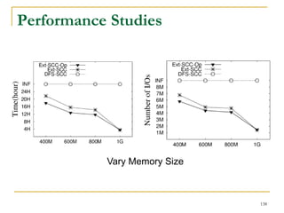
This document discusses influenceability estimation in social networks. It describes the independent cascade model of influence diffusion, where each node has an independent probability of influencing its neighbors. The problem is to estimate the expected number of nodes reachable from a given seed node. The document presents the naive Monte Carlo (NMC) approach, which samples possible graphs and averages the number of reachable nodes over the samples. While NMC provides an unbiased estimator, it has high variance. The document aims to reduce the variance to improve estimation accuracy.


![[CS570] Machine Learning Team Project (I know what items really are)](https://cdn.slidesharecdn.com/ss_thumbnails/finalprojectpresentation11-130618082905-phpapp02-thumbnail.jpg?width=640&height=640&fit=bounds)


![제 23회 보아즈(BOAZ) 빅데이터 컨퍼런스 - [MBOAX] : ABSA를 활용한 소비자 반응 분석 기반 운영 효율화 대시보드 설계](https://cdn.slidesharecdn.com/ss_thumbnails/3-1boaz23rdconferencemboax-260203102709-9d519923-thumbnail.jpg?width=640&height=640&fit=bounds)


![7.__Developing_a_Research_Proposal[1].pptx](https://cdn.slidesharecdn.com/ss_thumbnails/7-260131073037-df92dd7d-thumbnail.jpg?width=640&height=640&fit=bounds)

