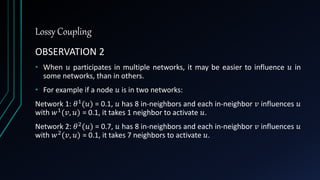
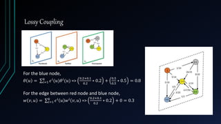
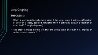
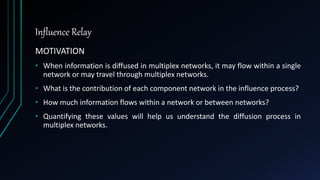
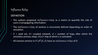
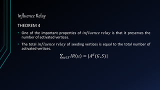
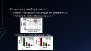
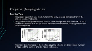
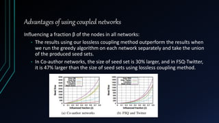
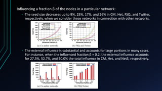
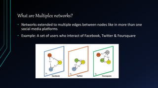
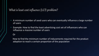
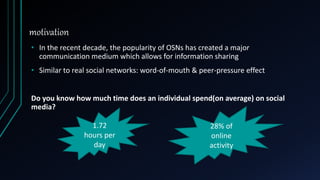
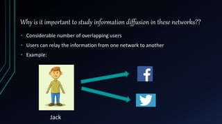
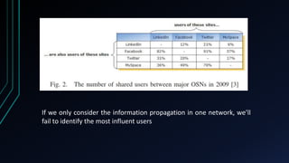
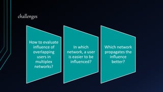
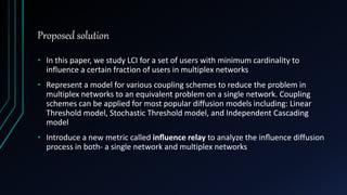
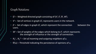
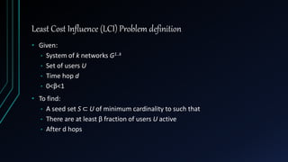
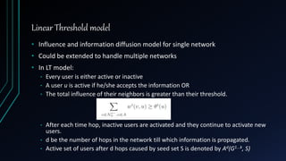
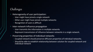
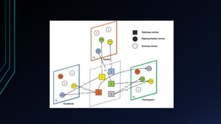
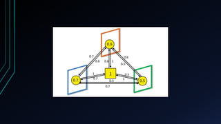
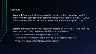
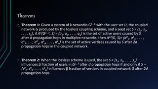
The document presents a model for analyzing the least cost influence (LCI) problem in multiplex social networks, focusing on how to optimize the selection of seed users to maximize overall influence with minimal cost. It discusses various coupling schemes to combine multiple networks without losing data and introduces new metrics for measuring influence propagation, such as influence relay. The findings suggest that the proposed methods can enhance information diffusion analysis within multiplex networks, allowing for more effective strategies in viral marketing and information dissemination.


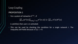
![Lossy Coupling
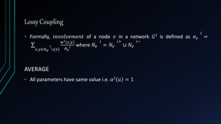
• 𝛼 𝑖 𝑢 can constitute for extra influence which may be required to activate 𝑢
• 𝛼 𝑖
𝑢 can be made proportional to 𝑣∈𝑁 𝑢
𝑖−
∩𝐴
𝑤 𝑖
(𝑣, 𝑢) − 𝜃 𝑖
(𝑢) . In this way,
when 𝑣∈𝑁 𝑢
𝑖−∩𝐴
𝑤 𝑖(𝑣, 𝑢) > 𝜃 𝑖 𝑢 we choose 𝛼 𝑖 𝑢 ≫ 𝛼 𝑗 𝑢 [∀𝑗 ≠ 𝑖].
• In real life, we don’t know in which network 𝑢 will be activated. Hence, we
have to use heuristics.](https://image.slidesharecdn.com/group11-151229011537/85/Least-Cost-Influence-in-Multiplex-Social-Networks-34-320.jpg)