JAMA - Guide to Statistics and Methods.pdf

Table of contents:
1. The Intention-to-Treat Principle
2. Noninferiority Trials
3. Sample Size Calculation for a Hypothesis Test
4. Interpretation of Clinical Trials That Stopped Early
5. Cluster Randomized Trials
6. Case-Control Studies
7. Decision Curve Analysis
8. Gatekeeping Strategies for Avoiding False-Positive Results in Clinical Trials With
Many Comparisons
9. Multiple Comparison Procedures
10. Pragmatic Trials
11. Equipoise in Research
12. The Propensity Score
13. Dose-Finding Trials
14. Odds Ratios—Current Best Practice and Use
15. Evaluating Discrimination of Risk Prediction Models
16. Time-to-Event Analysis
17. The Stepped-Wedge Clinical Trial
18. Mendelian Randomization
19. Bayesian Analysis: Using Prior Information to Interpret the Results of Clinical Trials
JAMA - Guide to Statistics and Methods

Copyright 2014 American Medical Association. All rights reserved.
The Intention-to-Treat Principle
How to Assess the True Effect of Choosing
a Medical Treatment
Michelle A. Detry, PhD; Roger J. Lewis, MD, PhD
The intention-to-treat (ITT) principle is a cornerstone in the in-
terpretationofrandomizedclinicaltrials(RCTs)conductedwiththe
goal of influencing the selection of medical therapy for well-
definedgroupsofpatients.TheITTprincipledefinesboththestudy
population included in the pri-
mary efficacy analysis and how
theoutcomesareanalyzed.Un-
der ITT, study participants are
analyzed as members of the treatment group to which they were
randomized regardless of their adherence to, or whether they re-
ceived,theintendedtreatment.1-3
Forexample,inatrialinwhichpa-
tientsarerandomizedtoreceiveeithertreatmentAortreatmentB,
a patient may be randomized to receive treatment A but errone-
ously receive treatment B, or never receive any treatment, or not
adhere to treatment A. In all of these situations, the patient would
beincludedingroupAwhencomparingtreatmentoutcomesusing
an ITT analysis. Eliminating study participants who were random-
ized but not treated or moving participants between treatment
groups according to the treatment they received would violate the
ITT principle.
In this issue of JAMA, Robertson et al conducted an RCT using
a factorial design to compare transfusion thresholds of 10 and 7
g/dL and administration of erythropoietin vs placebo in 895
patients with anemia and traumatic brain injury.4
The primary
outcome was the 6-month Glasgow Outcome Scale (GOS),
dichotomized so a good or moderate score indicated success. The
trial was conducted with high fidelity to the protocol so only a few
patients did not receive the intended treatment strategy. Two
patients randomized to the 7-g/dL study group were managed
according to the 10-g/dL threshold and an additional 2 patients
randomized to the 7-g/dL study group received one transfusion
not according to protocol. The authors implemented the ITT prin-
ciple and the outcomes for these 4 patients were included in the
7-g/dL group.
Use of the Method
Why Is ITT Analysis Used?
The effectiveness of a therapy is not simply determined by its
pure biological effect but is also influenced by the physician’s abil-
ity to administer, or the patient’s ability to adhere to, the intended
treatment. The true effect of selecting a treatment is a combina-
tion of biological effects, variations in compliance or adherence,
and other patient characteristics that influence efficacy. Only by
retaining all patients intended to receive a given treatment in
their original treatment group can researchers and clinicians
obtain an unbiased estimate of the effect of selecting one treat-
ment over another.
Treatment adherence often depends on many patient and cli-
nician factors that may not be anticipated or are impossible to
measure and that influence response to treatment. For example,
in the study by Robertson et al, some patients randomized to the
higher transfusion threshold may not have received the intended
therapeutic strategy due to adverse events associated with trans-
fusion, fluid overload, or unwillingness of clinicians to adhere to
the strategy for other reasons. These patients are likely to be fun-
damentally different from those who were actually treated using
the 10-g/dL strategy. The characteristics that differ between
patients who received the intended therapy and those who did
not could easily influence whether a successful GOS score is
achieved. If the ITT principle was not followed and patients were
removed from their randomized group and either ignored or
assigned to the other treatment group, the results of the analysis
would be biased and no longer represent the effect of choosing
one therapy over the other.
It is common to see alternative analyses proposed, eg, per-
protocol or modified intent-to-treat (MITT) analyses.5
A per-
protocol analysis includes only study participants who completed
the trial without any major deviations from the study protocol; this
usually requires that they successfully receive and complete their
assignedtreatment(s),completetheirstudyvisits,andprovidepri-
mary outcome data. The requirements to be included in the per-
protocol analysis vary from study to study. While the definition of
an MITT analysis also varies from study to study, the MITT ap-
proach deviates from the ITT approach by eliminating patients or
reassigningpatientstoastudygroupotherthanthegrouptowhich
theywererandomized.NeitheroftheseapproachessatisfiestheITT
principleandmayleadtoclinicallymisleadingresults.Ithasbeenob-
served that studies using MITT analysis are more likely to be posi-
tivethanthosefollowingastrictITTapproach.5
Acomparisonofre-
sultsfromITTandper-protocolorMITTanalysesmayprovidesome
indication of the potential effect of nonadherence on overall treat-
ment effectiveness.
Noninferiority trials, which are designed to demonstrate that
an experimental treatment is no worse than an established one,
require special considerations with regard to the ITT principle.6-8
Consider a noninferiority trial of 2 treatments— treatment A is a
biologically ineffective experimental therapy and treatment B is a
biologically effective standard therapy—with the goal to demon-
strate that treatment A is noninferior to B. Patients may be ran-
domized to receive treatment B, not adhere to the treatment,
and fail treatment due to their nonadherence. If this happens fre-
quently, treatment B will appear less efficacious. Thus, the inter-
vention in group A may incorrectly appear noninferior to the
intervention in group B, simply as a result of nonadherence rather
than because of similar biological efficacy. In this case, the ITT
Related article 36
Clinical Review & Education
JAMA Guide to Statistics and Methods
jama.com JAMA July 2, 2014 Volume 312, Number 1 85
Downloaded From: https://jamanetwork.com/ UFBA by Dimitri Gusmao-Flores on 10/10/2020

analysis is somewhat misleading because the noninferiority is a
result of poor adherence. In a noninferiority trial, both ITT and per-
protocol analyses should be conducted and reported. If the per-
protocol results are similar to the ITT results, the claim of noninferi-
ority is substantially strengthened.6-8
What Are the Limitations of ITT Analysis?
A characteristic of the ITT principle is that poor treatment adher-
ence may result in lower estimates of treatment efficacy and a loss
ofstudypower.However,theseestimatesareclinicallyrelevantbe-
causereal-worldeffectivenessislimitedbytheabilityofpatientsand
clinicians to adhere to a treatment.
Because all patients must be analyzed under the ITT principle,
it is essential that all patients be followed up and their primary out-
comesdetermined.Patientswhodiscontinuestudytreatmentsare
often more likely to be lost to follow-up. Following the ITT principle
will not eliminate bias associated with missing outcome data; steps
mustalwaysbetakentokeepmissingdatatoaminimumand,when
missingdataareunavoidable,touseminimallybiasingmethodsfor
adjusting for missing data (eg, multiple imputation).
Why Did the Authors Use ITT Analysis in This Particular Study?
Robertson et al4
used an ITT analysis because it allowed the effec-
tivenessoftheirtherapeuticstrategiestobeevaluatedwithoutbias
due to differences in adherence. Failure to follow the ITT principle
could have led to greater scrutiny of the trial results, especially if
adherence to the intended treatments had been poorer.
Caveats to Consider When Looking at Results
Based on ITT Analysis
Although the ITT principle is important for estimating the efficacy
oftreatments,itshouldnotbeappliedinthesamewayinassessing
thesafety(eg,medicationadverseeffects)ofinterventions.Forex-
ample,itwouldnotmakesensetoattributeanapparentadverseef-
fect to an intended treatment when, in fact, the patient was never
exposed to the experimental drug. For this reason, safety analyses
are generally conducted according to the treatment actually re-
ceived,eventhoughthismaynotaccuratelyestimate—andmaywell
overestimate—theburdenofadverseeffectslikelytobeseeninclini-
cal practice.
While determining the effect of choosing one treatment over
another, or over no treatment at all, is a key goal of trials conducted
lateintheprocessofdruganddevicedevelopment,thegoalsoftrials
conducted earlier in development are generally focused on nar-
rower questions such as biological efficacy and dose selection. In
thesecases,MITTandper-protocolanalysisstrategieshaveagreater
role in guiding the design and conduct of subsequent clinical trials.
For example, it would be unfortunate to falsely conclude, based on
the ITT analysis of a phase 2 clinical trial, that a novel pharmaceuti-
calagentisnoteffectivewhen,infact,thelackofefficacystemsfrom
too high a dose and patients’ inability to be adherent because of in-
tolerable adverse effects. In that case, a lower dose may yield clini-
callyimportantefficacyandatolerableadverseeffectprofile.Aper-
protocolanalysismaybehelpfulinsuchacase,allowingthedetection
of the beneficial effect in patients able to tolerate the new therapy.
ARTICLE INFORMATION
Author Affiliations: Berry Consultants LLC, Austin,
Texas (Detry, Lewis); Department of Emergency
Medicine, Harbor-UCLA Medical Center; Los
Angeles Biomedical Research Institute; and David
Geffen School of Medicine at UCLA, Torrance,
California (Lewis).
Corresponding Author: Roger J. Lewis, MD, PhD,
Department of Emergency Medicine, Harbor-UCLA
Medical Center, Bldg D9, 1000 W Carson St,
Torrance, CA 90509 (roger@emedharbor.edu).
Conflict of Interest Disclosures: The authors have
completed and submitted the ICMJE Form for
Disclosure of Potential Conflicts of Interest and
none were reported.
REFERENCES
1. Cook T, DeMets DL. Introduction to Statistical
Methods for Clinical Trials. Boca Raton, FL:
Chapman & Hall/CRC; Taylor & Francis Group;
2008:chp 11.
2. Schulz KF, Altman DG, Moher D; CONSORT
Group. CONSORT 2010 statement: updated
guidelines for reporting parallel group randomized
trials. Ann Intern Med. 2010;152(11):726-732.
3. Food and Drug Administration. Guidance for
industry e9 statistical principles for clinical trials.
http://www.fda.gov/downloads/Drugs
/GuidanceComplianceRegulatoryInformation
/Guidances/ucm073137.pdf. September 1998.
Accessed May 11, 2014.
4. Robertson CS, Hannay HJ, Yamal J-M, et al; and
the Epo Severe TBI Trial Investigators. Effect of
erythropoietin and transfusion threshold on
neurological recovery after traumatic brain injury:
a randomized clinical trial. JAMA. doi:10.1001/jama
.2014.6490.
5. Montedori A, Bonacini MI, Casazza G, et al.
Modified versus standard intention-to-treat
reporting: are there differences in methodological
quality, sponsorship, and findings in randomized
trials? a cross-sectional study. Trials. 2011;12:58.
6. Piaggio G, Elbourne DR, Pocock SJ, Evans SJ,
Altman DG; CONSORT Group. Reporting of
noninferiority and equivalence randomized trials:
extension of the CONSORT 2010 statement. JAMA.
2012;308(24):2594-2604.
7. Le Henanff A, Giraudeau B, Baron G, Ravaud P.
Quality of reporting of noninferiority and
equivalence randomized trials. JAMA. 2006;295
(10):1147-1151.
8. Mulla SM, Scott IA, Jackevicius CA, et al. How to
use a noninferiority trial: Users’ Guides to the
Medical Literature. JAMA. 2012;308:2605-2611.
Clinical Review & Education JAMA Guide to Statistics and Methods
86 JAMA July 2, 2014 Volume 312, Number 1 jama.com

Noninferiority Trials
Is a New Treatment Almost as Effective as Another?
Amy H. Kaji, MD, PhD; Roger J. Lewis, MD, PhD
Sometimes the goal of comparing a new treatment with a stan-
dard treatment is not to find an approach that is more effective but
tofindatherapythathasotheradvantages,suchaslowercost,fewer
adverse effects, or greater con-
venience with at least similar
efficacy to the standard treat-
ment. With other advantages, a
treatment that is almost as effective as a standard treatment might
bepreferredinpracticeorforsomepatients.Thepurposeofanon-
inferiority trial is to rigorously evaluate a new treatment against an
accepted and effective treatment with the goal of demonstrating
that it is at least almost as good (ie, not inferior).
In this issue of JAMA, Salminen et al describe the results of a
multicenter noninferiority trial of 530 adults with computed
tomography–confirmed acute appendicitis who were randomized
either to early appendectomy (the standard treatment) or to anti-
biotic therapy alone (a potentially less burdensome experimental
treatment).1
Use of the Method
Why Are Noninferiority Trials Conducted?
Inatraditionalclinicaltrial,anewtreatmentiscomparedwithastan-
dard treatment or placebo with the goal of demonstrating that the
new treatment has greater efficacy. The null hypothesis for such a
trial is that the 2 treatments have the same effect. Rejection of this
hypothesis, implying that the effects are different, is signaled by a
statistically significant P value or, alternatively, by a 2-tailed confi-
dence interval that excludes no effect. While the new treatment
could be either superior or inferior, the typical trial aims to demon-
strate superiority of the new treatment and is known as a superior-
ity trial. Since a superiority trial is capable of identifying both harm-
ful and beneficial effects of a new therapy vs a control (ie, a current
therapy), a 2-tailed 95% CI can be used to indicate the upper and
lower limits of the difference in treatment effect that are consis-
tent with the observed data. The null hypothesis is rejected, indi-
cating that the new therapy differs from the control, if the confi-
dence interval does not include the result that indicates absence of
effect (eg, a risk ratio of 1 or a risk difference of 0).2
This is equiva-
lent to a statistically significant P value.
Although superiority or inferiority of a new treatment can be
demonstrated by a superiority trial, it would generally be incorrect
to conclude that the absence of a significant difference in a superi-
ority trial demonstrates that the therapies have similar effects; ab-
sence of evidence of a difference is not reliable evidence that there
is no difference. An active-controlled noninferiority trial is needed
to determine whether a new intervention, which offers other ad-
vantagessuchasdecreasedtoxicityorcost,doesnothavelesseref-
ficacy than an established treatment.3-6
Noninferiority trials use
known effective treatments as controls because there is little to be
gainedbydemonstratingthatanewtherapyisnotinferiortoasham
or placebo treatment.
Theobjectiveofanoninferioritytrialistodemonstratethatthe
intervention being evaluated achieves the efficacy of the estab-
lishedtherapywithinapredeterminedacceptablenoninferioritymar-
gin (Figure). The magnitude of this margin depends on what would
be a clinically important difference, the expected event rates, and,
possibly, regulatory requirements. Other determinants of the non-
inferiority margin include the known effect of the standard treat-
ment vs placebo; the severity of the disease; toxicity, inconve-
nience,orcostofthestandardtreatment;andtheprimaryendpoint.
Asmallernoninferioritymarginislikelyappropriateifthediseaseun-
der investigation is severe or if the primary end point is death.3-6
The sample size required to reliably demonstrate noninferior-
itydependsonboththechoiceofthenoninferioritymarginandthe
assumedtruerelativeeffectsofthecomparedtreatments.3-6
Anac-
tive-controllednoninferioritytrialoftenrequiresalargersamplesize
than a superiority trial because the noninferiority margins used in
noninferiority studies are generally smaller than the differences
sought in superiority trials. Just as important is the assumed effect
of the experimental treatment relative to the active-control treat-
ment.Theassumedeffectmaybethattheexperimentaltreatment
is worse than the control but by a smaller amount than the nonin-
feriority margin, that the 2 treatments are equivalent, or even that
Related article page 2340
Figure. Two Different Possible Results of a Noninferiority Trial,
Summarized by 1-Tailed Confidence Intervals for the Relative Efficacy of
the New and Active-Control Treatments
Active
Control
Better
New
Treatment
Better
Noninferiority
margin
Noninferiority not demonstrated
Noninferiority demonstrated
– +
∞
∞
Difference in Efficacy
(New Treatment Minus Active Control)
0
In the top example, the lower limit of the confidence interval lies to the left of the
noninferiority margin, demonstrating that the results are consistent with greater
inferiority (worse efficacy) than allowed by the noninferiority margin. Thus, the
new treatment may be inferior and noninferiority is not demonstrated. In the
lower example, the lower limit of the confidence interval lies to the right of the
noninferiority margin, demonstrating noninferiority of the new treatment relative
to the active-control treatment. The overall result of the trial is defined by the
lower limit of the 1-sided confidence interval rather than by the point estimate for
the treatment effect, so point estimates are not shown.
jama.com (Reprinted) JAMA June 16, 2015 Volume 313, Number 23 2371

the experimental treatment is more effective. These 3 options will
resultinlarger,intermediate,andsmallerrequiredsamplesizes,re-
spectively, to achieve the same trial power—the chance of demon-
strating noninferiority—because they assume progressively better
efficacy of the experimental treatment.
Because a noninferiority trial only aims to demonstrate nonin-
feriority and does not aim to distinguish noninferiority from supe-
riority, it is analyzed using a 1-sided confidence interval (Figure) or
hypothesistest.Typically,a1-sided95%or97.5%CI(−Lto!;nega-
tive values represent inferiority of the experimental treatment) is
constructed for the difference between the 2 treatments, and the
lower limit, −L, is compared with the noninferiority margin. Nonin-
feriority is demonstrated if the lower confidence limit lies above or
to the right of the noninferiority margin.3-6
What Are the Limitations of Noninferiority Trials?
A negative noninferiority trial does not in general demonstrate in-
feriority of the experimental treatment, just as a negative superior-
ity trial does not demonstrate equivalence of 2 treatments.
A noninferiority trial is similar to an equivalence trial in that the
objective of both is to demonstrate that the intervention matches
the action of the established therapy within a prespecified margin.
However, the objective of a noninferiority trial is only to demon-
stratethattheexperimentaltreatmentisnotsubstantiallyworsethan
the standard treatment, whereas that of an equivalence trial is to
demonstratethattheexperimentaltreatmentisneitherworsethan
nor better than the standard treatment.3
Why Was a Noninferiority Trial Conducted in This Case?
Ever since McBurney demonstrated reduced morbidity from pelvic
infectionswithappendectomy,thestandardtreatmentforacuteap-
pendicitis has been surgery, which requires general anesthesia, in-
cursincreasedcost,andisassociatedwithpostoperativecomplica-
tions,suchaswoundinfectionsandadhesions.Thus,alessinvasive
approach with similar efficacy might be preferred by many pa-
tients and physicians. Three randomized trials summarized in a re-
cent Cochrane analysis demonstrated equipoise as to whether ap-
pendicitis can successfully be treated with antibiotics alone rather
than surgery.7
Because appendectomy is viewed as the standard
treatment, it was considered the active control with which the less
invasive experimental antibiotic treatment was to be compared.
Todesigntheclinicaltrial,Salminenetalassumedasurgicaltreat-
ment success rate of 99% and prespecified a noninferiority margin
of −24% based on clinical considerations. This is equivalent to say-
ingthatiftherateoftreatmentsuccesswithantibioticsalonecould
be shown to be no worse than 24% worse than the rate with sur-
gery, then the antibiotic-only strategy would be clinically noninfe-
rior. As this study demonstrates, the selection of the noninferiority
margin is often subjective rather than based on specific criteria.
How Should the Results Be Interpreted?
The results demonstrated that all but 1 of 273 patients randomized
to the surgery group underwent successful appendectomy, result-
ing in a treatment efficacy of 99.6%. In the antibiotic treatment
group,186of256patientsavailableforfollow-uphadtreatmentsuc-
cesses, for a success rate of 72.7%; 70 of the 256 patients under-
wentsurgicalinterventionwithin1yearofinitialpresentation.Thus,
the point estimate for the difference in success rate with the anti-
biotic-only strategy was −27.0% and the associated 1-tailed 95% CI
would range from −31.6% to infinity. Because that interval includes
efficacy values worse than the noninferiority margin of −24%, non-
inferiority cannot be demonstrated.
Caveats to Consider When Looking at a Noninferiority Trial
Noninferiority active-controlled trials often require a larger sample
sizethanplacebo-controlledtrials,inpartbecausethechosennon-
inferioritymarginsareoftensmall.Therequiredsamplesizeforanon-
inferioritytrialishighlydependentonthenoninferioritymarginand
theassumedeffectofthenewtreatment;thisassumedeffectmust
be clearly stated and realistic.
The primary analysis for a superiority trial should be based on
the intention-to-treat (ITT) principle because it is generally conser-
vative in the setting of imperfect adherence to treatment. How-
ever, analyzing a noninferiority trial by ITT could make an inferior
treatment appear to be noninferior if poor patient adherence re-
sultedinbothtreatmentsbeingsimilarlyineffective.Thus,whenana-
lyzinganoninferioritytrial,bothITTandper-protocolanalysesshould
be conducted. The results are most meaningful when both ap-
proaches demonstrate noninferiority.
Anoninferioritytrialdoesnotdistinguishbetweenanewtreat-
ment that is noninferior and one that is truly superior and cannot
demonstrate equivalence.
ARTICLE INFORMATION
Author Affiliations: Department of Emergency
Medicine, Harbor-UCLA Medical Center, Torrance,
California (Kaji, Lewis); David Geffen School
of Medicine at UCLA, Torrance, California
(Kaji, Lewis); Los Angeles Biomedical Research
Institute, Los Angeles, California (Kaji, Lewis);
Berry Consultants, LLC (Lewis).
Medical Center, 1000 W Carson St, Box 21,
Section Editors: Roger J. Lewis, MD, PhD,
Medical Center and David Geffen School of
Medicine at UCLA; and Edward H. Livingston, MD,
Deputy Editor, JAMA.
none were reported.
REFERENCES
1. Salminen P, Paajanen H, Rautio T, et al. Antibiotic
therapy vs appendectomy for treatment of
uncomplicated acute appendicitis: the APPAC
randomized clinical trial. JAMA. doi: 10.1001/jama
.2015.6154.
2. Young KD, Lewis RJ. What is confidence? I: the
use and interpretation of confidence intervals. Ann
Emerg Med. 1997;30(3):307-310.
3. Kaji AH, Lewis RJ. Are we looking for superiority,
equivalence, or noninferiority? Ann Emerg Med.
2010;55(5):408-411.
4. Mulla SM, Scott IA, Jackevicius CA, et al. How to
use a non-inferiority trial: Users’ Guides to the
Medical Literature. JAMA. 2012;308:2605-2611.
5. Tamayo-Sarver JH, Albert JM, Tamayo-Sarver M,
Cydulka RK. Advanced statistics: how to determine
whether your intervention is different, at least as
effective as, or equivalent. Acad Emerg Med. 2005;
12(6):536-542.
6. Piaggio G, Elbourne DR, Altman DG, Pocock SJ,
Evans SJW; CONSORT Group. Reporting of
noninferiority and equivalence randomized trials:
an extension of the CONSORT statement. JAMA.
2006;295(10):1152-1160.
7. Wilms IM, de Hoog DE, de Visser DC, Janzing
HM. Appendectomy vs antibiotic treatment for
acute appendicitis. Cochrane Database Syst Rev.
2011;(11):CD008359.
2372 JAMA June 16, 2015 Volume 313, Number 23 (Reprinted) jama.com

Sample Size Calculation for a Hypothesis Test
Lynne Stokes, PhD
In this issue of JAMA, Koegelenberg et al1
report the results of a
randomized clinical trial (RCT) that investigated whether treat-
ment with a nicotine patch in addition to varenicline produced
higher rates of smoking absti-
nence than varenicline alone.
The primary results were posi-
tive; that is, patients receiving
the combination therapy were more likely to achieve continuous
abstinence at 12 weeks than patients receiving varenicline alone.
The absolute difference in the abstinence rate was estimated to
be approximately 14%, which was statistically significant at level
α = .05.
These findings differed from the results reported in 2 previous
studies2,3
of the same question, which detected no difference in
treatments. What explains this difference? One explanation of-
fered by the authors is that the previous studies “…may have been
inadequatelypowered,”whichmeansthesamplesizeinthosestud-
ies may have been too small to identify a difference between the
treatments tested.
Use of the Method
Why Is Power Analysis Used?
The sample size in a research investigation should be large enough
thatdifferencesoccurringbychancearerarebutshouldnotbelarger
than necessary, to avoid waste of resources and to prevent expo-
sure of research participants to risk associated with the interven-
tions. With any study, but especially if the study sample size is very
small, any difference in observed rates can happen by chance and
thus cannot be considered statistically significant.
In developing the methods for a study, investigators conduct a
power analysis to calculate sample size. The power of a hypothesis
test is the probability of obtaining a statistically significant result
when there is a true difference in treatments. For example, sup-
pose, as Koegelenberg et al1
did, that the smoking abstinence rate
were45%forvareniclinealoneand14%larger,or59%,forthecom-
bination regimen. Power is the probability that, under these condi-
tions, the trial would detect a difference in rates large enough to be
statisticallysignificantatacertainlevelα(ie,αistheprobabilityofa
type I error, which occurs by rejecting a null hypothesis that is ac-
tually true).
Power can also be thought of as the probability of the comple-
ment of a type II error. If we accept a 20% type II error for a differ-
enceinratesofsized,wearesayingthatthereisa20%chancethat
we do not detect the difference between groups when the differ-
enceintheirratesisd.Thecomplementofthis,0.8 = 1 − 0.2,orthe
statistical power, means that when a difference of d exists, there is
an 80% chance that our statistical test will detect it.
The Figure illustrates the relationship between sample size
and power for the test described. The orange line shows the
power for the parameter settings above (baseline rate of 45% and
minimum detectable difference, or MDD, of 14%), when signifi-
cance level α is set to .05. For this scenario, the authors’ target
sample size of 398 (199 in each group) will produce a power of
80%. All these values (45%, 14%, .05, 80%) must be selected at
the planning stage of the study to carry out this calculation. The
significance level and power are “rule-of-thumb” choices and are
typically not based on the specifics of the study. If the researcher
wants to reduce the probability of making a type I error (α = .05)
or to increase the probability of detecting the specified difference
(power = 80%), then these values can be changed. Either change
will require a larger sample size.
Selecting the baseline rate and MDD requires the expertise of
the researcher. The baseline rate is typically available from the lit-
erature, because this rate is often based on a therapy that has
been studied. The MDD choice is more subjective. It should be a
clinically meaningful rate difference, or a scientifically important
rate difference, or both, that is also feasible to detect. For
example, if the combination therapy of varenicline and nicotine
patch increased abstinence by 0.1%, this difference would not be
of practical benefit, would require an extremely large sample size,
and would thus be too small a setting for the MDD. If the MDD
were specified as 50%, the new therapy would have to be 95%
effective (45% + 50%) before there would be a high chance of
detecting any difference, so would be too large for the MDD. The
authors based their choice of MDD = 14% on a compromise
between their judgment of a clinically important difference, 12%,
and the scientifically meaningful value of 16%. The 16% rate was
the observed difference in a study that compared varenicline
alone and together with nicotine gum.4
Thus, the ability to con-
Figure. Power for Detecting Difference and Sample Size
MDD=12%
MDD=14%
100
80
60
40
20
0
0 350
300
Power,
%
Sample Size for Each Group, No.
50 100 150 250
200
For a baseline rate of 45% and a minimum detectable difference (MDD) of 14%,
the target sample size of 398 (199 in each group) will produce a power of 80%
when α is set to .05. When the MDD is 12%, the resulting sample size is 542
(2 × 271) to achieve a power of 80%.
180 JAMA July 9, 2014 Volume 312, Number 2 jama.com

firm a difference that is slightly smaller for a related treatment
was considered scientifically important.
What Are the Limitations of Power Analysis?
Calculationofsamplesizerequirespredictionsofbaselineratesand
MDD, which may not be readily available, before the study begins.
The sample size is especially sensitive to the MDD. This is illus-
trated by the blue line in the Figure, which shows the sample size
neededinthisstudyiftheMDDweresetto12%.Theresultingsample
size is 542 (2 × 271) to achieve a power of 80%.
This method of conducting a power analysis might also pro-
duce the incorrect sample size if the data analysis conducted dif-
fers from that planned. For example, if abstinence were affected
by other covariates, such as age, and the groups were unbalanced
on this variable, other analyses might be used, such as logistic
regression models accounting for covariate differences. The
sample size that would be appropriate for one analysis may be
too large or small to achieve the same power with another ana-
lytic procedure.
Why Did the Authors Use Power Analysis in This Particular Study?
The number of research participants available for any study is lim-
ited by resources. However, the authors were aware that previous
studies comparing these treatments had found no significant dif-
ference in abstinence rates. This can occur even if a difference
exists if the sample size is too small. The authors wanted to
ensure that their sample size was adequate to detect even a small
but clinically important difference, so they carefully evaluated
sample size.
How Should This Method’s Findings Be Interpreted
in This Particular Study?
A power analysis can help with the interpretation of study findings
when statistically significant effects are not found. However, be-
cause the findings in the study by Koegelenberg et al1
were statis-
ticallysignificant,interpretationofalackofsignificancewasunnec-
essary.Ifnostatisticallysignificantdifferenceinabstinencerateshad
beenfound,theauthorscouldhavenotedthat,“Thestudywassuf-
ficientlypoweredtohaveahighchanceofdetectingadifferenceof
14% in abstinence rates. Thus, any undetected difference is likely
to be of little clinical benefit.”
Caveats to Consider When Looking at Results Based
on Power Analysis
Sample size calculation based on any power analysis requires input
from the researcher prior to the study. Some of these are assump-
tions and predictions of fact (such as the baseline rate), which may
be incorrect. Others reflect the clinical judgment of the researcher
(eg, MDD), with which the reader may disagree. If a statistically sig-
nificanteffectisnotfound,thereadershouldassesswhethereither
of these are concerns.
Thereadershouldalsonotinterpretalackofsignificanceforan
outcomeotherthantheoneonwhichthepoweranalysiswasbased
asconfirmationthatnodifferenceexists,becausetheanalysisisspe-
cific to the parameter settings. For example, no significant differ-
ence was found in this study for most adverse events rates, al-
though the power analysis does not apply to these rates. Thus, the
sample size may not be adequate to interpret that finding to con-
firm that no meaningful difference in these outcomes exists.
ARTICLE INFORMATION
Author Affiliation: Department of Statistical
Science, Southern Methodist University, Dallas,
Texas.
Corresponding Author: Lynne Stokes, PhD,
Department of Statistical Science, Southern
Methodist University, PO Box 750100, Dallas, TX
75275 (slstokes@smu.edu).
Conflict of Interest Disclosures: The author has
none were reported.
REFERENCES
1. Koegelenberg CFN, Noor F, Bateman ED, et al.
Efficacy of varenicline combined with nicotine
replacement therapy vs varenicline alone for
smoking cessation: a randomized clinical trial. JAMA.
doi:10.1001/jama.2014.7195.
2. Hajek P, Smith KM, Dhanji AR, McRobbie H. Is a
combination of varenicline and nicotine patch more
effective in helping smokers quit than varenicline
alone? a randomised controlled trial. BMC Med.
2013;11:140.
3. Ebbert JO, Burke MV, Hays JT, Hurt RD.
Combination treatment with varenicline and
nicotine replacement therapy. Nicotine Tob Res.
2009;11(5):572-576.
4. Besada NA, Guerrero AC, Fernandez MI, Ulibarri
MM, Jiménez-Ruiz CA. Clinical experience from a
smokers clinic combining varenicline and nicotine
gum. Eur Respir J. 2010;36(suppl 54):462s.
JAMA Guide to Statistics and Methods Clinical Review & Education
jama.com JAMA July 9, 2014 Volume 312, Number 2 181

Interpretation of Clinical Trials That Stopped Early
Kert Viele, PhD; Anna McGlothlin, PhD; Kristine Broglio, MS
Clinical trials require significantresources to complete in terms of
patients, investigators, and time and should be carefully designed
and conducted so that they use the minimum amount of resources
necessary to answer the motivating clinical question. The size of a
clinical trial is typically based on the minimum number of patients
required to have high probability of detecting the anticipated treat-
ment effect. However, it is possible that strong evidence could
emerge earlier in the trial either in favor of or against the benefit of
the novel treatment. If early trial results are compelling, stopping
the trial before the maximum planned sample size is reached pre-
sents ethical advantages for patients inside and outside the trial
and can save resources that can be redirected to other clinical
questions. This advantage must be balanced against the potential
for overestimation of the treatment effect and other limitations of
smaller trials (eg, limited safety data, less information about treat-
ment effects in subgroups).
Manymethodshavebeenproposedtoallowformalincorpora-
tion of early stopping into a clinical trial.1,2
All of these methods al-
low a trial to stop at a prespecified interim analysis while maintain-
inggoodstatisticalproperties.Datamonitoringcommitteesorother
similargoverningbodiesmayalsomonitortheprogressofatrialand
recommend stopping the trial early in the absence of a prespeci-
fiedformalrule.Anoverwhelminglypositivetreatmenteffectmight
lead to a recommendation for unplanned early stopping but, more
commonly,unplannedearlystoppingresultsfromconcernsforpar-
ticipant safety, lack of observed benefit, or concerns about the fea-
sibility of continuing the trial due to slow patient accrual or new ex-
ternal information. Trials stopped for success in an ad hoc manner
arechallengingtointerpretrigorously.Inthisarticle,wefocusonearly
stopping for success or futility based on formal, prespecified stop-
ping rules.
In the December 15, 2015, issue of JAMA, Stupp et al3
reported
the results of a trial assessing electric tumor-treating fields plus te-
mozolomide vs temozolomide alone in patients with glioblastoma.
The trial design included a preplanned interim analysis defined ac-
cordingtoanearlystoppingprocedure.Thetrialwasstoppedforsuc-
cess at the interim analysis, reporting a hazard ratio of 0.62 for the
primary end point of progression-free survival.
Use of the Method
Why Is Early Stopping Used?
When 2 treatments are compared in a randomized clinical trial, the
treatment effects observed both during the trial and when the trial
endsaresubjecttorandomhighsandlowsthatdepartfromthetrue
treatment effect. Sample sizes for trials are selected to reliably de-
tect an anticipated treatment effect even if a modest, random low
observed treatment effect occurs at the final analysis. If such a ran-
dom low value does not occur or the true treatment effect is larger
than anticipated, the extra study participants required to provide
this protection against a false-negative result may not be neces-
sary. During the course of a trial, strong evidence may accumulate
that the experimental treatment offers a benefit. This may be from
a large observed treatment effect emerging early in a trial or from
the anticipated treatment effect being observed as early as two-
thirds of the way through a trial.
Conversely, evidence could accumulate early in a trial that the
experimental treatment performs no better than the control. In a
trial with no provision for early stopping, patients would continue
to be exposed to the potential harms of the experimental therapy
with no hope of benefit. Interim analyses to stop trials early for fu-
tilitymayavoidthisrisk.Trialsmayalsostopearlyforfutilityifthere
is a limited likelihood of eventual success.4
What Are the Limitations of Early Stopping?
One key statistical issue with early stopping, particularly early stop-
ping for success, is accounting for multiple “looks” at the data. Accu-
mulating data, particularly early in the trial with a smaller number of
observations, is likely to exhibit larger random highs and lows of val-
ues for the treatment effects. The more frequently the data are ana-
lyzedastheyaccumulate,thegreaterthechanceofobservingoneof
these fluctuations. Rules allowing early stopping therefore require a
higherlevelofevidence,suchasalowerPvalue,ateachinterimanaly-
sis than would be required at the end of a trial with no potential for
early stopping. Taken together, the multiple looks at the data, each
requiring a higher bar for success, lead to the same overall chance of
falsely declaring success (type I error) as a trial with the usual crite-
rion for success (eg, a P<.05) and no potential for early stopping.
Early stopping for futility requires no such adjustment. There
are no added opportunities to declare a success; thus, no statistical
adjustment to the success threshold is required. However, futility
stopping may reduce the power of the trial by stopping trials based
onarandomlowvalueforthetreatmenteffectthatcouldhavegone
on to be successful. This reduction in power is usually quite small.
Success thresholds are typically chosen to be more conserva-
tive for interim analyses than for the final analysis should the trial
continue to completion. The O’Brien-Fleming method, for ex-
ample, requires very small P values to declare success early in the
trial and then maintains a final P value very close to the traditional
.05levelatthefinalanalysis.1
Usingthismethod,veryfewtrialscould
besuccessfulattheinterimanalysesthatwouldnothavebeensuc-
cessfulatthefinalanalysis.Thus,thereisaminimal“penalty”forthe
interim analyses. The more conservative the early stopping crite-
ria, the more assurance there is that an early stop for success is not
a false-positive result.
While methods such as O’Brien-Fleming protect against falsely
declaring an ineffective drug successful, the accuracy of estimates
of the treatment effect in trials that have stopped early for success
remains a concern.5
When considering the true effect of a treat-
ment, bias is introduced when considering only trials that have ob-
servedalargeenoughtreatmenteffecttomeetthecriticalvaluefor
1646 JAMA April 19, 2016 Volume 315, Number 15 (Reprinted) jama.com

success. By definition, successful trials have larger treatment ef-
fectsthanunsuccessfultrials;thus,successfultrialsincludemoreran-
dom highs than random lows. As such, small trials that end in suc-
cess, either at the end or early, are prone to overestimating the
treatmenteffect.Thelargertheobservedtreatmenteffect,themore
likely it is an extreme random high, and the greater the chance for
overestimation. If the trial were continued, with the enrollment of
additionalpatients,itislikelythattherewouldbeareductionofthe
observed treatment effect. In other words, trials with very impres-
sive early results are likely to become less impressive after observ-
ing more data, and this should be taken into account when moni-
toring and interpreting such trials. Extreme attenuation, such as a
complete disappearance of the observed treatment benefit, how-
ever, is less likely.
Why Did the Authors Use Early Stopping in This Study?
Glioblastoma is an aggressive cancer with few treatment options.
InthereportbyStuppetal,3
enrollmentwaslargelycompleteatthe
time of the interim analysis. However, the interim analysis allowed
the possibility that a beneficial result could be disseminated many
months(potentiallyyears)earlierinadvanceofthefullymaturedata.
How Should Early Stopping Be Interpreted in This Particular Study?
The primary analysis in this study found a hazard ratio of 0.62
(P = .001) based on 18 months of follow-up from the first 315 pa-
tientsenrolled.Thisisstrongevidenceofatreatmentbenefitfortu-
mor-treating fields plus temozolomide in this population. How-
ever,careshouldbetakenwheninterpretingtheestimatedbenefit
corresponding to a hazard ratio of 0.62. Given the potential for an
overestimatedtreatmenteffect,combinedwiththegeneralintrac-
tabilityoftreatingglioblastoma,thereisgoodreasontosuspectthat
the actual benefit of tumor-treating fields, while present, might be
smaller than that observed in the study. A robustness analysis (ie, a
supplementary or supporting analysis conducted to see how con-
sistent the results are if different approaches were taken in con-
ductingtheanalysis),basedonthethen-availabledatafromallpar-
ticipants, illustrates this pattern. That analysis resulted in a hazard
ratio of 0.69 (95% CI, 0.55-0.86), also with a P<.001. The result re-
mained statistically significant, but the magnitude of the treat-
ment effect was smaller.
Caveats to Consider When Looking at a Trial
That Stopped Early
Itisimportanttoconsidertrialdesign,qualityoftrialconduct,safety
and secondary end points, and other supplementary data when in-
terpretingtheresultsofanyclinicaltrial.Fortrialsthatstopearlyfor
success, the statistical superiority of an experimental treatment is
straightforward when the early stopping was preplanned and it is
reasonable to preserve patient resources and time once the pri-
mary objective of a trial has been addressed. Early stopping proce-
dures protect against a false conclusion of superiority. However, if
theresultseemsimplausiblygood,thereisahighlikelihoodthatthe
trueeffectissmallerthantheobservedeffect.Inthatlight,theben-
efits of early stopping, to patients both in and out of the trial, must
beweighedagainsthowmuchpotentialadditionalknowledgewould
be gained if the trial were continued.
ARTICLE INFORMATION
Author Affiliations: Berry Consultants LLC,
Austin, Texas.
Corresponding Author: Kert Viele, PhD,
Berry Consultants LLC, 4301 Westbank Dr,
Bldg B, Ste 140, Austin, TX 78746
(kert@berryconsultants.com).
Conflict of Interest Disclosures: All authors have
none were reported.
REFERENCES
1. Jennison C, Turnbull BW. Group Sequential
Methods With Applications to Clinical Trials.
Boca Raton, FL: Chapman & Hall; 2000.
2. Broglio KR, Connor JT, Berry SM. Not too big,
not too small: a Goldilocks approach to sample size
selection. J Biopharm Stat. 2014;24(3):685-705.
3. Stupp R, Taillibert S, Kanner AA, et al.
Maintenance therapy with tumor-treating fields
plus temozolomide vs temozolomide alone for
glioblastoma: a randomized clinical trial. JAMA.
2015;314(23):2535-2543.
4. Saville BR, Connor JT, Ayers GD, Alvarez J.
The utility of Bayesian predictive probabilities for
interim monitoring of clinical trials. Clin Trials. 2014;
11(4):485-493.
5. Zhang JJ, Blumenthal GM, He K, Tang S, Cortazar
P, Sridhara R. Overestimation of the effect size in
group sequential trials. Clin Cancer Res. 2012;18(18):
4872-4876.
jama.com (Reprinted) JAMA April 19, 2016 Volume 315, Number 15 1647

Cluster Randomized Trials
Evaluating Treatments Applied to Groups
William J. Meurer, MD, MS; Roger J. Lewis, MD, PhD
Sometimes a new treatment is best introduced to an entire group
of patients rather than to individual patients. Examples include
when the new approach requires procedures be followed by mul-
tiple members of a health care team or when the new technique is
applied to the environment of care (eg, a method for cleaning a
hospital room before it is known which patient will be assigned the
room). This avoids confusion that could occur if all caregivers had
to keep track of which patients were being treated the old way and
which were being treated the new way.
One approach to evaluate the efficacy of such treatments—
treatments for which the application typically involves changes at
the level of the health care practice, hospital unit, or even health
care system—is to conduct a cluster randomized trial. In a cluster
randomized trial, study participants are randomized in groups or
clusters so that all members within a single group are assigned to
either the experimental intervention or the control.1,2
This con-
trasts with the more familiar randomized clinical trial (RCT) in
which randomization occurs at the level of the individual partici-
pant, and the treatment assigned to one study participant is
essentially independent of the treatment assigned to any other.
In a cluster randomized trial, the cluster is the unit randomized,
whereas in a traditional RCT, the individual study participant is
randomized. In both types of trials, however, the outcomes of
interest are recorded for each participant individually.
Although there are both theoretical and pragmatic reasons for
using cluster randomization in a clinical trial, doing so introduces a
fundamental challenge to those analyzing and interpreting the
results of the trial: study participants from the same cluster
(eg, patients treated within the same medical practice or hospital
unit) tend to be more similar to each other than participants from
different clusters.2
This nearly universal fact violates a common
assumption of most statistical tests, namely, that individual obser-
vations are independent of each other. To obtain valid results, a
cluster randomized trial must be analyzed using statistical meth-
ods that account for the greater similarity between individual par-
ticipants from the same cluster compared with those from differ-
ent clusters.2-4
In a recent JAMA article, Curley et al5
reported the results of
RESTORE, a cluster randomized clinical trial evaluating a nurse-
implemented, goal-directed sedation protocol for children with
acute respiratory failure receiving mechanical ventilation in the
intensive care setting, comparing this approach with usual care.
The trial evaluated the primary hypothesis that the intervention
group—patients treated in intensive care units (ICUs) using the
goal-directed sedation protocol—would have a shorter duration of
mechanical ventilation. Thirty-one pediatric ICUs, the “clusters,”
were randomized to either implement the goal-directed sedation
protocol or continue their usual care practices.
Use of the Method
Why Is Cluster Randomization Used?
Cluster randomization should be used when it would be impracti-
calorimpossibletoassignandcorrectlydelivertheexperimentaland
control treatments to individual study participants.1,2
Typical situ-
ations include the study of interventions that must be imple-
mented by multiple team members, that affect workflow, or
that alter the structure of care delivery. As in the RESTORE trial, in-
terventionsthatinvolvetrainingmultidisciplinaryhealthcareteams
arepracticallydifficulttoconductusingindividual-levelrandomiza-
tion, as health care practitioners cannot easily unlearn a new way
of taking care of patients.
Clusterrandomizationisoftenusedtoreducethemixingorcon-
tamination of treatments in the 2 groups of the trial, as might occur
ifpatientsinthecontrolgroupstarttobetreatedusingsomeofthe
approaches included in the experimental treatment group, per-
haps because the practitioners become habituated to the experi-
mental approach or perceive it to be superior.1,2
For example, con-
sider an injury prevention trial testing the effect of offering bicycle
helmets to students in a classroom on the incidence of subsequent
head injury. If a conventional RCT were conducted and half of the
students in each classroom received helmets, it is likely that some
of the other half of students would inform their parents about the
ongoing intervention and many of these children might also begin
to use bicycle helmets. Contamination is a form of crossover be-
tween treatment groups and will generally reduce the observed
treatmenteffectusingtheusualintent-to-treatanalysis.6
Clusterran-
domizationmayalsobeusedtoreducepotentialselectionbias.Phy-
sicians choosing individual patients from their practice to consent
for randomization may tend to enroll patients with specific charac-
teristics (eg, lesser or greater illness severity), reducing the exter-
nalvalidityofthetrial.Assignmentofthetreatmentgroupattheprac-
tice level, with the application of the assigned treatment to all
patients treated within the practice, may minimize this problem.
Using a cluster randomized design also can offer practical ad-
vantages. For example, if 2 or more treatments are considered to
be within the standard of care, and depending on the risks associ-
ated with treatment, streamlined consent procedures or even in-
tegration of general and research consents may be used to reduce
barriers to participation and ensure a truly representative patient
population is enrolled in the trial.1,7
What Are Limitations of Cluster Randomization?
Any time data are clustered, the statistical analysis must use tech-
niques that account for the likeness of cluster members.2,3
Exten-
sions of the more-familiar regression models that are appropriate
fortheanalysisofclustereddataincludegeneralizedestimatingequa-
tions (as used in RESTORE), mixed linear models, and hierarchical
2068 JAMA May 26, 2015 Volume 313, Number 20 (Reprinted) jama.com

models. While the proper use of these approaches is complex, the
informed reader should be alert to statements that the analysis
method was selected to account for the similarity or correlations of
datawithineachcluster.Theintraclustercorrelationcoefficient(ICC)
quantifies the likeness within clusters and ranges from 0 to 1,
althoughitisfrequentlyinthe0.02to0.1range.4
Avalueof0means
eachmemberoftheclusterisnotmoreliketheothermembers,with
respect to the measured characteristic, than they are to the popu-
lation at large, so each additional individual contributes the same
amountofnewinformation.Incontrast,avalueof1meansthateach
member of the cluster is exactly the same as the others in the clus-
ter, so any participants beyond the first contribute no additional in-
formation at all. A larger ICC, representing greater similarity of re-
sults within clusters, will decrease the effective sample size of the
trial, reducing the precision of estimates of treatment effects and
the power of the trial.2
If the ICC is high, the effective sample size
will be closer to the number of groups, and if the ICC is low, the ef-
fective sample size will be closer to the total number of individuals
in the trial.
It is often impossible to maintain blinding of treatment assign-
ment in a cluster randomized trial, both because of the nature of
treatments and because of the number of patients in a given loca-
tionallreceivingthesametreatment.Itiswellknownthattrialsevalu-
ating nonblinded interventions have a greater risk of bias.
Why Did the Authors Use Cluster Randomization
The RESTORE trial investigators used cluster randomization be-
causetheywereintroducinganurse-implemented,goal-directedse-
dation protocol that required a change in behavior among multiple
caregivers within each ICU. A major component of the experimen-
talinterventionwaseducatingthecriticalcarepersonnelregarding
the perceived benefits and risks of sedation agents and use pat-
terns relative to others. Had individual-level randomization been
usedtoallocatepatients,itishighlylikelythatthepatientsrandom-
ized to standard care would have received care that was some-
where between the prior standard and the new protocol, because
allICUcaregiverswouldhavebeeninformedaboutthescientificand
pharmacological basis for the goal-directed sedation protocol.
How Should Cluster Randomization Findings Be Interpreted
As in any clinical trial, randomization may or may not work effec-
tivelytocreatesimilargroupsofpatients.InRESTORE,somediffer-
ences between the intervention groups were observed that might
partially explain the negative primary outcome. Specifically, the in-
tervention group had a greater proportion of younger children—a
group that is more difficult to sedate.8
The RESTORE investigators
usedrandomizationinblockstoensurebalanceofpediatricICUsizes
between groups; methods exist to balance groups in cluster trials
on multiple factors simultaneously.9
Although the RESTORE trial
yieldedanegativeprimaryoutcome,theauthorsnotedsomeprom-
ising secondary outcomes related to clinicians’ perception of pa-
tientcomfort.However,theseassessmentswereunblindedandthus
may be subject to bias.
Caveats to Consider When Looking
at a Cluster Randomized Trial
When evaluating a cluster randomized trial, the first consideration
iswhethertheuseofclusteringwaswelljustified.Wouldithavebeen
possible to use individual-level randomization and maintain fidel-
ity in treatment allocation and administration? What would be
the likelihood of contamination? Cluster randomization cannot
minimize baseline differences between 2 treatment groups as effi-
ciently as individual-level randomization. The design must be justi-
fied for scientific or logistical reasons to accept this trade-off.10
Second, the usual sources of bias should be considered, such
as patient knowledge of treatment assignment and unblinded as-
sessments of outcome. Although not specific to cluster random-
ized trials, these sources of bias tend to be more problematic.
Third, it is important to consider whether the intracluster cor-
relationwasappropriatelyaccountedforinthedesign,analysis,and
interpretationofthetrial.1,10
Duringthedesign,thelikelyICCshould
be considered to ensure the planned sample size is adequate. The
analysisshouldbebasedonstatisticalmethodsthataccountforclus-
tering, such as generalized estimating equations.
Finally, the interpretation should consider the extent with which
the2treatmentgroupscontainedanadequatenumber,size,andsimi-
larityofclustersandwhetheranyclusterswerelosttofollow-up.
ARTICLE INFORMATION
Medicine, University of Michigan, Ann Arbor
(Meurer); Department of Emergency Medicine,
Harbor-UCLA Medical Center, Torrance, California
(Lewis); Los Angeles Biomedical Research Institute,
Torrance, California (Lewis); David Geffen School of
Medicine at University of California, Los Angeles
(Lewis); Berry Consultants, Austin, Texas (Lewis).
Medical Center, 1000 W Carson St, Bldg D9,
Conflict of Interest Disclosures: Both authors
have completed and submitted the ICMJE Form for
none were reported.
REFERENCES
1. Campbell MK, Elbourne DR, Altman DG;
CONSORT group. CONSORT statement: extension
to cluster randomised trials. BMJ. 2004;328(7441):
702-708.
2. Wears RL. Advanced statistics: statistical
methods for analyzing cluster and
cluster-randomized data. Acad Emerg Med. 2002;9
(4):330-341.
3. Dawid AP. Conditional independence in
statistical theory. J R Stat Soc Series B. 1979;41:1-31.
4. Killip S, Mahfoud Z, Pearce K. What is an
intracluster correlation coefficient? Ann Fam Med.
2004;2(3):204-208.
5. Curley MA, Wypij D, Watson RS, et al.
Protocolized sedation vs usual care in pediatric
patients mechanically ventilated for acute
respiratory failure. JAMA. 2015;313(4):379-389.
6. Detry MA, Lewis RJ. The intention-to-treat
principle. JAMA. 2014;312(1):85-86.
7. Huang SS, Septimus E, Kleinman K, et al.
Targeted versus universal decolonization to prevent
ICU infection. N Engl J Med. 2013;368(24):2255-
2265.
8. Anand KJ, Willson DF, Berger J, et al. Tolerance
and withdrawal from prolonged opioid use in
critically ill children. Pediatrics. 2010;125(5):e1208-
e1225.
9. Scott PA, Meurer WJ, Frederiksen SM, et al.
A multilevel intervention to increase community
hospital use of alteplase for acute stroke
(INSTINCT). Lancet Neurol. 2013;12(2):139-148.
10. Ivers NM, Taljaard M, Dixon S, et al. Impact of
CONSORT extension for cluster randomised trials
on quality of reporting and study methodology. BMJ.
2011;343:d5886.
jama.com (Reprinted) JAMA May 26, 2015 Volume 313, Number 20 2069

Case-Control Studies
Using “Real-world” Evidence to Assess Association
Telba Z. Irony, PhD
Associations between patient characteristics or treatments re-
ceivedandclinicaloutcomesareoftenfirstdescribedusingobserva-
tionaldata,suchasdataarisingthroughusualclinicalcarewithoutthe
experimental assignment of
treatments that occurs in a ran-
domizedclinicaltrial(RCT).These
data based on usual clinical care
are referred to by some as “real-world” data. A key strategy for effi-
ciently finding such associations is to use a case-control study.1
In a
recent issue of JAMA Internal Medicine, Wang et al2
assessed the as-
sociation between cardiovascular disease (CVD) and use of inhaled
long-actingβ2-agonists(LABAs)orlong-actingantimuscarinicantago-
nists (LAMAs) in chronic obstructive pulmonary disease (COPD),
utilizing a nested case-control study.
Explanation of the Method
What Are Case-Control and Nested Case-Control Studies?
Acase-controlstudycomparesindividualswhohadtheoutcomeof
interest(cases)vsindividualswhodidnothavethatoutcome(con-
trols) with respect to exposure to a potential “risk factor.” The goal
istodetermineifthereisanassociationbetweentheriskfactorand
theoutcome.Theriskfactormaybeabehaviorsuchastobaccouse,
apatientcharacteristic,oratreatment.Theideaistodefineapopu-
lationorcohort,identifythecasesandcontrolsinthepopulation,and
retrospectivelydeterminewhichpatientsineachgroupwereexposed
to the risk factor; the case-control study works backward from out-
come to exposure (Figure). A higher proportion of individuals with
exposuretotheriskfactoramongcasesthanamongcontrolssuggests
thattheriskfactorisassociatedwiththeoutcome.Thetermcontrol
referstoanindividualwhodidnothavetheoutcome;incontrast,the
sameterminaclinicaltrialreferstoastudyparticipantwhoreceives
the standard (or placebo) treatment.
In a nested case-control study, the cases are identified in a large
cohort and, for each case, a specified number of controls matching
the case are selected from the cohort. The selected controls should
matchthecaseswithrespecttocharacteristics,otherthantheriskfac-
tor,thatarelikelyrelatedtotheoutcomeofinterest.Becauseitiseasier
to find controls than cases when the outcome is rare, increasing the
numberofcontrolsbeyondthenumberofcases(eg,2:1or3:1match-
ing) may be used to improve study precision.
The nested case-control study by Wang et al2
used data from
284 220 LABA-LAMA–naive patients with COPD retrieved from the
TaiwanNationalHealthInsuranceResearchDatabasewithhealthcare
claims from 2007 to 2011. Cases (n = 37 719) were patients who had
inpatient or emergency care visits for coronary artery disease, heart
failure,ischemicstroke,orarrhythmia(CVDevents).Eachpatientwas
matchedto4controls(n = 146 139)withoutvisitsforthesedisorders.
Inacase-controlstudy,themostcommonmeasureofassociation
betweenexposureandoutcomeistheoddsratio(OR),whichaimsto
comparetheoccurrenceoftheoutcomeinthepresenceoftheexpo-
sure vs in the absence of the exposure.3
In practice, the OR in a case-
controlstudyistheratiooftheoddsofexposureamongthecasestothe
odds of exposure among the controls, where the odds of exposure is
theprobabilityofexposuredividedbytheprobabilityofnoexposure.
Theprevalenceoftheexposureiscomparedbetweencasesandcon-
trolsandnottheotherwayaround.However,becausetheORtreatsout-
comeandexposuresymmetrically,itprovidesthedesiredmeasureof
association.IftheORisgreaterthan1,theexposureisassociatedwith
theoutcome,ie,havingtheexposureincreasestheoddsofhavingan
outcome(andviceversa).TheORisameasureofeffectsize;thelarger
theOR,thestrongertheassociation.
In the study by Wang et al,2
new use of LABA occurred in 520
cases(1.4%)and1186controls(0.8%),resultinginanadjustedodds
ratio of 1.50 (95% CI, 1.35-1.67). New use of LAMA occurred in 190
cases(0.5%)and463controls(0.3%),resultinginanadjustedodds
ratio of 1.52 (95% CI, 1.28-1.80). An OR of 1.5 represents a modest
association4
between outcome (CVD) and exposure (LABA and
Related article at
jamainternalmedicine.com
Figure. Hypothetical Example of a Case-Control Study
Cases
Example of Case-Control Study Analysis
Controls
Controls selected for similar distribution of
hypertension and/or diabetes as the cases
3
Exposure to risk factor or treatment
compared between cases and controls
4
H
D
H
D
H
D
H
H
D
H
D
H
D
H
D
H
D
H
H
D
Cases selected for disease outcome of interest
(recent cardiac event)
2
Study population selected for patients with
chronic obstructive pulmonary disease (COPD)
1
Recent
cardiac event
New use of
COPD inhaler
Hypertension
Patients
with COPD
Diabetes
Exposuretoariskfactor(inthiscase,newCOPDinhaleruse)changesthechance
ofsubsequentlydevelopingtheoutcomeofinterest.However,inconducting
acase-controlstudy,theoutcome(inthiscase,acardiovascularevent)isusedinitially
todefinecasesandcontrols,andthenthedistributionoftheexposureisassessed.
jama.com (Reprinted) JAMA September 11, 2018 Volume 320, Number 10 1027
© 2018 American Medical Association. All rights reserved.

LAMA). Thus, the authors found that new use of LABAs or LAMAs
was associated with a modest increase in cardiovascular risk in pa-
tients with COPD, within 30 days of therapy initiation.
Why Are Case-Control Studies Used?
Case-controlstudiesaretime-efficientandlesscostlythanRCTs,par-
ticularlywhentheoutcomeofinterestisrareortakesalongtimeto
occur, because the cases are identified at study onset and the out-
comes have already occurred with no need for a long-term follow-
up. The case-control design is useful in exploratory studies to as-
sess a possible association between an exposure and outcome.
Nestedcase-controlstudiesarelessexpensivethanfullcohortstud-
ies because the exposure is only assessed for the cases and for the
selected controls, not for the full cohort.
Limitations of Case-Control Studies
Case-controlstudiesareretrospectiveanddataqualitymustbecare-
fully evaluated to avoid bias. For instance, because individuals in-
cluded in the study and evaluators need to consider exposures and
outcomes that happened in the past, these studies may be subject
torecallbiasandobserverbias.Becausethecontrolsareselectedret-
rospectively,suchstudiesarealsosubjecttoselectionbias,whichmay
make the case and control groups not comparable. For a valid com-
parison,appropriatecontrolsmustbeused,ie,selectedcontrolsmust
berepresentativeofthepopulationthatproducedthecases.Theideal
controlgroupwouldbegeneratedbyarandomsamplefromthegen-
eral population that generated the cases. If controls are not repre-
sentative of the population, selection bias may occur.
Case-controlstudiesprovidelesscompellingevidencethanRCTs.
Duetorandomization,treatmentandcontrolgroupsinRCTstendto
be similar with respect to baseline variables, including unmeasured
ones.5
Because the only difference between treatment and control
groups is the treatment, RCTs can demonstrate causation between
treatment and outcome. In case-control studies, case and control
groupsaresimilarwithrespecttothematchingvariables,butarenot
necessarilysimilarwithrespecttounmeasuredvariables.Suchstud-
iesaresusceptibletoconfounding,whichoccurswhentheexposure
and the outcome are both associated with a third unmeasured
variable.6
UnlikeRCTs,case-controlstudiesdemonstrateassociation
between exposure and outcome but do not demonstrate causation.
The objective of case-control studies is to compare the occur-
renceofanoutcomewithandwithoutanexposure.Therelativerisk
(RR),whichistheratiobetweentheprobabilityoftheoutcomewhen
exposedandtheprobabilityoftheoutcomewhennotexposed,pro-
videsastraightforwardcomparisonmeasurebut,becausethecase-
controlstudydesigndoesnotallowfortheestimationoftheoccur-
renceoftheoutcomeinthepopulation(ie,incidenceorprevalence),
the RR cannot be determined from a case-control study. A case-
control study can only estimate the OR, which is the ratio of odds
and not the ratio of probabilities. The OR approximates the RR for
rareoutcomes,butdifferssubstantiallywhentheoutcomeofinter-
est is common. In addition, case-control studies are limited to the
examination of one outcome, and it is difficult to examine the tem-
poral sequence between exposure and outcome.
Despite these limitations, case-control studies and other “real-
world”evidencecanprovidevaluableempiricalevidencetocomple-
ment RCTs. Additionally, case-control studies may be able to ad-
dressquestionsforwhichanRCTiseithernotfeasibleornotethical.7
How Was the Method Applied in This Case?
In the case-control study by Wang et al,2
the exposure to LABA
and LAMA use for both cases and controls in the year preceding
the occurrence of the CVD event was measured and stratified by
duration since initiation of LABA or LAMA into 4 groups: current
(!30 days), recent (31-90 days), past (91-180 days), and remote
(>180 days). Additional stratification on concomitant COPD medi-
cations and other factors was also conducted. The data source
used in the study (Taiwan National Health Insurance Research
Database) mitigates data quality concerns because it is national,
universal, compulsory, and subject to periodic audits. Overall, the
authors found that new use of LABAs or LAMAs was associated
with a modest increase in cardiovascular risk in patients with
COPD, within 30 days of therapy initiation, and this finding was
strengthened by the steps taken to ensure data quality and com-
parability of cases and controls.
How Does the Case-Control Design Affect the Interpretation
of the Study?
Causalitycannotbeestablishedinacase-controlstudybecausethere
isnowaytocontrolforunmeasuredconfounders.InthestudybyWang
etal,2
theuseofthediseaseriskscoreforpredictingCVDeventswas
helpfultocontrolformeasuredconfoundersbutcouldnotadjustfor
unmeasuredconfounders.Theauthorsmitigatedfurtherpossiblecon-
founding effects by conducting extensive sensitivity analyses.
ARTICLE INFORMATION
Author Affiliation: Office of Biostatistics and
Epidemiology, Center for Biologics Evaluation and
Research (CBER), US Food and Drug
Administration, Silver Spring, Maryland.
Corresponding Author: Telba Z. Irony, PhD, Office
of Biostatistics and Epidemiology, CBER/FDA,
10903 New Hampshire Ave, Bldg 71, 1216, Silver
Spring, MD 20953 (telba.irony@fda.hhs.gov).
Published Online: August 23, 2018.
doi:10.1001/jama.2018.12115
none were reported.
Disclaimer: This article reflects the views of the
author and should not be construed to represent
FDA’s views or policies.
REFERENCES
1. Breslow NE. Statistics in epidemiology: the
case-control study. J Am Stat Assoc. 1996;91(433):
14-28. doi:10.1080/01621459.1996.10476660
2. Wang MT, Liou JT, Lin CW, et al. Association of
cardiovascular risk with inhaled long-acting
bronchodilators in patients with chronic obstructive
pulmonary disease: a nested case-control study.
JAMA Intern Med. 2018;178(2):229-238. doi:10.1001
/jamainternmed.2017.7720
3. Norton EC, Dowd BE, Maciejewski ML. Odds
ratios: current best practice and use. JAMA. 2018;
320(1):84-85. doi:10.1001/jama.2018.6971
4. Chen H, Cohen P, Chen S. How big is a big odds
ratio? interpreting the magnitudes of odds ratios in
epidemiological studies. Commun Stat Simul Comput.
2010;39(4):860-864.
5. Broglio K. Randomization in clinical trials:
permuted blocks and stratification. JAMA. 2018;319
(21):2223-2224. doi:10.1001/jama.2018.6360
6. Kyriacou DN, Lewis RJ. Confounding by
indication in clinical research. JAMA. 2016;316(17):
1818-1819. doi:10.1001/jama.2016.16435
7. Corrigan-Curay J, Sacks L, Woodcock J.
Real-world evidence and real-world data for
evaluating drug safety and effectiveness [published
online August 13, 2018]. JAMA. 2018. doi:10.1001
/jama.2018.10136
1028 JAMA September 11, 2018 Volume 320, Number 10 (Reprinted) jama.com

Decision Curve Analysis
Mark Fitzgerald, PhD; Benjamin R. Saville, PhD; Roger J. Lewis, MD, PhD
Decision curve analysis (DCA) is a method for evaluating the ben-
efits of a diagnostic test across a range of patient preferences for
accepting risk of undertreatment and overtreatment to facilitate
decisions about test selection
and use.1
In this issue of JAMA,
Siddiqui and colleagues2
used
DCA to evaluate 3 prostate
biopsy strategies: targeted magnetic resonance/ultrasound fusion
biopsy, standard extended-sextant biopsy, or a combination, for
establishing the diagnosis of intermediate- to high-risk prostate
cancer. Their goal was to identify the best biopsy strategy to ensure
prostatectomy is offered to patients with intermediate- and high-
risk tumors and avoided for patients with low-risk tumors.
Use of the Method
Why Is DCA Used?
When patients have signs or symptoms suggestive of but not diag-
nostic of a disease, they and their physician must decide whether
to (1) treat empirically, (2) not treat, or (3) perform further diagnos-
tictestingbeforedecidingbetweenoptions1and2.Thedecisionto
treat depends on how confident the clinician is that the disease is
present,theeffectivenessandcomplicationsoftreatmentifthedis-
easeispresent,andthepatient’swillingnesstoaccepttherisksand
burdenofatreatmentthatmightnotbenecessary.Adiagnostictest
may provide additional information on whether the disease is
present.3
Decision curve analysis is a method to assess the value of
information provided by a diagnostic test by considering the likely
range of a patient’s risk and benefit preferences, without the need
for actually measuring these preferences for a particular patient.1
AkeyconceptinDCAisthatofa“probabilitythreshold,”namely,
alevelofdiagnosticcertaintyabovewhichthepatientwouldchoose
to be treated. The probability threshold used in DCA captures the
relative value the patient places on receiving treatment for the dis-
ease, if present, to the value of avoiding treatment if the disease is
notpresent.Ifthetreatmenthashighefficacyandminimalcost,in-
convenience,andadverseeffects(eg,oralantibioticsforcommunity-
acquiredpneumonia),thentheprobabilitythresholdwillbelow;con-
versely, if the treatment is minimally effective or associated with
substantialmorbidity(eg,radiationforamalignantbraintumor),then
the probability threshold will be high.
The net benefit, or “benefit score,” is determined by calculat-
ing the difference between the expected benefit and the expected
harm associated with each proposed testing and treatment strat-
egy. The expected benefit is represented by the number of pa-
tients who have the disease and who will receive treatment (true
positives) using the proposed strategy.
The expected harm is represented by number of patients with-
out the disease who would be treated in error (false positives) mul-
tiplied by a weighting factor based on the patient’s threshold prob-
ability. The weighting factor captures the patient’s values regarding
the risks of undertreatment and overtreatment. Specifically, the
false-positive rate is multiplied by the ratio of the threshold prob-
ability divided by 1 − the threshold probability. For example, if the
treatment threshold is 10% (0.1) for a patient with possible pneu-
monia, then the weighting factor applied to the number of patients
without pneumonia treated in error would be 0.1/0.9, or one-ninth,
minimizing the effect of false-positive results because the burden
of unnecessary treatment is low. Conversely, for a patient with a
brain mass that is possibly malignant, the probability threshold
might be 90% (0.9), leading to a weighting factor of 0.9/0.1, or 9,
and greatly increasing the effect of the risk of false-positive results
with any proposed testing and treatment strategy.
Graphically,theDCAisexpressedasacurve,withbenefitscore
ontheverticalaxisandprobabilitythresholdsonthehorizontalaxis.
Acurveisdrawnforeachapproachthatmightbetakentoestablish
a diagnosis. Another line is drawn to show what happens when no
treatment is ever given (ie, no net benefit), and another curve is
drawn as if all patients receive treatment irrespective of test re-
sults. For any given patient’s probability threshold, the curve with
the highest benefit score at that threshold is the best choice.1
If one curve is highest over the full range of probability thresh-
olds,thentheassociateddiagnosticapproachwouldbethebestde-
cision for all patients, regardless of individual values, and a clinician
can use this approach uniformly. If the curves cross, then the opti-
mal approach will depend on the patient’s risk tolerance, ex-
pressed through their probability threshold.
What Are the Limitations of the DCA Method?
For diseases that are not well studied, there may be insufficient
knowledge regarding patient preferences to determine the rel-
evant range of threshold probabilities. Even when the likely range
ofprobabilitythresholdsisknown,ifthedecisioncurvescrosswithin
that range, then the clinician must delve deeper into individual pa-
tient preferences to choose a testing and treatment strategy.3
Caution should be used in interpreting DCAs based on pub-
lishedrangesofthresholdprobabilities,particularlywhenthereare
many treatment options available to a patient. A patient is likely to
have a different threshold probability if treatment is, for example,
radiationratherthanprostatectomy.Thethresholdprobabilityneeds
to apply to a well-defined path of treatment.
Decision curve analysis does not explicitly account for the
costs (monetary costs, time lost, physical or psychological discom-
fort, etc) associated with the diagnostic test. Further, if the diag-
nostic test provides information about how to treat as well as
whether to treat (eg, a biopsy that yields both a cancer diagnosis
and tumor type, allowing the selection of a specific therapy), the
decision curve does not incorporate the value of this additional
information.
AnotherchallengeincorrectimplementationofDCAisthatthe
data required for establishing the curve are often difficult to ob-
tain. There must be sufficient study data for the population of in-
jama.com (Reprinted) JAMA January 27, 2015 Volume 313, Number 4 409

terest to whom the diagnostic test has been applied and the true
state of the disease known for each patient at the time of the test.
A fairly large patient study may be needed to establish estimates of
traditional measures of accuracy (sensitivity, specificity).
Why Did the Authors Use DCA in This Particular Study?
There is controversy surrounding the benefits of screening and in-
tervention relative to the costs of unnecessarily treating low-risk
prostate cancers.4,5
Justification for use of MR/ultrasound fusion–
guided biopsy with ultrasound-guided biopsy to diagnose prostate
cancer must be shown to benefit a broad range of patients.
How Should DCA Findings Be Interpreted in This Particular Study?
The DCA reported by Siddiqui et al2
showed that for patients with
threshold probabilities of 0% to 30%, representing a relative pref-
erence for empirical treatment, the net benefit is greatest if all pa-
tients are treated and that the diagnostic tests do not add suffi-
cientinformationtoimprovecare(Figure).Inthisrangeofthreshold
probabilities, patients appear to be more concerned about missing
a diagnosis of cancer than about receiving unnecessary treatment.
For midrange threshold probabilities of 30% to 75%, the targeted
biopsyapproachissuperiortootherstrategies,includingthe2other
diagnostic approaches evaluated. For higher thresholds (>75%) at
which patients may be more concerned about unnecessary treat-
ment than missed cancer, the option to not treat is preferred and
neither diagnostic test has value.
Caveats to Consider When Looking at Results Based on DCA
One shortcoming of this study was the use of a subset of 170 pa-
tientswhounderwentprostatectomyinconstructingtheDCA.These
patients self-selected for prostatectomy after learning the results
of their targeted and standard biopsies. This group primarily com-
prised men who had higher cancer risk, resulting in potential bias
whenestimatingfalsepositives,falsenegatives,andotherdiagnos-
tic measures. The patients classified as low risk who still opted for
prostatectomy are patients with low probability thresholds, who
might also be different from the broader population of men with
symptoms or findings suggesting prostate cancer.
ARTICLE INFORMATION
Author Affiliations: Berry Consultants, Austin,
Texas (Fitzgerald, Saville, Lewis); Department of
Biostatistics, Vanderbilt University School of
Medicine, Nashville, Tennessee (Saville);
Medical Center, Torrance, California (Lewis); Los
Angeles Biomedical Research Institute, Torrance,
California (Lewis); David Geffen School of Medicine,
University of California, Los Angeles (Lewis).
Medical Center, 1000 W Carson St, Bldg D9,
none were reported.
REFERENCES
1. Vickers AJ, Elkin EB. Decision curve analysis. Med
Decis Making. 2006;26(6):565-574.
2. Siddiqui MM, Rais-Bahrami S, Turkbey B, et al.
Comparison of MR/ultrasound fusion–guided
biopsy with ultrasound-guided biopsy for the
diagnosis of prostate cancer. JAMA. doi:10.1001
/jama.2014.17942.
3. Sox HC, Higgins MC, Owens DK. Medical Decision
Making. 2nd ed. West Sussex, UK: John Wiley & Sons;
2013.
4. Froberg DG, Kane RL. Methodology for
measuring health-state preferences. J Clin Epidemiol.
1989;42(4-7):345-354.
5. Hoffman RM. Clinical practice: screening for
prostate cancer. N Engl J Med. 2011;365(21):2013-
2019.
Figure. Net Benefit as a Function of a Threshold Probability of Intermediate- to High-Risk Prostate Cancer
0.6
0.5
0.4
0.3
0.2
0.1
–0.1
0
1.0
Opt for treatment
only if absolute
certainty of disease
0.8
0.6
0.4
Net
Benefit
Threshold Probability of Disease Above Which a Patient Will Opt for Treatment
0.2
0.1 0.3 0.5 0.7 0.9
Always
opt for
treatment
MR/ultrasound fusion
Standard
Combined
Treat all
Treat none
MR/ultrasound fusion
biopsy
Standard extended-sextant
biopsy
Combined
Treat all regardless of prostate
biopsy results
Treat none regardless of prostate
biopsy results
Treat if the biopsy result is
intermediate- to high-risk prostate
cancer based on
Net benefit calculation
Net benefit=true positive rate – (false positive rate x weighting factor)
Weighting factor=
Threshold probability
1—threshold probability
For example, when threshold probability=0.1,
Weighting factor= =
0.1
0.9
0.1
1-0.1
0
Threshold probability refers to the
point at which a patient considers the
benefit of treatment for
intermediate- to high-risk prostate
cancer equivalent to the harm of
overtreatment for low-risk disease
and thus reflects how the patient
weights the benefits and harms
associated with this decision. The
highest curve at any given threshold
probability is the optimal
decision-making strategy to
maximize net benefit. Net benefit
was maximized with threshold
probabilities of 0%-30% by the
“treat all” approach; with threshold
probabilities of 30%-75%, net benefit
was maximized by the targeted
magnetic resonance (MR)/ultrasound
fusion approach; and with
75%-100%, net benefit was
maximized by the “treat none”
approach. (Adapted from
Supplement, Siddiqui et al.2
)
410 JAMA January 27, 2015 Volume 313, Number 4 (Reprinted) jama.com

Gatekeeping Strategies for Avoiding False-Positive Results
in Clinical Trials With Many Comparisons
Kabir Yadav, MDCM, MS, MSHS; Roger J. Lewis, MD, PhD
Clinical trials characterizing the effects of an experimental therapy
rarely have only a single outcome of interest. In a previous report in
JAMA,1
the CLEAN-TAVI investigators evaluated the benefits of a ce-
rebral embolic protection device for stroke prevention during trans-
catheteraorticvalveimplantation.Theprimaryendpointwasthere-
duction in the number of ischemic lesions observed 2 days after the
procedure.Theinvestigatorswerealsointerestedin16secondaryend
pointsinvolvingmeasurementofthenumber,volume,andtimingof
cerebrallesionsinvariousbrainregions.Statisticallycomparingalarge
number of outcomes using the usual significance threshold of .05 is
likely to be misleading because there is a high risk of falsely conclud-
ing that a significant effect is present when none exists.2
If 17 com-
parisonsaremadewhenthereisnotruetreatmenteffect,eachcom-
parison has a 5% chance of falsely concluding that an observed
differenceexists,leadingtoa58%chanceoffalselyconcludingatleast
1differenceexists.Theformula1−[1−α]N
canbeusedtocalculatethe
chance of obtaining at least 1 falsely significant result, when there is
notrueunderlyingdifferencebetweenthegroups(inthiscaseαis.05
and N is 17 for the number of tests).
To avoid a false-positive result, while still comparing the mul-
tipleclinicallyrelevantendpointsusedintheCLEAN-TAVIstudy,the
investigatorsusedaserialgatekeepingapproachforstatisticaltest-
ing. This method tests an outcome, and if that outcome is statisti-
callysignificant,thenthenextoutcomeistested.Thisminimizesthe
chance of falsely concluding a difference exists when it does not.
Use of the Method
Why Is Serial Gatekeeping Used?
Many methods exist for conducting multiple comparisons while
keeping the overall trial-level risk of a false-positive error at an ac-
ceptablelevel.TheBonferroniapproach3
requiresamorestringent
criterion for statistical significance (a smaller P value) for each sta-
tisticaltest,buteachisinterpretedindependentlyoftheothercom-
parisons.Thisapproachisoftenconsideredtobetooconservative,
reducing the ability of the trial to detect true benefits when they
exist.4
Othermethodsleverageadditionalknowledgeaboutthetrial
design to allow only the comparisons of interest. In the Dunnett
method for comparing multiple experimental drug doses against a
singlecontrol,thenumberofcomparisonsisreducedbynevercom-
paring experimental drug doses against each other.5
Multiple com-
parison procedures, including the Hochberg procedure, have been
discussed in a prior JAMA Guide to Statistics and Methods.2
Description of the Method
Aserialgatekeepingprocedurecontrolsthefalse-positiveriskbyrequir-
ingthemultipleendpointstobecomparedinapredefinedsequence
andstoppingallfurthertestingonceanonsignificantresultisobtained.
Agivencomparisonmightbeconsideredpositiveifitwereplacedearly
inthesequence,butthesameanalysiswouldbeconsiderednegative
ifitwerepositionedinthesequenceafteranegativeresult.Byrestrict-
ingthepathwaysforobtainingapositiveresult,gatekeepingcontrols
theriskoffalse-positiveresultsbutpreservesgreaterpowerfortheear-
lier, higher-priority end points. This approach works well to test a se-
quenceofsecondaryendpointsasintheCLEAN-TAVIstudyortotest
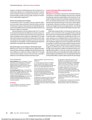
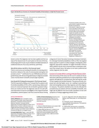
aseriesofbranchingsecondaryendpoints(Figure).
Steps in serial gatekeeping are as follows: (1) determine the or-
derfortestingmultipleendpoints,consideringtheirrelativeimpor-
tance and the likelihood that there is a difference in each; (2) test
the first end point against the desired global false-positive rate
(ie,.05)and,ifthefindingdoesnotreachstatisticalsignificance,then
stopallfurthertestinganddeclarethisandalldownstreamendpoints
nonsignificant. If testing the first end point is significant, then de-
clare this difference significant and proceed with the testing of the
nextendpoint;(3)testthenextendpointusingasignificancethresh-
old of .05; if not significant, stop all further testing and declare this
andalldownstreamendpointsnonsignificant.Ifsignificant,thende-
clare this difference significant and proceed with the testing of the
next end point; and (4) repeat the prior step until obtaining a first
nonsignificant result, or until all end points have been tested.
As shown in the Figure, this approach can be extended to test
2 or more end points at the same step by using a Bonferroni adjust-
ment to evenly split the false-positive error rate within the step. In
that case, testing is continued until either all branches have ob-
tainedafirstnonsignificantresultorallendpointshavebeentested.
Forexample,aneuroimagingendpointcouldbeusedasasingleend
pointforthefirstlevel,reflectingtheassumptionthatifanimprove-
ment in an imaging outcome is not achieved then an improvement
in a patient-centered functional outcome is highly unlikely, fol-
lowedbyasplittoallowthetestingofmotorfunctionsononebranch
and verbal functions on the other. This avoids the need to prioritize
eithermotororverbalfunctionovertheotherandmayincreasethe
ability to demonstrate an improvement in either domain.
Serialgatekeepingprovidesstrictcontrolofthefalse-positiveerror
ratebecauseitrestrictsmultiplecomparisonsbysequentiallytesting
hypothesesuntilthefirstnonsignificanttestisfound,and,nomatter
howsignificantlaterendpointsappeartobe,theyarenevertested.The
advantageisincreasedpowerfordetectingeffectsontheendpoints
thatappearearlyinthesequencebecausetheyaretestedagainst.05
rather than, eg, .05 divided by the total number of outcomes tested
usingatraditionalBonferroniadjustment.Byaccountingfortheimpor-
tanceofcertainhypothesesoverothersandbygroupinghypotheses
into primary and secondary groups, gatekeeping allocates the trial’s
power to be consistent with the investigators’ priorities.6
What Are the Limitations of Gatekeeping Strategies?
Gatekeeping strategies are a powerful way to incorporate trial-
specific clinical information to create prespecified ordering of hy-
potheses and mitigate the need to adjust for multiple comparisons
jama.com (Reprinted) JAMA October 10, 2017 Volume 318, Number 14 1385

ateachstageoftesting.Theprimarychallengeinusinggatekeeping
istheneedtoprespecifyandtrulycommittotheorderoftesting.The
resultinglimitationisthatif,inretrospect,theorderofoutcometest-
ing appears ill chosen (eg, if an early end point is negative and im-
portantendpointslaterinthesequenceappeartosuggestlargetreat-
ment effects), then there is no rigorous, post hoc method for
statistically evaluating the later end points. This highlights the im-
portance of having a clear data analysis strategy determined before
thetrialisstarted,andmaintainingtransparency(eg,publishingthe
study design and analysis plan on public websites or in journals).
How Was Gatekeeping Used in This Case?
TheCLEAN-TAVIinvestigatorsusedagatekeepingstrategytocom-
pare several magnetic resonance imaging end points along with
neurologicalandneurocognitiveperformance.1
Thefirstwasthepri-
marystudyendpoint,thenumberofbrainlesions2daysafterTAVI.
Secondaryendpointswereonlytestediftheprimaryonewasposi-
tive. Then, up to 16 secondary end points were tested in a defined
sequence. The study was markedly positive, with the primary and
manysecondaryendpointsdemonstratingbenefit.Thefirst8com-
parisonswerereportedindetailinthepublication—intheirprespeci-
fied order—retaining the structure of the gatekeeping strategy.1
The CLEAN-TAVI clinical trial demonstrated the efficacy of a cere-
bral protection strategy with respect to multiple imaging measures
ofischemicdamage.Theuseoftheprespecifiedgatekeepingstrat-
egyshouldprovideassurancethatthelargenumberofimagingend
points that were compared was unlikely to have led to false-
positive results.
ARTICLE INFORMATION
California (Yadav, Lewis); Los Angeles Biomedical
Research Institute, Torrance, California (Yadav);
Berry Consultants, LLC, Austin, Texas (Lewis).
Corresponding Author: Kabir Yadav, MDCM, MS,
MSHS, Department of Emergency Medicine,
1000 W Carson St, Box 21, Torrance, CA 90509
(kabir@emedharbor.edu).
none were reported.
REFERENCES
1. Haussig S, Mangner N, Dwyer MG, et al. Effect
of a cerebral protection device on brain lesions
following transcatheter aortic valve implantation in
patients with severe aortic stenosis. JAMA. 2016;
316(6):592-601.
2. Cao J, Zhang S. Multiple comparison procedures.
JAMA. 2014;312(5):543-544.
3. Bland JM, Altman DG. Multiple significance tests:
the Bonferroni method. BMJ. 1995;310(6973):170-
170.
4. Hommel G, Bretz F, Maurer W. Powerful
short-cuts for multiple testing procedures with
special reference to gatekeeping strategies. Stat Med.
2007;26(22):4063-4073.
5. Holm S. A simple sequentially rejective multiple
test procedure. Scand J Stat. 1979;6(2):65-70.
6. Dmitrienko A, Millen BA, Brechenmacher T,
Paux G. Development of gatekeeping strategies in
confirmatory clinical trials. Biom J. 2011;53(6):875-
893.
Figure. Criteria for Statistical Significance That Would Be Used in a Hypothetical Gatekeeping Strategy
Outcome 1 A vs B
A vs B
Outcome 2
A vs B
A vs B A vs B
Outcome 3
Outcome 4 Outcome 6
P<.05
P≥.05
P<.05
P<.025 P<.025
P<.05
Comparison not significant
Comparison significant
STOP
P≥.05
STOP
P≥.05
STOP
P≥.025
STOP
this
branch
A vs B A vs B
Outcome 5 Outcome 7
P<.025 P<.025
P≥.025
Comparison
not significant
P≥.025
STOP
this
branch
P≥.025
Comparison
not significant
This Figure shows the criteria for statistical significance that would be used in a
hypothetical gatekeeping strategy in which there are 3 levels each with a single
end point, followed by 2 levels with 2 end points each. The 3 end points are
each tested in order against a criterion of .05. All testing stops as soon as 1 result
is nonsignificant. If all are significant then a pair of fourth-level end points are
tested, and to preserve the required significance of .05 at that level across 2
end points, the criterion for statistical significance is adjusted with a Bonferroni
correction value of .025 for each. If 1 or both of these end points is significant at
.025, then the next end point in the branch is tested, against a criterion of .025.
If 1 or both are nonsignificant, no further testing occurs. If any outcome tested
along a given pathway is not statistically significant, no further outcomes along
that branch are tested because they are assumed to be nonsignificant.
1386 JAMA October 10, 2017 Volume 318, Number 14 (Reprinted) jama.com

Multiple Comparison Procedures
Jing Cao, PhD; Song Zhang, PhD
Problems can arise when researchers try to assess the statistical
significance of more than 1 test in a study. In a single test, statistical
significanceisoftendeterminedbasedonanobservedeffectorfind-
ing that is unlikely (<5%) to occur due to chance alone. When more
than 1 comparison is made, the chance of falsely detecting a non-
existent effect increases. This is known as the problem of multiple
comparisons(MCs),andadjustmentscanbemadeinstatisticaltest-
ing to account for this.1
In this issue of JAMA, Saitz et al2
report results of a randomized
trialevaluatingtheefficacyof2briefcounselinginterventions(ie,a
brief negotiated interview and an adaptation of a motivational in-
terview, referred to as MOTIV) in reducing drug use in primary care
patients when compared with
not having an intervention. Be-
cause MCs were made, the au-
thors adjusted how they determined statistical significance. In this
article,weexplainwhyadjustmentforMCsisappropriateinthisstudy
and point out the limitations, interpretations, and cautions when
using these adjustments.
Use of Method
Why Are Multiple Comparison Procedures Used?
Whenasinglestatisticaltestisperformedatthe5%significancelevel,
thereisa5%chanceoffalselyconcludingthatasupposedeffectex-
ists when in fact there is none. This is known as making a false dis-
coveryorhavingafalse-positiveinference.Thesignificancelevelrep-
resents the risk of making a false discovery in an individual test,
denoted as the individual error rate (IER). If 20 such tests are con-
ducted,thereisa5%chanceofmakingafalse-positiveinferencewith
each test so that, on average, there will be 1 false discovery in the
20 tests.
Anotherwaytoviewthisisintermsofprobabilities.Iftheprob-
ability of making a false conclusion (ie, false discovery) is 5% for a
single test in which the effect does not exist, then 95% of the time,
the test will arrive at the correct conclusion (ie, insignificant effect).
With2suchtests,theprobabilityoffindinganinsignificanteffectwith
the first test is 95%, as it is for the second. However, the probability
of finding insignificant effects in the first and the second test is
0.95 × 0.95, or 90%. With 20 such tests, the probability that all of
the20testscorrectlyshowinsignificanceis(0.95)20
or36%.Sothere
is a 100% − 36%, or 64%, chance of at least 1 false-positive test oc-
curring among the 20 tests. Because this probability quantifies the
risk of making any false-positive inference by a group, or family, of
tests, it is referred to as the family-wise error rate (FWER). The
FWER generally increases as the number of tests performed in-
creases.Forexample,assumingIER = 5%anddenotingthenumber
of multiple tests performed as K, then for K = 2 independent tests,
FWER = 1 − (0.95)2
= 10%;forK = 3,FWER = 1 − (0.95)3
= 14%;and
for K = 20, FWER = 1 − (0.95)20
= 64%. This shows that the risk of
making at least 1 false discovery in MCs can be greatly inflated even
if the error rate is well controlled in each individual test.
When MCs are made, to control FWER at a certain level, the
threshold for determining statistical significance in individual tests
must be adjusted.1
The simplest approach is known as the Bonfer-
ronicorrection.Itadjuststhestatisticalsignificancethresholdbythe
number of tests. For example, for a FWER fixed at 5%, the IER in a
group of 20 tests is set at 0.05/20 = 0.0025; ie, an individual test
would have to have a P value less than .0025 to be considered sta-
tistically significant. The Bonferroni correction is easy to imple-
ment, but it sets the significance threshold too rigidly, reducing the
statistical procedure’s power to detect true effects.
The Hochberg sequential procedure, which was used in the
studybySaitzetal,2
takesadifferentapproach.3
Allofthetests(the
multiplecomparisons)areperformedandtheresultantPvaluesare
ordered from largest to smallest on a list. If the FWER is fixed at 5%
and the largest observed P value is less than .05, then all the tests
are considered significant. Otherwise, if the next largest P value is
less than 0.05/2 (.025), then all the tests except the one with the
largestPvalueareconsideredsignificant.Ifnot,andthethirdPvalue
in the list is less than 0.05/3 (.017), then all the tests except those
withthelargest2Pvaluesareconsideredsignificant.Thisiscontin-
ueduntilallthecomparisonsaremade.Thisapproachusesprogres-
sively more stringent statistical thresholds with the most stringent
one being the Bonferroni threshold, and thus the approach can
achieve a greater power to detect true effect than the Bonferroni
procedure under appropriate conditions. An example in the Table
consists of 6 tests in MCs; given a FWER of 5%, none of the tests
Table. An Example to Compare the Bonferroni Procedure and the Hochberg Sequential Procedure
Test P Value
Bonferroni Hochberg
Threshold Result Threshold Result
1 .40 0.05/6 = 0.008 Not significant 0.05 Not significant
2 .027 0.05/6 = 0.008 Not significant 0.05/2 = 0.025 Not significant
3 .020 0.05/6 = 0.008 Not significant 0.05/3 = 0.017 Not significant
4 .012 0.05/6 = 0.008 Not significant 0.05/4 = 0.0125 Significant
5 .011 0.05/6 = 0.008 Not significant NA Significant
6 .010 0.05/6 = 0.008 Not significant NA Significant
Abbreviation: NA, not applicable.
jama.com JAMA August 6, 2014 Volume 312, Number 5 543

aresignificantwiththeBonferroniprocedure.Bycomparison,3tests
are significant with the Hochberg sequential procedure.
What Are the Limitations of Multiple Comparison Procedures?
Statistical procedures to control FWER in MCs were developed to
reduce the risk of making any false-positive discovery. This is offset
by having a lower test power to detect true effects. For example,
when K = 10, the Bonferroni-corrected IER is 0.05/10 = 0.005 to
control FWER at 0.05. Under the conventional 2-sided t test, for a
single test in the group to be considered significant, the observed
effect needs to be 43% larger than that with an IER = 0.05. When
K = 20,theBonferroni-correctedIERis0.05/20 = 0.0025,andthe
observedeffectneedstobe54%largerthanthatwithanIER = 0.05.
This limitation of reduced test power by controlling FWER be-
comes more apparent as the number of tests in MCs increases.
Why Did the Authors Use Multiple Comparison Procedures
In the study by Saitz et al, 2 tests were performed (brief negotiated
interview vs no brief interview and MOTIV vs no brief interview) to
determineifinterventionswithbriefcounselingweremoreeffective
in reducing drug use than interventions without counseling. With 2
testsandtheIERsetat5%,theriskoffalselyconcludingatleast1treat-
ment is effective because of chance alone is 10%. To avoid the in-
flatedFWER,theauthorsusedtheHochbergsequentialprocedure.3
How Should This Method’s Findings Be Interpreted
Saitz et al found that the adjusted P value4
based on the Hoch-
berg procedure was .81 for both the brief negotiated interview
and MOTIV vs no brief interview. The study did not provide suffi-
cient evidence to claim that interventions with brief counseling
were more effective than the one without brief counseling in
reducing drug use among primary care patients. However, the
absence of evidence does not mean there is an absence of an
effect. The interventions may be effective, but this study did not
have the statistical power to detect the effect.
Caveats to Consider When Looking at Multiple Comparison
Procedures
To Adjust or Not
If researchers conduct multiple tests, each addressing an unre-
lated research question, then adjusting for MCs is unnecessary.
Suppose in a different study, brief negotiated interview was
intended to treat alcohol use and MOTIV was intended to treat
drug use. Then there is no need to adjust for MCs. This is in con-
trast to performing a family of tests from which the results as a
whole address a single research question; then adjusting for MCs
is necessary. As in the report by Saitz et al,2
both the brief negoti-
ated interview and MOTIV were compared with the control to
draw a single conclusion about the efficacy of brief counseling
interventions for drug use.
Confirmatory vs Exploratory
Bender and Lange5
suggested that MC procedures are only
required for confirmatory studies for which the goal is the defini-
tive proof of a predefined hypothesis to support final decision
making. For exploratory studies seeking to generate hypotheses
that will be tested in future confirmatory studies, the number of
tests is usually large and the choice of hypotheses is likely data
dependent (ie, selecting hypotheses after reviewing data), mak-
ing MC adjustments unnecessary or even impossible at this stage
of research. “Significant” results based on exploratory studies,
however, should be clearly labeled so readers can correctly assess
their scientific strength.
FWER vs FDR
The main approaches to MC adjustment include controlling
FWER, which is the probability of making at least 1 false discovery
in MCs, or controlling the false discovery rate (FDR), which is the
expected proportion of false positives among all discoveries.
When using the FDR approaches, a small proportion of false posi-
tives are tolerated to improve the chance of detecting true
effects.6
In contrast, the FWER approaches avoid any false posi-
tives even at the cost of increased false negatives. The FDR and
FWER represent 2 extremes of the relative importance of control-
ling for false positive or false negatives. The decision whether to
control FWER or FDR should be made by carefully weighing the
relative benefits between false-positive and false-negative dis-
coveries in a specific study.
Definition of Family
BothFWERandFDRaredefinedforaparticularfamilyoftests.This
“family” should be prespecified at the design stage of a study. Test
bias can occur in MCs when selecting hypothesis to be tested after
reviewing the data.
ARTICLE INFORMATION
Author Affiliations: Department of Statistical
Science, Southern Methodist University, Dallas,
Texas (Cao); Department of Clinical Sciences,
UT Southwestern Medical Center, Dallas, Texas
(Zhang).
Corresponding Author: Jing Cao, PhD, Southern
Methodist University, Statistical Science, Dallas, TX
75205 (jcao@smu.edu).
none were reported.
REFERENCES
1. Hsu JC. Multiple Comparisons: Theory and
Methods. London, UK: Chapman & Hall; 1996.
2. Saitz R, Palfai TPA, Cheng DM, et al. Screening
and brief intervention for drug use in primary care:
the ASPIRE randomized clinical trial. JAMA. doi:10
.1001/jama.2014.7862.
3. Hochberg Y. A sharper Bonferroni procedure for
multiple tests of significance. Biometrika. 1988;75
(4):800-802.
4. Wright SP. Adjusted P value for simultaneous
inference. Biometrics. 1992;48(4):1005-1013.
5. Bender R, Lange S. Adjusting for multiple
testing: when and how? J Clin Epidemiol. 2001;54
(4):343-349.
6. Benjamini Y, Hochberg Y. Controlling the false
discovery rate: a practical and powerful approach to
multiple testing. J R Stat Soc B. 1995;57(1):289-300.
544 JAMA August 6, 2014 Volume 312, Number 5 jama.com

Pragmatic Trials
Practical Answers to “Real World” Questions
Harold C. Sox, MD; Roger J. Lewis, MD, PhD
Theconceptofa“pragmatic”clinicaltrialwasfirstproposednearly
50yearsagoasastudydesignphilosophythatemphasizesanswer-
ing questions of most interest to decision makers.1
Decision mak-
ers, whether patients, physi-
cians, or policy makers, need to
knowwhattheycanexpectfrom
theavailablediagnosticorthera-
peutic options when applied in day-to-day clinical practice. This fo-
cus on addressing real-world effectiveness questions influences
choices about trial design, patient population, interventions, out-
comes, and analysis. In this issue of JAMA, Gottenberg et al2
report
the results of a trial designed to answer the question “If a biologic
agent for rheumatoid arthritis is no longer effective for an indi-
vidual patient, should the clinician recommend another drug with
the same mechanism of action or switch to a biologic with a differ-
entmechanismofaction?”Becausetheauthorsincludedsomeprag-
maticelementsinthetrialdesign,thisstudyillustratestheissuesthat
clinicians should consider in deciding whether a trial result is likely
to apply to their patients.
Use of the Method
Why Are Pragmatic Trials Conducted?
Pragmatic trials are intended to help typical clinicians and typical
patients make difficult decisions in typical clinical care settings by
maximizing the chance that the trial results will apply to patients
that are usually seen in practice (external validity). The most impor-
tant feature of a pragmatic trial is that patients, clinicians, clinical
practices, and clinical settings are selected to maximize the applica-
bility of the results to usual practice. Trial procedures and require-
ments must not inconvenience patients with substantial data col-
lection and should impose a minimum of constraints on usual
practice by allowing a choice of medication (within the constraints
imposed by the purpose of the study) and dosage, providing the
freedom to add cointerventions, and doing nothing to maximize
adherence to the study protocol.
The pragmatic trial strategy contrasts with that used for an
explanatory trial, the goal of which is to test a hypothesis that the
intervention causes a clinical outcome. Explanatory trials seek to
maximize the probability that the intervention—and not some
other factor—causes the study outcome (internal validity). Explana-
tory trials seek to give the intervention the best possible chance to
succeed by using experts to deliver it, delivering the intervention to
patients who are most likely to respond, and administering the
intervention in settings that provide expert after-care. Explanatory
trials try to prevent any extraneous factors from influencing clinical
outcomes, so they exclude patients who might have poor adher-
ence and may intervene to maximize patient and clinician adher-
ence to the study protocol. Explanatory trials are structured to
avoid downstream events that could affect study outcomes. If
these events occur at different rates in the different study groups,
the effect attributed to the intervention may be larger or smaller
than its true effect. To avoid this problem, explanatory trials may
choose a relatively short follow-up period. Explanatory trials pur-
sue internal validity at the cost of external validity, whereas prag-
matic trials place a premium on external validity while maintaining
as much internal validity as possible.
Description of the Method
According to Tunis et al,3
“the characteristic features of [prag-
matic clinical trials] are that they (1) select clinically relevant alter-
native interventions to compare, (2) include a diverse population
of study participants, (3) recruit participants from heterogeneous
practice settings, and (4) collect data on a broad range of health
outcomes.” Eligible patients may be defined by presumptive diag-
noses, rather than confirmed ones, because treatments are often
initiated when the diagnosis is uncertain.3
Pragmatic trials may
compare classes of drugs and allow the physician to choose which
drug in the class to use, the dose, and any cointerventions, a free-
dom that mimics usual practice. Furthermore, the outcome mea-
sures are more likely to be patient-reported, global, subjective,
and patient-centered (eg, self-reported quality-of-life measures),
rather than the more disease-centered end points commonly
used in explanatory trials (eg, the results of laboratory tests or
imaging procedures).
Bothapproachestostudydesignmustdealwiththecostofclini-
cal trials. Explanatory trials control costs by keeping the trial period
as short as possible, consistent with the investigators’ ability to en-
rollenoughpatientstoanswerthestudyquestion.Thesetrialspref-
erentially recruit patients who will experience the study end point
and not leave the study early because of disinterest or death from
causes other than the target condition. Investigators in explana-
tory trials prefer to enroll participants with a high probability of ex-
periencinganoutcomeinthenearterm.Incontrast,pragmatictrials
maycontrolcostsbyleveragingexistingdatasources,eg,usingdis-
easeregistriestoidentifypotentialparticipantsandusingdatainelec-
tronic health records to identify study outcomes.
Althoughtheseconceptssharpenthecontrastsbetweenprag-
maticandexplanatorytrialsforpedagogicalreasons,inreality,many
trials have features of both designs, in part to find a reasonable bal-
ance between internal validity and external validity.4,5
What Are the Limitations of Pragmatic Trials?
The main limitation of a pragmatic trial is a direct consequence of
choosing to conduct a lean study that puts few demands on
patients and clinicians. Data collection may be sparse, and there are
few clinical variables with which to identify subgroups of patients

who respond particularly well to one of the interventions. The use
of the electronic health record as a source of data may save money,
but it typically means inconsistent data collection and missing data.
Relying on typical clinicians rather than experts in caring for
patients with the target condition may lead to increased variability
in practice and associated documentation of clinical findings. The
variation caused by these shortcomings may reduce statistical pre-
cision and the capability of answering the research question
unequivocally.
Why Was a Pragmatic Trial Conducted in This Case?
WhileGottenberetal2
citethepragmatismoftheirstudyasitsmain
strength, the authors do not explain their study design decisions.
However, they imply a pragmatic motivation when they state that
thestudyconfirmsthesuperiorityofadrugfromadifferentclassin
asettingthat“correspondstothetherapeuticquestioncliniciansface
in daily practice.” The investigators note that their main limitation
of the study was the inability to blind the participants to the iden-
tityofthedrugtheyreceived.Blindingisespeciallyimportantwhen
theprincipalstudyoutcomesarethosereportedbythepatient,who
may be influenced by knowing the intervention that they received.
The study by Gottenberg et al2
shows that, from the perspective of
a population of patients, changing from one class of drugs to an-
other improves the outcomes of care by rheumatologists in a rheu-
matology subspecialty clinic. This result has limited external valid-
ity. It probably applies to other rheumatology clinics, but its
application to other settings is unknown. The main pragmatic fea-
ture of the study—allowing the rheumatologist to choose from sev-
eraldrugswithinaclass—impliesthatthemainresultappliesstrictly
totheclassofdrugsratherthantoanyindividualagent.Itdoesnot,
for example, show that the improvement is the same regardless of
which within-class drug the clinician determines. The trial was also
pragmaticinthatclinicianswereawareoftheprimarytreatmentand
were free to choose cointerventions that would complement it, as
would occur in clinical practice.
Several features of this study were not pragmatic, and others
raise internal validity concerns. The researchers recruited partici-
pants from rheumatology specialty clinics. Although the article
does not specify the clinicians who managed the patient’s rheu-
matoid arthritis during the study, the clinicians were presumably
rheumatologists in the participating practices. Even though the
results apply to patients in a specialty clinic, whether they apply
to patients managed by primary care physicians, with or without
expert consultation, is unknown. The authors also did not specify
the intensity of follow-up; was it typical of rheumatoid arthritis
patients receiving biologic agents or did the study protocol
specify more intensive follow up? The primary outcome measure
was a score based on the erythrocyte sedimentation rate and a
count of involved joints. The article does not identify the person
who assessed the primary outcome. Assigning this task to the
managing physician would be consistent with a pragmatic design,
but it would also raise concerns about biased outcome assess-
ment because the person measuring the outcome would know
the treatment assignment.
The terms “explanatory” and “pragmatic” mark the ends of
a spectrum of study designs. Typically, as noted by Thorpe and
co-authors of the PRECIS (Pragmatic-Explanatory Continuum Indi-
catorSummary)article,5
somefeaturesofastudyarepragmaticand
others are explanatory, as the study by Gottenberg et al illustrates
andaswouldbeexpectedbecauseinternalvalidityandexternalva-
lidity are typically achieved at the cost of one another. Whether the
authorslabeltheirstudyaspragmaticorexplanatory,readersshould
paycloseattentiontothestudycharacteristicsthatmaximizeitsap-
plicability to their patients and their practice style.
ARTICLE INFORMATION
Author Affiliations: Patient Centered Outcomes
Research Institute (PCORI), Washington, DC (Sox);
Geisel School of Medicine at Dartmouth, Hanover,
New Hampshire (Sox); Department of Emergency
California (Lewis); Department of Emergency
Medicine, David Geffen School of Medicine at the
University of California-Los Angeles (Lewis); Berry
Consultants, LLC, Austin, Texas (Lewis).
Medical Center, 1000 W Carson St, PO Box 21,
none were reported.
Disclaimer: Dr Sox is an employee of the
Patient-Centered Outcomes Research Institute
(PCORI). This article does not represent the
policies of PCORI.
REFERENCES
1. Schwartz D, Lellouch J. Explanatory and
pragmatic attitudes in therapeutical trials. J Chronic
Dis. 1967;20(8):637-648.
2. Gottenberg J-E, Brocq O, Perdriger A, et al.
Non–TNF-targeted biologic vs a second anti-TNF
drug to treat rheumatoid arthritis in patients with
insufficient response to a first anti-TNF drug. JAMA.
doi:10.1001/jama.2016.13512
3. Tunis SR, Stryer DB, Clancy CM. Practical clinical
trials: increasing the value of clinical research for
decision making in clinical and health policy. JAMA.
2003;290(12):1624-1632.
4. Zwarenstein M, Treweek S, Gagnier JJ, et al;
CONSORT group; Pragmatic Trials in Healthcare
(Practihc) group. Improving the reporting of
pragmatic trials: an extension of the CONSORT
statement. BMJ. 2008;337:a2390. doi:10.1136/bmj
.a2390
5. Thorpe KE, Zwarenstein M, Oxman AD, et al.
A Pragmatic-Explanatory Continuum Indicator
Summary (PRECIS): a tool to help trial designers.
J Clin Epidemiol. 2009;62(5):464-475.

Equipoise in Research
Integrating Ethics and Science in Human Research
Alex John London, PhD
Theprincipleofequipoisestatesthat,whenthereisuncertaintyor
conflictingexpertopinionabouttherelativemeritsofdiagnostic,pre-
vention, or treatment options, allocating interventions to individu-
als in a manner that allows the
generation of new knowledge
(eg, randomization) is ethically
permissible.1,2
The principle of
equipoisereconciles2potentiallyconflictingethicalimperatives:to
ensurethatresearchinvolvinghumanparticipantsgeneratesscien-
tificallysoundandclinicallyrelevantinformationwhiledemonstrat-
ing proper respect and concern for the rights and interests of
study participants.1
In this issue of JAMA, Lascarrou et al3
report the results of a
randomized trial designed to investigate whether the “routine use
of the video laryngoscope for orotracheal intubation of patients in
the ICU increased the frequency of successful first-pass intubation
compared with use of the Macintosh direct laryngoscope.” Intuba-
tion in the intensive care unit (ICU) is associated with the potential
for serious adverse events, and video laryngoscopy in the ICU has
gained support from some clinicians who believe it to be superior
to direct laryngoscopy. Such practitioners may therefore regard it
as unethical to randomize study participants to direct laryngoscopy
because they consider it to be an inferior intervention. But requir-
ing uncertainty of individual clinicians to conduct a clinical trial
gives too much ethical weight to personal judgment, hindering
valuable research without providing benefit to patients. Therefore,
it is important to understand the role of conflicting expert medical
judgment in establishing equipoise and how this principle applies
to the trial conducted by Lascarrou et al.
What Is Equipoise?
Two features of medical research pose special challenges for the
goal of ensuring respect and concern for the rights and interests
of participants. First, to generate reliable information, research
often involves design features that alter the way participants are
treated. For example, randomization and blinding are commonly
used to reduce selection bias and treatment bias.4
Controlling
how interventions are allocated and what researchers and partici-
pants know about who is receiving which interventions helps to
more clearly distinguish the effects of the intervention from con-
founding effects. But randomization severs the link between
what a participant receives and the recommendation of a treating
clinician with an ethical duty to provide the best possible care for
the individual person. In the study by Lascarrou et al,3
patients
were randomized to undergo intubation with the video laryngo-
scope or the direct laryngoscope, independent of the preference
of the treating physician.
Second, medical research involves exposing people to inter-
ventionswhoserisksandpotentialtherapeutic,prophylactic,ordi-
agnosticmeritsmaybeunknown,unclear,orthesubjectofdisagree-
ment within the medical community. In the present case, some
cliniciansmaymaintainthatvideolaryngoscopyisthesuperiorstrat-
egyfororotrachealintubationintheICU,othersmaydisagree,while
othersjudgethatthereisnotsufficientevidencetowarrantastrong
commitment for or against this approach.
The principle of equipoise states that if there is uncertainty or
conflicting expert opinion about the relative therapeutic, prophy-
lactic, or diagnostic merits of a set of interventions, then it is per-
missibletoallocateaparticipanttoreceiveaninterventionfromthis
set, so long as there is not consensus that an alternative interven-
tion would better advance that participant’s interests.1,2,5-7
In the present case, there is equipoise between video vs di-
rect laryngoscopy because experts disagree about their relative
clinical merits. These disagreements are reflected in variations
in clinical practices. If it is ethically permissible for patients to
receive care from expert clinicians in good professional standing
with differing medical opinions about what constitutes optimal
treatment, then it ordinarily cannot be wrong to permit partici-
pants to be randomized to those same treatment alternatives.5
Although randomization removes the link between what a partici-
pant receives and the recommendation of a particular clinician, the
presence of equipoise ensures that each participant receives an
intervention that would be recommended or utilized by at least a
reasonable minority of informed expert clinicians.1,5,6
Equipoise
thus ensures that randomization is consistent with respect for par-
ticipant interests because it guarantees that no participant receives
care known to be inferior to any available alternative.
Why Is Equipoise Important?
Ensuring equipoise helps researchers and institutional review
boards (IRBs) fulfill 3 ethical obligations. First, to “disturb” equi-
poise studies must be designed to generate information that
resolves uncertainty or reduces divergence in opinion among quali-
fied medical experts. Such studies are likely to have both social and
scientific value. Second, any risks to which participants are exposed
must be reasonable in light of the value of the information a study
is likely to produce.5,6
IRBs must make this determination before
participants are enrolled.
Third is the obligation to show respect for potential partici-
pants as autonomous decision makers. Explaining during the
informed consent process the nature of the uncertainty or con-
flict in medical judgment that a study is designed to resolve
allows each individual to decide whether to participate by under-
standing the relevant uncertainties, their effects on that person’s
own interests, and how their resolution will contribute to improv-
ing the state of medical care.
What Are the Limitations of Equipoise?
Since its introduction, the concept of equipoise has received nu-
merous formulations, creating the potential for confusion and
jama.com (Reprinted) JAMA February 7, 2017 Volume 317, Number 5 525

misunderstanding2,7
and spurring criticism and debate. One criti-
cism holds that the version of equipoise described here is too per-
missive because it allows randomization even when individual cli-
niciansarenotuncertainabouthowbesttotreatapatient.8
Thetrial
conducted by Lascarrou et al3
represents a case in which some cli-
nicianshavestrongpreferencesforonemodalityoftreatmentover
others.Requiringindividualclinicianuncertaintyentrenchesunwar-
rantedvariationinpatientcarebypreventingparticipantsfrombeing
offeredthechoiceofparticipatinginastudyinwhichtheymightbe
allocated to interventions that would be recommended or utilized
by other medical experts. If it is ethically acceptable for patients to
receivecarefrominformed,expertclinicianswhofavordifferentin-
terventions, then it ordinarily cannot be unethical to allow patients
to be randomized to the alternatives that such clinicians recom-
mend. Legitimate disagreement among informed experts signifies
thattheclinicalcommunitylacksabasisforjudgingthatpatientsare
better off with one modality over the other.
Aninterpretationofequipoisethatrequiresuncertaintyonthe
partoftheindividualclinicianisnotethicallyjustifiedbecauseitpre-
vents studies that are likely to improve the quality of patient care
without the credible expectation that this restriction will improve
patient outcomes.
Anothercriticismisthatequipoiseisunlikelyevertoexist,orto
persistforlong.9
Thisobjectionappliesmostdirectlytotheviewthat
equipoise only exists if the individual clinician believes that the in-
terventions offered in a trial are of exactly equal expected value.10
On this view, equipoise would often disappear even though differ-
ent experts retain conflicting medical recommendations.
Itthereforeappearspoorlysuitedtothegoalsofpromotingthepro-
duction of valuable information and protecting the interests of
study participants.
How Is Equipoise Applied in This Case?
Lascarrouetaldidnotexplicitlydiscussequipoiseintheirstudy.How-
ever, the consent process approved by the ethics committee re-
flects the judgment that the interventions in the trial “were consid-
ered components of standard care” and patients who lacked
decisional capacity could be enrolled even if no surrogate decision
maker was present.
Ensuringthatastudybeginsinandisdesignedtodisturbastate
of equipoise provides credible assurance to participants and other
stakeholders that patients in medical distress can be enrolled in a
studythatwillhelpimprovepatientcareinemergencysettingswith-
out concern that their health interests will be knowingly compro-
mised in the process.
How Does Equipoise Influence the Interpretation
of the Study?
In the past, strongly held beliefs about the effectiveness of treat-
ments ranging from bloodletting to menopausal hormone therapy
have proven to be false. Intubation in the ICU is associated with
the potential for serious adverse events. Because video laryngos-
copy is increasingly championed as the superior method for orotra-
cheal intubation in the ICU, careful study of its relative merits and
risks in comparison to conventional direct laryngoscopy addresses
a question of clinical importance. The findings of Lascarrou et al3
suggest that perceived merits of video laryngoscopy do not trans-
late into superior clinical outcomes and may be associated with
higher rates of life-threatening complications. This result under-
scores the importance of conducting clinical research before novel
interventions become widely incorporated into clinical practice,
even if those interventions appear to offer clear advantages over
existing alternatives.
ARTICLE INFORMATION
Author Affiliation: Department of Philosophy,
Carnegie Mellon University, Pittsburgh,
Pennsylvania.
Corresponding Author: Alex John London, PhD,
Department of Philosophy, Center for Ethics
and Policy, Carnegie Mellon University,
135 Baker Hall, Pittsburgh, PA 15213-3890
(ajlondon@andrew.cmu.edu).
none were reported.
REFERENCES
1. Freedman B. Equipoise and the ethics of clinical
research. N Engl J Med. 1987;317(3):141-145.
2. London AJ. Clinical equipoise: foundational
requirement or fundamental error? In: Steinbock B,
ed. The Oxford Handbook of Bioethics. Oxford, UK:
Oxford University Press; 2007:571-595.
3. Lascarrou JB, Boisrame-Helms J, Bailly A, et al;
Clinical Research in Intensive Care and Sepsis
(CRICS) Group. Video laryngoscopy vs direct
laryngoscopy on successful first-pass orotracheal
intubation among ICU patients: a randomized
clinical trial. JAMA. doi:10.1001/jama.2016.20603
4. Guyatt G, Rennie D, Meade MO, Cook DJ. Users’
Guides to the Medical Literature: A Manual for
Evidence-Based Clinical Practice. 3rd ed. New York,
NY: McGraw-Hill; 2015.
5. London AJ. Reasonable risks in clinical research:
a critique and a proposal for the Integrative
Approach. Stat Med. 2006;25(17):2869-2885.
6. Miller PB, Weijer C. Rehabilitating equipoise.
Kennedy Inst Ethics J. 2003;13(2):93-118.
7. van der Graaf R, van Delden JJ. Equipoise should
be amended, not abandoned. Clin Trials. 2011;8(4):
408-416.
8. Hellman D. Evidence, belief, and action: the
failure of equipoise to resolve the ethical tension in
the randomized clinical trial. J Law Med Ethics.
2002;30(3):375-380.
9. Sackett DL. Equipoise, a term whose time
(if it ever came) has surely gone. CMAJ. 2000;163
(7):835-836.
10. Lilford RJ, Jackson J. Equipoise and the ethics
of randomization. J R Soc Med. 1995;88(10):552-559.
526 JAMA February 7, 2017 Volume 317, Number 5 (Reprinted) jama.com

The Propensity Score
Jason S. Haukoos, MD, MSc; Roger J. Lewis, MD, PhD
Two recent studies published in JAMA involved the analysis of ob-
servationaldatatoestimatetheeffectofatreatmentonpatientout-
comes. In the study by Rozé et al,1
a large observational data set was
analyzed to estimate the relationship between early echocardio-
graphic screening for patent ductus arteriosus and mortality among
preterm infants. The authors compared mortality rates of 847 in-
fants who were screened for patent ductus arteriosus and 666 who
were not. The 2 infant groups were dissimilar; infants who were
screenedwereyounger,morelikelyfemale,andlesslikelytohavere-
ceived corticosteroids. The authors used propensity score matching
tocreate605matchedinfantpairsfromtheoriginalcohorttoadjust
forthesedifferences.InthestudybyHuybrechtsetal,2
theMedicaid
AnalyticeXtractdatasetwasanalyzedtoestimatetheassociationbe-
tween antidepressant use during pregnancy and persistent pulmo-
nary hypertension of the newborn. The authors included 3 789 330
women, of which 128 950 had used antidepressants. Women who
used antidepressants were different from those who had not, with
differences in age, race/ethnicity, chronic illnesses, obesity, tobacco
use, and health care use. The authors adjusted for these differences
using, in part, the technique of propensity score stratification.
Use of the Method
Why Were Propensity Methods Used?
Many considerations influence the selection of one therapy over an-
other.Inmanysettings,morethanonetherapeuticapproachiscom-
monly used. In routine clinical practice, patients receiving one treat-
ment will tend to be different from those receiving another, eg, if
onetreatmentisthoughttobebettertoleratedbyelderlypatientsor
moreeffectiveforpatientswhoaremoreseriouslyill.Thisresultsina
correlation—or confounding—between patient characteristics that
affectoutcomesandthechoiceoftherapy(oftencalled“confounding
byindication”).Ifobservationaldataobtainedfromroutineclinicalprac-
ticeareexaminedtocomparetheoutcomesofpatientstreatedwith
differenttherapies,theobserveddifferencewillbetheresultofboth
differingpatientcharacteristicsandtreatmentchoice,makingitdiffi-
cult to delineate the true effect of one treatment vs another.
The effect of an intervention is best assessed by randomizing
treatment assignments so that, on average, the patients are similar
inthe2treatmentgroups.Thisallowsadirectassessmentoftheef-
fect of the intervention on outcome. In observational studies, ran-
domization is not possible, so investigators must adjust for differ-
encesbetweengroupstoobtainvalidestimatesoftheassociations
between the treatments being compared and the outcomes of
interest.3
Multivariable statistical methods are often used to esti-
mate this association while adjusting for confounding.
Propensityscoremethodsareusedtoreducethebiasinestimat-
ingtreatmenteffectsandallowinvestigatorstoreducethelikelihood
ofconfoundingwhenanalyzingnonrandomized,observationaldata.
Thepropensityscoreistheprobabilitythatapatientwouldreceivethe
treatmentofinterest,basedoncharacteristicsofthepatient,treating
clinician,andclinicalenvironment.4
Suchprobabilitiescanbeestimated
using multivariable statistical methods (eg, logicistic regression), in
which case the treatment of interest is the dependent variable and
thecharacteristicsofthepatient,prescribingclinician,andclinicalset-
tingarethepredictors.Investigatorsestimatetheseprobabilities,rang-
ing from 0 to 1, for each patient in the study population. These
probabilities—the propensity scores—are then used to adjust for dif-
ferencesbetweengroups.Inbiomedicalstudies,propensityscoresare
oftenusedtocomparetreatments,buttheycanalsobeusedtoesti-
matetherelationshipbetweenanynonrandomizedfactor,suchasthe
exposure to a toxin or infectious agent and the outcome of interest.
Thereare4generalwayspropensityscoresareused.Themost
common is propensity score matching, which involves assembling
2 groups of study participants, one group that received the treat-
ment of interest and the other that did not, while matching indi-
viduals with similar or identical propensity scores.1
The analysis of
a propensity score–matched sample can then approximate that of
a randomized trial by directly comparing outcomes between indi-
viduals who received the treatment of interest and those who did
not, using methods that account for the paired nature of the data.5
Thesecondapproachisstratificationonthepropensityscore.4
This
technique involves separating study participants into distinct groups
or strata based on their propensity scores. Five strata are commonly
used, although increasing the number can reduce the likelihood of
bias. The association between the treatment of interest and the
outcome of interest is estimated within each stratum or pooled
across strata to provide an overall estimate of the relationship be-
tweentreatmentandoutcome.Thistechniquereliesonthenotionthat
individualswithineachstratumaremoresimilartoeachotherthanin-
dividuals in general; thus, their outcomes can be directly compared.
The third approach is covariate adjustment using the propen-
sity score. For this approach, a separate multivariable model is de-
veloped, after the propensity score model, in which the study out-
comeservesasthedependentvariableandthetreatmentgroupand
propensityscoreserveaspredictorvariables.Thisallowstheinves-
tigator to estimate the outcome associated with the treatment of
interest while adjusting for the probability of receiving that treat-
ment, thus reducing confounding.
Thefourthapproachisinverseprobabilityoftreatmentweight-
ing using the propensity score.6
In this instance, propensity scores
are used to calculate statistical weights for each individual to cre-
ateasampleinwhichthedistributionofpotentialconfoundingfac-
tors is independent of exposure, allowing an unbiased estimate of
the relationship between treatment and outcome.7
Alternative strategies—other than use of propensity scores—
for adjusting for baseline differences between groups in observa-
tionalstudiesincludematchingonbaselinecharacteristics,perform-
ing stratified analyses, or using multivariable statistical methods to
adjust for confounders. Propensity score methods are often more
practical or statistically more efficient than these methods, in part
jama.com (Reprinted) JAMA October 20, 2015 Volume 314, Number 15 1637

becausepropensityscoremethodscansubstantiallylimitthenum-
berofpredictorvariablesusedinthefinalanalysis.Propensityscore
methods generally allow many more variables to be included in the
propensity score model, which increases the ability of these ap-
proachestoeffectivelyadjustforconfounding,thancouldbeincor-
porated directly into a multivariable analysis of the study outcome.
What Are the Limitations of Propensity Score Methods?
Thepropensityscoreforeachstudyparticipantisbasedontheavail-
able measured patient characteristics, and unadjusted confounding
may still exist if unmeasured factors influenced treatment selection.
Therefore,usingfewervariablesinthepropensityscoremodelreduces
the likelihood of effectively adjusting for confounding.
Although propensity score matching may be used to assemble
comparable study groups, the quality of matching depends on the
quality of the propensity score model, which in turn depends on
thequalityandsizeoftheavailabledataandhowthemodelwasbuilt.
Conventional modeling methods (eg, variable selection, use of in-
teractions, regression diagnostics, etc) are not typically recom-
mended for the development of propensity score models. For ex-
ample, propensity score models may optimally include a larger
number of predictor variables.
Why Did the Authors Use Propensity Methods?
InthereportsbyRozéetal1
andHuybrechtsetal,2
bothofwhomused
propensityscoremethodsbecausetheirdatawereobservational,the
treatmentsofinterest(ie,screeningbyechocardiographyanduseof
antidepressantsinpregnancy)werenotrandomlyallocated,andim-
portantcharacteristicsdifferedbetweengroups.Directcomparisons
oftheoutcomesbetweentreatedanduntreatedgroupswouldhave
likelyresultedinsignificantlybiasedestimates.Instead,useofpropen-
sityscorematchingandstratificationenabledtheinvestigatorstocre-
atestudygroupsthatweresimilartooneanotherandmoreaccurately
measure the relationship between treatment and outcome.
How Should the Findings Be Interpreted?
Given the observational nature of these studies, the fact that indi-
vidualsinthetreatedanduntreatedgroupsweredissimilar,andthe
goalofaccuratelyestimatingtheassociationbetweentreatmentand
outcome,theinvestigatorshadtoadjustfordifferencesinthetreat-
mentgroups.Useofpropensityscoremethods,whetherbymatch-
ing or stratification, resulted in less biased estimates than if such
methodswerenotused.Eventhoughobservationaldatacannotdefi-
nitely establish causal relationships or determine treatment ef-
fects as rigorously as a randomized clinical trial, assuming propen-
sity score methods are properly used and the sample size is
sufficiently large, these methods may provide a useful approxima-
tion of the likely effect of a treatment. This approach is particularly
valuableforclinicalsituationsinwhichrandomizedtrialsarenotfea-
sible or are unlikely to be conducted.
What Caveats Should the Reader Consider When Assessing
the Results of Propensity Analyses?
ThestudiesbyRozéetal1
andHuybrechtsetal2
usedpropensityscore
matching and propensity score stratification, respectively. Al-
though both methods are more valid in terms of balancing study
groupsthansimplematchingorstratificationbasedonbaselinechar-
acteristics,theyvaryintheirabilitytominimizebias.Ingeneral,pro-
pensity score matching minimizes bias to a greater extent than
propensityscorestratification.Assessmentofbalancebetweenthe
groups, after use of propensity score methods, is important to al-
low readers to assess the comparability of patient groups.
Although no single standard approach exists to assess bal-
ance,comparingcharacteristicsbetweentreatedanduntreatedpa-
tientstypicallybeginswithcomparingsummarystatistics(eg,means
or proportions) and the entire distributions of observed character-
istics.Forpropensityscore—matchedsamples,standardizeddiffer-
ences(ie,differencesdividedbypooledstandarddeviations)areof-
ten used and, although no threshold is universally accepted, a
standard difference less than 0.1 is often considered negligible. As-
sessing for balance provides a general sense for how well matching
or stratification occurred and thus the extent to which the results
are likely to be valid. Unfortunately, balance can only be demon-
strated for patient characteristics that were measured in the study.
Differences could still exist between patient groups that were not
measured, resulting in biased results.
ARTICLE INFORMATION
Medicine, University of Colorado School of
Medicine, Denver (Haukoos); Department of
Emergency Medicine, Harbor-UCLA Medical Center,
Torrance, California (Lewis); David Geffen School of
Medicine at UCLA, Los Angeles, California (Lewis).
Corresponding Author: Jason S. Haukoos, MD,
MSc, Department of Emergency Medicine,
Denver Health Medical Center, 777 Bannock St,
Mail Code 0108, Denver, CO 80204
(Jason.Haukoos@dhha.org).
none were reported.
Funding/Support: Dr Haukoos is supported, in
part, by grants R01AI106057 from the National
Institute of Allergy and Infectious Diseases (NIAID)
and R01HS021749 from the Agency for Healthcare
Research and Quality (AHRQ).
Disclaimer: The views expressed herein are those
of the authors and do not necessarily represent the
views of NIAID, the National Institutes of Health,
or AHRQ.
REFERENCES
1. Rozé JC, Cambonie G, Marchand-Martin L, et al;
Hemodynamic EPIPAGE 2 Study Group. Association
between early screening for patent ductus
arteriosus and in-hospital mortality among
extremely preterm infants. JAMA. 2015;313(24):
2441-2448.
2. Huybrechts KF, Bateman BT, Palmsten K, et al.
Antidepressant use late in pregnancy and risk of
persistent pulmonary hypertension of the
newborn. JAMA. 2015;313(21):2142-2151.
3. Greenland S, Pearl J, Robins JM. Causal diagrams
for epidemiologic research. Epidemiology. 1999;10
(1):37-48.
4. Rosenbaum PR, Rubin DB. The central role of
the propensity score in observational studies for
causal effects. Biometrika. 1983;70:41-55.
5. Austin PC. An introduction to propensity score
methods for reducing the effects of confounding in
observational studies. Multivariate Behav Res. 2011;
46(3):399-424.
6. Schaffer JM, Singh SK, Reitz BA, Zamanian RT,
Mallidi HR. Single- vs double-lung transplantation in
patients with chronic obstructive pulmonary
disease and idiopathic pulmonary fibrosis since the
implementation of lung allocation based on medical
need. JAMA. 2015;313(9):936-948.
7. Robins JM, Hernán MA, Brumback B. Marginal
structural models and causal inference in
epidemiology. Epidemiology. 2000;11(5):550-560.
1638 JAMA October 20, 2015 Volume 314, Number 15 (Reprinted) jama.com

Dose-Finding Trials
Optimizing Phase 2 Data in the Drug Development Process
Kert Viele, PhD; Jason T. Connor, PhD
Clinical trials in drug development are commonly divided into 3
categoriesorphases.Thefirstphaseaimstofindtherangeofdoses
of potential clinical use, usually by identifying the maximum toler-
ated dose. The second phase
aims to find doses that demon-
strate promising efficacy with
acceptable safety. The third
phase aims to confirm the benefit previously found in the second
phase using clinically meaningful end points and to demonstrate
safety more definitively.
Dose-finding trials—studies conducted to identify the most
promising doses or doses to use in later studies—are a key part of
the second phase and are intended to answer the dual questions of
whether future development is warranted and what dose or doses
should be used. If too high a dose is chosen, adverse effects in later
confirmatory phase 3 trials may threaten the development pro-
gram. If too low a dose is chosen, the treatment effect may be too
small to yield a positive confirmatory trial and gain approval from a
regulatory agency. A well-designed dose-finding trial is able to es-
tablish the optimal dose of a medication and facilitate the decision
to proceed with a phase 3 trial.
Selection of a dose for further testing requires an understand-
ing of the relationships between dose and both efficacy and safety.
Theserelationshipscanbeassessedbycomparingthedatafromeach
dosegroupwithplacebo,orwiththeotherdoses,inaseriesofpair-
wisecomparisons.Thisapproachispronetobothfalse-negativeand
false-positiveresultsbecauseofthelargenumberofstatisticalcom-
parisons and the relatively small number of patients receiving each
dose. These risks can be mitigated by combining data from pa-
tients receiving multiple active doses into a single treatment group
for comparison with placebo (“pooling”), but only if it is possible to
reliably predict which doses are likely to be effective.
In general, dose-response relationships are best examined
through dose-response models that make flexible, justifiable as-
sumptions about the potential dose-response relationships and al-
low the integration of information from all doses used in the trial.
Thiscanreducetheriskofbothfalse-negativeandfalse-positivere-
sults;incorporatingalldataintotheestimatesofefficacyandsafety
foreachdoseproducesmoreaccurateestimatesthanevaluatingthe
response to each dose separately.
In this issue of JAMA, Gheorghiade et al1
report the results of
SOCRATES-REDUCED, a randomized placebo-controlled dose-
findingclinicaltrialinvestigating4differenttargetdosesofvericiguat
for patients with worsening chronic heart failure, with the primary
outcome being a reduction in log-transformed level of N-terminal
pro-B-type natriuretic peptide. The primary approach to analyzing
the dose response, combining the data from patients allocated to
the 3 highest target doses (pooling) for comparison with placebo,
yielded a negative result (P = .15), but a different dose-response
model based on linear regression, used in an exploratory second-
ary analysis, yielded a positive result (P = .02).
Use of the Method
Why Are Dose-Response Models Used?
A dose-response model assumes a general relationship between
dose and efficacy or dose and the rates of adverse effects.2
Ideally,
thisallowsdatafrompatientsreceivingalldosesofthedrugtocon-
tribute to the estimated dose-response curve, maximizing the sta-
tistical power of the study and reducing the uncertainty in the esti-
matesoftheeffectsofeachdose.Whenasufficientlyflexiblegeneral
relationship is used, the dose-response model correctly identifies
dosesofloworhighefficacy(avoidingtheassumptionofsimilaref-
ficacyacrossdoses,asisimpliedwithpooling)whilesmoothingout
spurious highs and lows (avoiding problems that occur when each
dose is analyzed separately). A model can produce estimates and
confidence intervals for the effect of every dose and often even for
drug doses not included in the trial.
Dose-response modeling is first used to determine whether a
treatment effect appears to exist and, if so, to estimate dose-
specificeffectstohelpoptimizesubsequentphase3trialdesign.Un-
like a confirmatory trial in which a regulatory agency makes a bi-
nary decision (eg, to approve or not approve a drug), phase 2 trials
are used to inform the next stage of drug development. Therefore,
estimation of the magnitude of treatment effects is more impor-
tant than testing hypotheses regarding treatment effects. Phase 2
dose-findingstudiescanalsobeusedtopredictthelikelihoodoflater
phase 3 success through calculation of predictive probabilities.3
Theassumptionsinthedose-responsemodelcanberigidorflex-
ibletomatchpreexistingknowledgeoftheclinicalsetting.Whenac-
curate, such assumptions can increase the power of a trial design
byincorporatingknownclinicalinformation.Wheninaccurate,these
assumptions compromise the statistical properties of the trial and
the interpretability of the results. For example, in SOCRATES-
REDUCED, the primary analysis consisted of pooling data from the
3highest-doseregimens.1
Thisapproachismosteffectivewhenthe
efficacious region of the dose range can be predicted reliably. The
exploratorysecondaryanalysisinSOCRATES-REDUCEDwasbased
on a linear regression model. This approach is most effective when
a linear dose-response relationship is likely to exist over the range
of doses evaluated in the trial.
Acommondose-responsemodelistheEmax model,4
whichas-
sumes an S-shaped curve for the dose response (eg, a monotoni-
cally increasing curve that is flat for low doses, increases for the
middle dose range, and then flattens out again for high doses). The
model is flexible in that the height of the plateau, the dose location
of the increase in efficacy, and the rate of increase may all be in-
2294 JAMA December 1, 2015 Volume 314, Number 21 (Reprinted) jama.com

formedbythedata.AlternativestotheEmax modelincludesmooth-
ing models such as a normal dynamic linear model.5
These models
take the raw data and produce a smooth curve that eliminates ran-
dom highs and lows but maintains the general shape. Normal dy-
namic linear models are particularly useful for dose responses that
may be “inverted U” shaped and may be applicable when the dose
response is for an outcome that combines safety and efficacy (low
doses may not be efficacious, high doses may be unsafe, resulting
in an inverted U shape, with the optimal dose in the middle).
What Are the Limitations of Dose-Response Modeling?
All dose-response models require assumptions regarding the
potential shapes of the dose-response curve, although sometimes
(eg, with pooling) the assumptions are only implied. When assump-
tions are incorrect, inferences from the model may be invalid. In
SOCRATES-REDUCED, the implied assumption of the primary
analysis of similar efficacy among the 3 highest doses was not sup-
ported by the data. Similarly, the linear model used in the explor-
atory secondary analysis assumed that the increase in benefit from
one dose to the next was the same between every successive pair
of doses. This also does not appear to be strictly consistent with
the data obtained in the trial.
Why Did the Authors Use Dose-Response Modeling
The authors used dose-response modeling to maximize the power
of the primary analysis hypothesis test. If the 3 highest doses had
all been similarly effective, pooling of data from these doses would
result in higher sample sizes in the treatment group of the primary
“treatment vs placebo” hypothesis test and higher power to detect
aneffect.Intheexploratorysecondaryanalysisusingthelineardose-
response model, the authors used a model that allowed the higher
doses to be significantly more efficacious than the lower doses.
How Should the Dose-Response Findings Be Interpreted
Figure 2 in the report by Gheorghiade et al1
shows the key dose-
response relationship and suggests that the 10-mg target dose is
the most or possibly only effective dose. However, the primary
analysis was null, and the protocol called for the statistical second-
ary analysis only if the primary analysis were significant at P < .05.
Therefore, although the 10-mg dose appears to be the most prom-
ising for investigation in a phase 3 trial, the dose-ranging findings
must be considered very tentative. There remains uncertainty re-
garding how best to estimate the effect of the 10-mg dose. The pri-
mary analysis did not evaluate the effect of the 10-mg dose alone,
and separate analyses for each dose would be prone to high varia-
tion and false-positive results due to multiple comparisons. The ex-
ploratory linear model produced an estimated effect for the 10-mg
dose under an assumption of linearity. This analysis and its results
were considered only exploratory.
Based on a Dose-Response Model
It is often useful to inspect a plot of the dose-response model–
basedestimatesagainstalldataobservedinthetrial.Thisallowsvi-
sual confirmation that the chosen dose-response model captures
the general shape of the observed data.
ARTICLE INFORMATION
Texas (Viele, Connor); University of Central Florida
College of Medicine, Orlando (Connor).
Corresponding Author: Kert Viele, PhD,
Berry Consultants LLC, 4301 Westbank Dr,
Bldg B, Ste 140, Austin, TX 78746
(kert@berryconsultants.com).
none were reported.
REFERENCES
1. Gheorghiade M, Greene SJ, Butler J, et al. Effect
of vericiguat, a soluble guanylate cyclase stimulator,
on natriuretic peptide levels in patients with
worsening chronic heart failure and reduced
ejection fraction: the SOCRATES-REDUCED
randomized trial. JAMA. doi:10.1001/jama.2015.15734.
2. Bretz F, Hsu J, Pinheiro J, Liu Y. Dose finding:
a challenge in statistics. Biom J. 2008;50(4):480-
504.
3. Saville BR, Connor JT, Ayers GD, Alvarez J. The
utility of Bayesian predictive probabilities for
interim monitoring of clinical trials. Clin Trials. 2014;
11(4):485-493.
4. Dragalin V, Hsuan F, Padmanabhan SK. Adaptive
designs for dose-finding studies based on sigmoid
Emax model. J Biopharm Stat. 2007;17(6):1051-1070.
5. Krams M, Lees KR, Hacke W, Grieve AP,
Orgogozo JM, Ford GA; ASTIN Study Investigators.
Acute Stroke Therapy by Inhibition of Neutrophils
(ASTIN): an adaptive dose-response study of
UK-279,276 in acute ischemic stroke. Stroke. 2003;
34(11):2543-2548.
jama.com (Reprinted) JAMA December 1, 2015 Volume 314, Number 21 2295

Odds Ratios—Current Best Practice and Use
Edward C. Norton, PhD; Bryan E. Dowd, PhD; Matthew L. Maciejewski, PhD
Odds ratios frequently are used to present strength of association
between risk factors and outcomes in the clinical literature. Odds
and odds ratios are related to the probability of a binary outcome
(an outcome that is either present or absent, such as mortality).
The odds are the ratio of the probability that an outcome occurs to
the probability that the outcome does not occur. For example, sup-
pose that the probability of mortality is 0.3 in a group of patients.
This can be expressed as the odds of dying: 0.3/(1 − 0.3) = 0.43.
When the probability is small, odds are virtually identical to the
probability. For example, for a probability of 0.05, the odds are
0.05/(1 − 0.05) = 0.052. This similarity does not exist when the
value of a probability is large.
Probabilityandoddsaredifferentwaysofexpressingsimilarcon-
cepts.Forexample,whenrandomlyselectingacardfromadeck,the
probability of selecting a spade is 13/52 = 25%. The odds of select-
ing a card with a spade are 25%/75% = 1:3. Clinicians usually are in-
terested in knowing probabilities, whereas gamblers think in terms
ofodds.Oddsareusefulwhenwageringbecausetheyrepresentfair
payouts. If one were to bet $1 on selecting a spade from a deck of
cards, a payout of $3 is necessary to have an even chance of win-
ning your money back. From the gambler’s perspective, a payout
smaller than $3 is unfavorable and greater than $3 is favorable.
Differences between 2 different groups having a binary out-
come such as mortality can be compared using odds ratios, the ra-
tio of 2 odds. Differences also can be compared using probabilities
bycalculatingtherelativeriskratio,whichistheratioof2probabili-
ties. Odds ratios commonly are used to express strength of asso-
ciations from logistic regression to predict a binary outcome.1
Why Report Odds Ratios From Logistic Regression?
Researchers often analyze a binary outcome using multivariable
logistic regression. One potential limitation of logistic regression is
that the results are not directly interpretable as either probabilities
or relative risk ratios. However, the results from a logistic regression
are converted easily into odds ratios because logistic regression
estimates a parameter, known as the log odds, which is the natural
logarithm of the odds ratio. For example, if a log odds estimated by
logistic regression is 0.4 then the odds ratio can be derived by
exponentiating the log odds (exp(0.4) = 1.5). It is the odds ratio
that is usually reported in the medical literature. The odds ratio is
always positive, although the estimated log odds can be positive or
negative (log odds of −0.2 equals odds ratio of 0.82 = exp(−0.2)).
The odds ratio for a risk factor contributing to a clinical out-
come can be interpreted as whether someone with the risk factor
is more or less likely than someone without that risk factor to expe-
rience the outcome of interest. Logistic regression modeling al-
lowstheestimatesforariskfactorofinteresttobeadjustedforother
riskfactors,suchasage,smokingstatus,anddiabetes.Onenicefea-
ture of the logistic function is that an odds ratio for one covariate is
constant for all values of the other covariates.
Another nice feature of odds ratios from a logistic regression is
thatitiseasytotestthestatisticalstrengthofassociation.Thestan-
dard test is whether the parameter (log odds) equals 0, which cor-
responds to a test of whether the odds ratio equals 1. Odds ratios
typically are reported in a table with 95% CIs. If the 95% CI for an
odds ratio does not include 1.0, then the odds ratio is considered to
be statistically significant at the 5% level.
What Are the Limitations of Odds Ratios?
Several caveats must be considered when reporting results with
odds ratios. First, the interpretation of odds ratios is framed in
terms of odds, not in terms of probabilities. Odds ratios often are
mistaken for relative risk ratios.2,3
Although for rare outcomes
odds ratios approximate relative risk ratios, when the outcomes
are not rare, odds ratios always overestimate relative risk ratios, a
problem that becomes more acute as the baseline prevalence of
the outcome exceeds 10%. Odds ratios cannot be calculated
directly from relative risk ratios. For example, an odds ratio for
men of 2.0 could correspond to the situation in which the prob-
ability for some event is 1% for men and 0.5% for women. An odds
ratio of 2.0 also could correspond to a probability of an event
occurring 50% for men and 33% for women, or to a probability of
80% for men and 67% for women.
Second, and less well known, the magnitude of the odds ratio
from a logistic regression is scaled by an arbitrary factor (equal to
the square root of the variance of the unexplained part of binary
outcome).4
This arbitrary scaling factor changes when more or bet-
ter explanatory variables are added to the logistic regression model
because the added variables explain more of the total variation and
reduce the unexplained variance. Therefore, adding more indepen-
dent explanatory variables to the model will increase the odds ratio
of the variable of interest (eg, treatment) due to dividing by a
smaller scaling factor. In addition, the odds ratio also will change if
the additional variables are not independent, but instead are corre-
lated with the variable of interest; it is even possible for the odds
ratio to decrease if the correlation is strong enough to outweigh the
change due to the scaling factor.
Consequently, there is no unique odds ratio to be estimated,
even from a single study. Different odds ratios from the same study
cannot be compared when the statistical models that result in odds
ratio estimates have different explanatory variables because each
model has a different arbitrary scaling factor.4-6
Nor can the magni-
tude of the odds ratio from one study be compared with the mag-
nitude of the odds ratio from another study, because different
samples and different model specifications will have different arbi-
trary scaling factors. A further implication is that the magnitudes of
odds ratios of a given association in multiple studies cannot be syn-
thesized in a meta-analysis.4
How Did the Authors Use Odds Ratios?
In a recent JAMA article, Tringale and colleagues7
studied industry
paymentstophysiciansforconsulting,ownership,royalties,andre-
search as well as whether payments differed by physician specialty
or sex. Industry payments were received by 50.8% of men across
84 JAMA July 3, 2018 Volume 320, Number 1 (Reprinted) jama.com

all specialties compared with 42.6% of women across all special-
ties. Converting these probabilities to odds, the odds that men re-
ceive industry payments is 1.03 (0.51/0.49), and the odds that
women receive industry payments is 0.74 = (0.43/0.57).
The odds ratio for men compared with women is the ratio of
the odds for men divided by the odds for women. In this case, the
unadjusted odds ratio is 1.03/0.74 = 1.39. Therefore, the odds for
men receiving industry payments are about 1.4 as large (40%
higher) compared with women. Note that the ratio of the odds is
different than the ratio of the probabilities because the probability
is not close to 0. The unadjusted ratio of the probabilities for men
and women (Tringale et al7
report each probability, but not the
ratio), the relative risk ratio, is 1.19 (0.51/0.43).
Greater odds that men may receive industry payments may be
explained by their disproportionate representation in specialties
more likely to receive industry payments. After controlling for spe-
cialty(andotherfactors),theestimatedoddsratiowasreducedfrom
1.39 to 1.28, with a 95% CI of 1.26 to 1.31, which did not include 1.0
and,therefore,isstatisticallysignificant.Theoddsratioprobablyde-
clined after adjusting for more variables because they were corre-
lated with physicians’ sex.
In exploring the association between physician sex and receiving
industry payments, Tringale and colleagues7
found that men are
more likely to receive payments than women, even after control-
ling for confounders. The magnitude of the odds ratio, about 1.4,
indicates the direction of the effect, but the magnitude of the num-
ber itself is hard to interpret. The estimated odds ratio is 1.4 when
simultaneously accounting for specialty, spending region, sole pro-
prietor status, sex, and the interaction between specialty and sex.
A different odds ratio would be found if the model included a differ-
ent set of explanatory variables. The 1.4 estimated odds ratio
should not be compared with odds ratios estimated from other
data sets with the same set of explanatory variables, or to odds
ratios estimated from this same data set with a different set of
explanatory variables.4
What Caveats Should the Reader Consider?
Odds ratios are one way, but not the only way, to present an asso-
ciation when the main outcome is binary. Tringale et al7
also report
absolute rate differences. The reader should understand odds ra-
tiosinthecontextofotherinformation,suchastheunderlyingprob-
ability.Whentheprobabilitiesaresmall,oddsratiosandrelativerisk
ratiosarenearlyidentical,buttheycandivergewidelyforlargeprob-
abilities. The magnitude of the odds ratio is hard to interpret be-
cause of the arbitrary scaling factor and cannot be compared with
oddsratiosfromotherstudies.Itisbesttoexaminestudyresultspre-
sented in several ways to better understand the true meaning of
study findings.
ARTICLE INFORMATION
Author Affiliations: Department of Health
Management and Policy, Department of
Economics, University of Michigan, Ann Arbor
(Norton); National Bureau of Economic Research,
Cambridge, Massachusetts (Norton); Division of
Health Policy and Management, School of Public
Health, University of Minnesota, Minneapolis
(Dowd); Center for Health Services Research in
Primary Care, Durham Veterans Affairs Medical
Center, Durham, North Carolina (Maciejewski);
Department of Population Health Sciences,
Duke University School of Medicine, Durham,
North Carolina (Maciejewski); Division of General
Internal Medicine, Department of Medicine, Duke
University School of Medicine, Durham, North
Carolina (Maciejewski).
Disclosure of Potential Conflicts of Interest .
Dr Maciejewski reported receiving personal fees
from the University of Alabama at Birmingham
for a workshop presentation; receiving grants from
NIDA and the Veterans Affairs; receiving a contract
from NCQA to Duke University for research;
being supported by a research career scientist
award 10-391 from the Veterans Affairs Health
Services Research and Development; and that his
spouse owns stock in Amgen. No other disclosures
were reported.
REFERENCES
1. Meurer WJ, Tolles J. Logistic regression
diagnostics: understanding how well a model
predicts outcomes. JAMA. 2017;317(10):1068-1069.
doi:10.1001/jama.2016.20441
2. Schwartz LM, Woloshin S, Welch HG.
Misunderstandings about the effects of race and
sex on physicians’ referrals for cardiac
catheterization. N Engl J Med. 1999;341(4):279-283.
doi:10.1056/NEJM199907223410411
3. Holcomb WL Jr, Chaiworapongsa T, Luke DA,
Burgdorf KD. An odd measure of risk: use and
misuse of the odds ratio. Obstet Gynecol. 2001;98
(4):685-688.
4. Norton EC, Dowd BE. Log odds and the
interpretation of logit models. Health Serv Res.
2018;53(2):859-878. doi:10.1111/1475-6773.12712
5. Miettinen OS, Cook EF. Confounding: essence
and detection. Am J Epidemiol. 1981;114(4):593-603.
doi:10.1093/oxfordjournals.aje.a113225
6. Hauck WW, Neuhaus JM, Kalbfleisch JD,
Anderson S. A consequence of omitted covariates
when estimating odds ratios. J Clin Epidemiol. 1991;
44(1):77-81. doi:10.1016/0895-4356(91)90203-L
7. Tringale KR, Marshall D, Mackey TK, Connor M,
Murphy JD, Hattangadi-Gluth JA. Types and
distribution of payments from industry to
physicians in 2015. JAMA. 2017;317(17):1774-1784.
doi:10.1001/jama.2017.3091
jama.com (Reprinted) JAMA July 3, 2018 Volume 320, Number 1 85

Evaluating Discrimination of Risk Prediction Models
The C Statistic
Michael J. Pencina, PhD; Ralph B. D’Agostino Sr, PhD
Risk prediction models help clinicians develop personalized
treatments for patients. The models generally use variables mea-
sured at one time point to estimate the probability of an outcome
occurring within a given time
in the future. It is essential to
assess the performance of a
risk prediction model in the setting in which it will be used. This is
done by evaluating the model’s discrimination and calibration.
Discrimination refers to the ability of the model to separate indi-
viduals who develop events from those who do not. In time-to-
event settings, discrimination is the ability of the model to predict
who will develop an event earlier and who will develop an event
later or not at all. Calibration measures how accurately the mod-
el’s predictions match overall observed event rates.
InthisissueofJAMA,MelgaardetalusedtheCstatistic,aglobal
measure of model discrimination, to assess the ability of the
CHA2DS2-VASc model to predict ischemic stroke, thromboembo-
lism, or death in patients with heart failure and to do so separately
for patients who had or did not have atrial fibrillation (AF).1
Use of the Method
Why Are C Statistics Used?
The C statistic is the probability that, given 2 individuals (one who
experiences the outcome of interest and the other who does not
or who experiences it later), the model will yield a higher risk for
the first patient than for the second. It is a measure of concor-
dance (hence, the name “C statistic”) between model-based risk
estimates and observed events. C statistics measure the ability of
a model to rank patients from high to low risk but do not assess
the ability of a model to assign accurate probabilities of an event
occurring (that is measured by the model’s calibration). C statis-
tics generally range from 0.5 (random concordance) to 1 (perfect
concordance).
C statistics can also be thought of as being the area under the
plot of sensitivity (proportion of people with events for whom the
model predicts are high risk) vs 1 minus specificity (proportion of
people without events for whom the model predicts are high risk)
for all possible classification thresholds. This plot is called the
receiver operating characteristic (ROC) curve, and the C statistic is
equal to the area under this curve.2
For example, in the study by
Melgaard et al, CHA2DS2-VASc scores ranged from a low of 0
(heart failure only) to a high of 5 or higher, depending on the
number of comorbidities a patient had. One point on the ROC
curve would be when high risk is defined as a CHA2DS2-VASc
score of 1 or higher and low risk as a CHA2DS2-VASc score
of 0. Another point on the curve would be when high risk is
defined as a CHA2DS2-VASc score of 2 or higher and low risk as a
CHA2DS2-VASc score of lower than 2, etc. Each cut point is associ-
ated with a different sensitivity and specificity.
Itisusefultoquantifytheperformanceandclinicalvalueofpre-
dictivemodelsusingthepositivepredictivevalue(PPV;thepropor-
tionofpatientsinwhomthemodelpredictsaneventwilloccurwho
actuallyhaveanevent)andthenegativepredictivevalue(NPV;the
proportion of patients whom the model predicts will not have an
eventwhoactuallydonotexperiencetheevent).Animportantmea-
sure of a model’s misclassification of events is 1 minus NPV, or the
proportionofpatientsthemodelpredictswillnothaveaneventwho
actually have the event. The PPV and 1 minus NPV can be more in-
formative for individual patients than the sensitivity and specificity
because they answer the question “What are this patient’s chances
ofhavinganeventwhenthemodelpredictstheywillorwillnothave
one?” If the event rate is known, then the PPV and NPV can be es-
timated based on sensitivity and specificity and, hence, the C sta-
tistic can be viewed as a summary for both sets of measures.
What Are the Limitations of the C Statistic?
The C statistic has several limitations. As a single number, it sum-
marizes the discrimination of a model but does not communicate
all the information ROC plots contain and lacks direct clinical appli-
cation. The NPV, PPV, sensitivity, and specificity have more clinical
relevance, especially when presented as plots across all meaning-
fulclassificationthresholds(asisdonewithROCs).Aweightedsum
of sensitivity and specificity (known as the standardized net ben-
efit) can be plotted to assign different penalties to the 2 misclassi-
fication errors (predicting an individual who ultimately experi-
ences an event to be at low risk; predicting an individual who does
not experience an event to be at high risk) according to the prin-
ciples of decision analysis.3,4
In contrast, the C statistic does not ef-
fectively balance misclassification errors.5
In addition, the C statis-
ticisonlyameasureofdiscrimination,notcalibration,soitprovides
no information regarding whether the overall magnitude of risk is
predicted accurately.
Why Did the Authors Use C Statistics in Their Study?
Melgaardetal1
soughttodetermineiftheCHA2DS2-VAScscorecould
predictoccurrencesofischemicstroke,thromboembolism,ordeath
amongpatientswhohaveheartfailurewithandwithoutAF.Theau-
thorsusedtheCstatistictodeterminehowwellthemodelcoulddis-
tinguish between patients who would or would not develop each
of the 3 end points they studied. The C statistic yielded the prob-
abilitythatarandomlyselectedpatientwhohadaneventhadarisk
scorethatwashigherthanarandomlyselectedpatientwhodidnot
have an event.
ThevalueoftheCstatisticdependsnotonlyonthemodelunderin-
vestigation(ie,CHA2DS2-VAScscore)butalsoonthedistributionof
risk factors in the sample to which it is applied. For example, if age
is an important risk factor, the same model can appear to perform

much better when applied to a sample with a wide age range com-
pared with a sample with a narrow age range.
The C statistics reported by Melgaard et al1
range from 0.62 to
0.71 and do not appear impressive (considering that a C statistic of
0.5 represents random concordance). This might be due to limita-
tions of the model; eg, if there were an insufficient number of pre-
dictors or the predictors had been dichotomized for simplicity. The
nationwide nature of the data used by Melgaard et al suggests that
theunimpressivevaluesoftheCstatisticcannotbeattributedtonar-
rowrangesofriskfactorsintheanalyzedcohort.Rather,itmightsug-
gest inherent limitations in the ability to discriminate between pa-
tientswithheartfailurewhowillandwillnotdieordevelopischemic
stroke or thromboembolism.
TheCstatisticanalysissuggestedthattheCHA2DS2-VAScmodel
performed similarly among heart failure patients with and without
AF (C statistics between 0.62 and 0.71 among patients with AF and
0.63 to 0.69 among patients without AF). An additional insight
emergesfromNPVanalysislookingatmisclassificationofeventsoc-
curringat5years,however.Between19%and27%ofpatientswith-
out AF who were predicted to be at low risk actually had 1 of the 3
eventsandthusweremisclassified,yieldinganNPVof73%to82%.
Between 24% and 39% of patients with AF whom the model clas-
sified as low risk had major events, yielding an NPV of 61% to 76%.
BecausetherewaslessmisclassificationamongpatientswithoutAF
who were predicted to be at low risk, a CHA2DS2-VASc score of 0 is
a better determinant of long-term low risk among patients without
AF than patients with AF. This aspect of the model performance is
not apparent when looking at C statistics alone.
Caveats to Consider When Using C Statistics to Assess
Predictive Model Performance
Special extensions of the C statistic need to be used when applying
it to time-to-event data6
and competing-risk settings.7
Further-
more,thereexistseveralappealingsingle-numberalternativestothe
Cstatistic.Theyincludethediscriminationslope,theBrierscore,or
the difference between sensitivity and 1 minus specificity evalu-
ated at the event rate.3
The C statistic provides an important but limited assessment
of the performance of a predictive model and is most useful as a
familiar first-glance summary. The evaluation of the discriminat-
ing value of a risk model should be supplemented with other sta-
tistical and clinical measures. Graphical summaries of model cali-
bration and clinical consequences of adopted decisions are
particularly useful.8
ARTICLE INFORMATION
Author Affiliations: Biostatistics and
Bioinformatics, Duke Clinical Research Institute,
Duke University, Durham, North Carolina (Pencina);
Department of Mathematics and Statistics, Boston
University, Boston, Massachusetts (D’Agostino).
Corresponding Author: Michael J. Pencina, PhD,
Biostatistics and Bioinformatics, Duke Clinical
Research Institute, Duke University, 2400 Pratt St,
Durham, NC 27705 (michael.pencina@duke.edu).
none were reported.
REFERENCES
1. Melgaard L, Gorst-Rasmussen A, Lane DA,
Rasmussen LH, Larsen TB, Lip GYH. Assessment of
the CHA2DS2-VASc score in predicting ischemic
stroke, thromboembolism, and death in patients
with heart failure with and without atrial fibrillation.
JAMA. doi:10.1001/jama.2015.10725.
2. Hanley JA, McNeil BJ. The meaning and use of
the area under a receiver operating characteristic
(ROC) curve. Radiology. 1982;143(1):29-36.
3. Pepe MS, Janes H. Methods for evaluating
prediction performance of biomarkers and tests. In:
Lee M-LT, Gail M, Pfeiffer R, Satten G, Cai T, Gandy
A, eds. Risk Assessment and Evaluation of
Predictions. New York, NY: Springer; 2013:107-142.
4. Vickers AJ, Elkin EB. Decision curve analysis:
a novel method for evaluating prediction models.
Med Decis Making. 2006;26(6):565-574.
5. Hand DJ. Measuring classifier performance:
a coherent alternative to the area under the ROC
curve. Mach Learn. 2009;77:103-123.
6. Pencina MJ, D’Agostino RB. Overall C as a
measure of discrimination in survival analysis:
model specific population value and confidence
interval estimation. Stat Med. 2004;23(13):2109-
2123.
7. Blanche P, Dartigues JF, Jacqmin-Gadda H.
Estimating and comparing time-dependent areas
under receiver operating characteristic curves for
censored event times with competing risks. Stat Med.
2013;32(30):5381-5397.
8. Moons KGM, Altman DG, Reitsma JB, et al.
Transparent reporting of a multivariable prediction
model for individual prognosis or diagnosis
(TRIPOD): explanation and elaboration. Ann Intern
Med. 2015;162(1):W1-W73.

Time-to-Event Analysis
Juliana Tolles, MD, MHS; Roger J. Lewis, MD, PhD
Time-to-event analysis, also called survival analysis, was used
in the study by Nissen et al1
published in this issue of JAMA
to compare the risk of major adverse cardiovascular events
(MACE) in a noninferiority trial of a combination of naltrexone and
bupropion vs placebo for overweight or obese patients with car-
diovascular risk factors. The
authors used a type of time-to-
event analysis called Cox pro-
portional hazards modeling to
compare the risk of MACE in the 2 groups, concluding that the use
of naltrexone-bupropion increased the risk of MACE per unit time
by no more than a factor of 2.
Use of the Method
Why Is Time-to-Event Analysis Used?
One way to evaluate how a medical treatment affects patients’ risk
of an adverse outcome is to analyze the time intervals between the
initiation of treatment and the occurrence of such events. That
information can be used to calculate the hazard for each treatment
group in a clinical trial. The hazard is the probability that the
adverse event will occur in a defined time interval. For example,
Nissen et al1
could measure the number of patients who experience
MACE while taking naltrexone-bupropion during week 8 of the
study and calculate the risk that an individual patient will experi-
ence MACE during week 8, assuming that the patient has not had
MACE before week 8. This concept of a discrete hazard rate can be
extended to a hazard function, which is generally a continuous
curve that describes how the hazard changes over time. The haz-
ard function shows the risk at each point in time and is expressed
as a rate or number of events per unit of time.2
Calculating the hazard function using time-to-event observa-
tions is challenging because the event of interest is usually not
observed in all patients. Thus, the time to the event occurrence for
some patients is invisible—or censored—and there is no way to
know if the event will occur in the near future, the distant future, or
never. Censoring may occur because the patient is lost to follow-up
or did not experience the event of interest before the end of the
study period. In Nissen et al,1
only 243 patients experienced MACE
before the termination of the study, resulting in 8662 censored
observations, meaning there were 8662 patients for whom it is not
known when they experienced MACE, if ever. Common nonpara-
metric statistical tests, such as the Wilcoxon rank sum test, could
be used to compare the time intervals seen in the 2 groups if the
analysis was limited to only the 243 patients who had observed
events; however, when censored data are excluded from analysis,
the information contained in the experience of the other 8662
patients is lost. While it is unknown when in the future, if ever,
these patients will experience an event, the knowledge that these
patients did not experience MACE during their participation in the
trial is informative. The information contained in censored observa-
tions varies: patients whose data are censored early, such as a
patient who is lost to follow-up in the first weeks of a study, con-
tribute less information than those who are observed for a long
time before censoring. However, all observations provide some
information, and to avoid bias, methods of analysis that can accom-
modate censoring are used for time-to-event studies.
Kaplan-Meier plots and the Cox proportional hazards model
are examples of methods for analyzing time-to-event data that
account for censored observations. A Kaplan-Meier curve plots the
fraction of “surviving” patients (those who have not experienced an
event) against time for each treatment group. The height of the
Kaplan-Meier curve at the end of each time interval is determined
by taking the fraction or proportion of patients who remained
event-free at the end of the prior time interval and multiplying that
proportion by the fraction of patients who survive the current time
interval without experiencing an event. The value of the Kaplan-
Meier curve at the end of the current time interval then becomes
the starting value for the next time interval. This iterative and
cumulative multiplication process begins with the first time interval
and continues in a stepwise manner along the Kaplan-Meier curve;
the Kaplan-Meier curve is thus sometimes called the “product limit
estimate” of the survival curve. Censoring is properly taken into
account because only patients still being followed up at the begin-
ning of each time interval are considered in determining the frac-
tion “surviving” at the end of that time interval.3
Figures 2A and 2B
in Nissen et al1
plot the cumulative incidence of MACE in each
group vs time, an “upside-down” version of Kaplan-Meier, which
provides similar information.
WhileaKaplan-Meierplotelegantlyrepresentsdifferencesbe-
tween different groups’ survival curves over time, it gives little in-
dication of their statistical significance. The statistical significance
ofobserveddifferencescanbetestedwithalog-ranktest.3
Thistest,
however, does not account for confounding variables, such as dif-
ferences in patient demographics between groups.
The Cox proportional hazards model both addresses the prob-
lem of censoring and allows adjustment for multiple prognostic
independent variables, or confounders such as age and sex. The
model assumes a “baseline” hazard function exists for individuals
whose independent predictor variables are all equal to their refer-
ence value. The baseline hazard function is not explicitly defined
but is allowed to take any shape. The output of a Cox proportional
hazards model is a hazard ratio for each independent predictor
variable, which defines how much the hazard is multiplied for each
unit change in the variable of interest as compared with the base-
line hazard function. Hazard ratios can be calculated for all inde-
pendent variables, both confounders and intervention variables.
What Are the Limitations of the Proportional Hazards Model?
The Cox proportional hazards model relies on 2 important assump-
tions. The first is that data censoring is independent of outcome of
interest. If the placebo patients in the trial by Nissen et al1
were
both less likely to experience MACE and less likely to follow up with
trial investigators because they did not experience weight loss, the
probability of censoring and the risk of MACE would be correlated,
1046 JAMA March 8, 2016 Volume 315, Number 10 (Reprinted) jama.com

threatening the validity of the analysis. The second assumption is
that the hazard functions, representing the risk of an event over
time, are proportional to each other for all patient groups. In other
words, the hazard functions all have the same shape and differ only
in overall magnitude; the effect of each independent predictor or
confounder is on the overall magnitude of the hazard function. In
this trial, it is reasonable to assume that the baseline hazard func-
tion for MACE in patients taking placebo looks like a line with a
positive slope: age likely increases the hazard of a cardiovascular
event. The assumption of proportional hazards means that the haz-
ard function of MACE in patients taking naltrexone-bupropion is
assumed to be the baseline hazard multiplied by an unknown, con-
stant value. This assumption would be violated if, for example,
patients taking the drug experience an early increase in risk of
MACE after initiating treatment as a result of adverse effects but
then experience decreased risk over the long-term as they lose
weight. In that scenario, the treatment group hazard function
would be shaped like a peak with a long tail and would not be pro-
portional to the baseline hazard function.
How Should Time-to-Event Findings Be Interpreted
The trial was designed as a noninferiority study and statistically
powered to assess the null hypothesis that the hazard ratio of
naltrexone-bupropion to placebo for MACE is greater than 2.0 at
the 25% interim analysis point. Using a Cox proportional hazard
model with randomized treatment as a predictor, the estimated
hazard ratio was 0.59 (95% CI, 0.39-0.90). It can therefore be con-
cluded that the hazard ratio of MACE associated with the active
treatment was less than 2.0. Although it might be tempting to con-
clude that the hazard ratio is smaller (eg, less than 1.0), the hypoth-
esis testing structure of the noninferiority trial only allowed a rigor-
ous conclusion to be drawn about the hypothesis that the hazard
ratio was less than 2.0.
From a Time-to-Event Analysis
Nissen et al1
used a Cox proportional hazards model to estimate the
hazard ratio associated with naltrexone-bupropion compared with
placebo for MACE in overweight or obese patients with cardiovas-
cular risk factors. This trial likely meets the assumptions of the Cox
proportional hazards model: the censoring is likely to be indepen-
dent of hazard, and the hazard functions for all groups are likely to
be roughly proportional. Readers should interpret with caution any
time-to-event analysis in which the probability of being lost to
follow-up or the duration of observation is likely to be correlated
with the risk of experiencing an event. Readers should also be cau-
tious in accepting Cox proportional hazards models in which the
hazard function of a treatment group is unlikely to be proportional
to the baseline hazard. If 2 survival curves cross at any point, such
as seen in the far right of Figure 2B in the article by Nissen et al,1
this
might suggest that the hazard ratio between the 2 groups has
reversed and the proportionality assumption has been violated
(Figure). There are also several diagnostic tests that researchers
can use to verify the proportionality assumption, including using
Kaplan-Meier curves, testing the significance of time-dependent
covariates, and plotting Schoenfeld residuals.4
Selection of an
appropriate verification method depends on the types of covari-
ates used in the Cox proportional hazards model.
ARTICLE INFORMATION
California (Tolles, Lewis); Los Angeles Biomedical
Research Institute, Torrance, California
(Tolles, Lewis); David Geffen School of Medicine
at UCLA, Los Angeles, California (Tolles, Lewis);
Berry Consultants LLC, Austin, Texas (Lewis).
none were reported.
REFERENCES
1. Nissen SE, Wolski KE, Prcela L, et al. Effect of
naltrexone-bupropion on major adverse
cardiovascular events in overweight and obese
patients with cardiovascular risk factors:
a randomized clinical trial. JAMA. doi:10.1001/jama
.2016.1558.
2. Lee ET. Statistical Methods for Survival Analysis.
2nd ed. New York, NY: John Wiley & Sons; 1992.
3. Young KD, Menegazzi JJ, Lewis RJ. Statistical
methodology: IX, Survival analysis. Acad Emerg Med.
1999;6(3):244-249.
4. Hess KR. Graphical methods for assessing
violations of the proportional hazards assumption
in Cox regression. Stat Med. 1995;14(15):1707-1723.
Figure. Time to MACE in the Final End-of-Study Analysis
4
3
2
1
0
0
4455
4450
26
4317
4289
52
4228
4183
78
4092
4053
130
3403
3333
104
3951
3886
156
102
90
Cumulative
Incidence
of
MACE,
%
Weeks Following Randomization
No. at risk
Placebo
Placebo
Naltrexone-
bupropion
Naltrexone-bupropion
Hazard ratio, 0.95 (99.7% CI, 0.65-1.38)
The survival curves cross in this figure from Nissen et al,1
suggesting that the
proportionality assumption may have been violated. MACE indicates major
adverse cardiovascular events.
jama.com (Reprinted) JAMA March 8, 2016 Volume 315, Number 10 1047

The Stepped-Wedge Clinical Trial
Evaluation by Rolling Deployment
Susan S. Ellenberg, PhD
Cluster randomized trials are studies in which groups of individu-
als,forexamplethoseassociatedwithspecificclinics,families,orgeo-
graphicalareas,arerandomizedbetweenanexperimentalinterven-
tion and a control.1
A stepped-
wedgedesignisatypeofcluster
design in which the clusters
are randomized to the order in
whichtheyreceivetheexperimentalregimen.Allclustersbeginthe
study with the control intervention, and by the end of the trial
(assumingnounexpectedandunacceptablesafetyissuesarise),all
clusters are receiving the experimental regimen.
Use of the Method
Why Is a Stepped-Wedge Clinical Trial Design Used?
Cluster randomized trials have been performed for many decades,
even centuries,2
but the statistical underpinnings of such designs
have been worked out only relatively recently.3,4
The primary
motivation for a cluster design is to study treatments that can be
delivered only in a group setting (eg, an educational approach in a
classroom setting) or to avoid contamination in the delivery of
each regimen (eg, a behavioral intervention that could be deliv-
ered individually but in settings in which those randomized to dif-
ferent approaches are in close contact with each other and might
learn about and then adopt the alternative regimen).1
Clusters are
typically identified prospectively and randomized to receive the
experimental or control intervention. However, there are excep-
tions, such as the ring vaccination trial conducted during the 2014-
2015 Ebola epidemic, in which clusters were defined around newly
identified cases.5
If a cluster randomized trial is deemed necessary or desirable
in a specific setting, but resource limitations permit only a gradual
implementation of the experimental regimen, a stepped-wedge
design may be considered as the fairest way to determine which
clusters receive the experimental regimen earlier and which later.
Stepped-wedge designs have benefits similar to those of cross-
over trials because outcomes within a cluster may be compared
between the time intervals in which a cluster received the con-
trol and the experimental interventions. This controls for the
unique characteristics of the cluster when making the treatment
comparison. One attractive aspect of stepped-wedge designs
is that all participants in all clusters ultimately receive the experi-
mental regimen, thereby ensuring that all participants have
an opportunity to potentially benefit from the intervention. This
can be advantageous when strong beliefs exist regarding the effi-
cacy of a treatment regimen. When limited resources preclude
making the treatment regimen widely available from the start,
the use of randomization to determine which clusters get early
access to the treatment regimen may appeal to participants’
sense of fairness.
Description of the Stepped-Wedge Clinical Trial Design
Important considerations in designing a stepped-wedge trial
include the number of clusters, the number of “steps” (time points
at which the changeovers from control to intervention occur), the
duration of treatment at each step, and the balance of prognostic
characteristics across the clusters receiving the intervention at
each step. The required sample size (total number of participants)
to achieve a given level of power decreases as the numbers of clus-
ters and steps increase. Maximum power for a given number of
clusters is achieved when each cluster has its own step, but more
typically multiple clusters are randomized to change at the same
time to limit trial duration.6
The risk of bias decreases as the num-
ber of clusters increases, as more clusters improve the likelihood of
achieving similar prognoses across clusters, and as the trial dura-
tion decreases, reducing the effect of temporal trends.
Limitations of the Stepped-Wedge Design
As with cluster randomized designs generally, stepped-wedge
designs require larger sample sizes, often much larger, than would
be required for randomized trials in which individual study partici-
pants are randomized to receive the experimental or control inter-
vention. Efficiency is reduced because of the need to account for
the similarities among participants within a given cluster; ie, the
extent to which individuals within a cluster are more alike than
they are similar to the study population as a whole. Consequently,
each individual in a cluster provides less information about the
study findings than would occur if the randomization had been by
individual. For example, suppose the outcome of a trial was 1-year
survival, and in 1 cluster the prognosis of participants was so good
that every participant in the cluster was certain to survive at least 1
year. Then the information from that cluster is the same whether
there are 100 participants or only 1 participant. When participants
are randomized individually, the factors that influence outcomes
are balanced within each participating site, and in an analysis
appropriately stratified by site, the comparisons will not be
affected by site differences in prognosis. Even though randomiza-
tion of clusters is intended to balance prognosis, such balance can-
not be ensured with a small number of clusters (eg, 10-20), which
is common in many cluster randomized trials. The randomization
can be stratified according to characteristics that are considered to
relate to prognosis (eg, mean socioeconomic status of cluster par-
ticipants), but this is often difficult to do precisely. Unless the
number of clusters is quite large, stratification by more than 1 or 2
variables is not feasible.
Another limitation of the stepped-wedge design is the poten-
tial for confounding by temporal trends. When changes in clinical
care are occurring over a short time, comparisons of outcomes be-
tween earlier and later periods may be influenced by background
changes that affect the outcome of interest irrespective of the
jama.com (Reprinted) JAMA February 13, 2018 Volume 319, Number 6 607

intervention being tested. Another time-dependent phenomenon
that can influence stepped-wedge trials is the effect of accumulat-
ing experience with the intervention. If more experience enhances
the likelihood that the intervention will be successful, participants
in clusters randomized earlier in the trial will more likely benefit.
Time dependency concerns must be balanced against the advan-
tage that the before-after comparison within clusters balances the
unknown as well as the known characteristics of cluster partici-
pants. To address the time dependency, the time factor must be
accounted for in the analysis.
How Was the Stepped-Wedge Design Used?
InthisissueofJAMA,Huffmanandcolleagues7
reportresultsofthe
QUIK trial, an investigation of a quality improvement intervention
intended to reduce complications following myocardial infarction.
Astepped-wedgedesignwasusedratherthanastandardclusterran-
domized design because this approach allowed all the participat-
ing hospitals to receive the experimental intervention during the
courseofthestudyandalsohadtheadvantageofcontrollingforpo-
tential differences in study participant characteristics by compar-
ing outcomes within a cluster during different periods.8
The au-
thors did not pursue an individually randomized design, which also
would have controlled for both cluster characteristics and tempo-
ral trends. Individual randomization for quality improvement inter-
ventions would probably not be feasible within individual partici-
patinghospitalsbecausetheinterventionwouldbedifficulttoisolate
toindividualpatients.Sixty-threehospitalswereincludedinthestudy
and were randomized in groups of 12 or 13 that would initiate the
intervention at 1 of 4 randomization points. The duration of each of
the 4 steps was 4 months. After adjusting for within-hospital clus-
teringandtemporaltrends,theprognosticcharacteristicsofthetrial
participants in the 2 treatment groups were similar.
How Should a Stepped-Wedge Clinical Trial Be Interpreted?
Huffman et al did not find a significant benefit of the quality im-
provement intervention. Although unadjusted analyses did sug-
gestbenefit,appropriatestatisticalanalysisadjustingfortimetrends
markedly attenuated the benefit. In this case, it is possible that the
quality of care was improving while the study was progressing in-
dependent of the study intervention, highlighting the importance
ofaccountingfortimetrends(clearlyshowninFigures2Aand2Bin
the article7
) when analyzing the results of stepped-wedge trials.
Concerns have been raised about the difficulties in obtaining
informed consent from patients in stepped-wedge trials.9
Obtain-
ing individual informed consent is often difficult in cluster random-
ized trials because individuals receiving treatment in a particular
cluster may not be able to avoid exposure to the intervention
assigned to that cluster. In the QUIK trial, consent was not obtained
from patients who received the assigned intervention but it was
obtained for 30-day follow-up. The investigators noted that this
requirement may have introduced selection bias because of refus-
als by some participants.
Stepped-wedge clinical trials offer a way to evaluate an inter-
vention in a system in which the ultimate goal is to implement the
intervention at all sites yet retain the ability to objectively evaluate
the intervention’s efficacy.
ARTICLE INFORMATION
Author Affiliation: Department of Biostatistics,
Epidemiology, and Informatics, Perelman School of
Medicine, University of Pennsylvania, Philadelphia.
Corresponding Author: Susan S. Ellenberg, PhD,
Department of Biostatistics, Epidemiology, and
Informatics, Perelman School of Medicine,
University of Pennsylvania, 423 Guardian
Dr, Blockley 611, Philadelphia, PA 19104
(sellenbe@pennmedicine.upenn.edu).
none were reported.
REFERENCES
1. Meurer WJ, Lewis RJ. Cluster randomized trials:
evaluating treatments applied to groups. JAMA.
2015;313(20):2068-2069.
2. Moberg J, Kramer M. A brief history of the
cluster randomised trial design. J R Soc Med. 2015;
108(5):192-198.
3. Cornfield J. Randomization by group: a formal
analysis. Am J Epidemiol. 1978;108(2):100-102.
4. Donner A, Birkett N, Buck C. Randomization by
cluster: sample size requirements and analysis. Am
J Epidemiol. 1981;114(6):906-914.
5. Henao-Restrepo AM, Camacho A, Longini IM,
et al. Efficacy and effectiveness of an
rVSV-vectored vaccine in preventing Ebola virus
disease: final results from the Guinea ring
vaccination, open-label, cluster-randomised trial
(Ebola Ça Suffit!). Lancet. 2017;389(10068):505-518.
6. Baio G, Copas A, Ambler G, Hargreaves J, Beard
E, Omar RZ. Sample size calculation for a stepped
wedge trial. Trials. 2015;16:354.
7. Huffman MD, Mohanan PP, Devarajan R, et al.
Effect of a quality improvement intervention on
clinical outcomes in patients in India with acute
myocardial infarction: the ACS QUIK randomized
clinical trial [published February 13, 2018]. JAMA.
doi:10.1001/jama.2017.21906
8. Huffman MD, Mohanan PP, Devarajan R, et al.
Acute coronary syndrome quality improvement
in Kerala (ACS QUIK): rationale and design
for a cluster-randomized stepped-wedge trial.
Am Heart J. 2017;185:154-160.
9. Taljaard M, Hemming K, Shah L, Giraudeau B,
Grimshaw JM, Weijer C. Inadequacy of ethical
conduct and reporting of stepped wedge cluster
randomized trials: results from a systematic review.
Clin Trials. 2017;14(4):333-341.
608 JAMA February 13, 2018 Volume 319, Number 6 (Reprinted) jama.com

Mendelian Randomization
Connor A. Emdin, DPhil; Amit V. Khera, MD; Sekar Kathiresan, MD
Mendelian randomization uses genetic variants to determine
whether an observational association between a risk factor and an
outcome is consistent with a causal effect.1
Mendelian randomiza-
tion relies on the natural, ran-
domassortmentofgeneticvari-
ants during meiosis yielding a
random distribution of genetic
variants in a population.1
Indi-
vidualsarenaturallyassignedatbirthtoinheritageneticvariantthat
affects a risk factor (eg, a gene variant that raises low-density lipo-
protein [LDL] cholesterol levels) or not inherit such a variant. Indi-
viduals who carry the variant and those who do not are then fol-
lowed up for the development of an outcome of interest. Because
these genetic variants are typically unassociated with confound-
ers, differences in the outcome between those who carry the vari-
ant and those who do not can be attributed to the difference in the
riskfactor.Forexample,ageneticvariantassociatedwithhigherLDL
cholesterol levels that also is associated with a higher risk of coro-
nary heart disease would provide supportive evidence for a causal
effect of LDL cholesterol on coronary heart disease.
One way to explain the principles of mendelian randomization
is through an example: the study of the relationship of high-
density lipoprotein (HDL) cholesterol and triglycerides with coro-
nary heart disease. Increased HDL cholesterol levels are associated
with a lower risk of coronary heart disease, an association that re-
mains significant even after multivariable adjustment.2
By con-
trast,anassociationbetweenincreasedtriglyceridelevelsandcoro-
nary risk is no longer significant following multivariable analyses.
TheseobservationshavebeeninterpretedasHDLcholesterolbeing
a causal driver of coronary heart disease, whereas triglyceride level
is a correlated bystander.2
To better understand these relation-
ships, researchers have used mendelian randomization to test
whether the observational associations between HDL cholesterol
or triglyceride levels and coronary heart disease risk are consistent
with causal relationships.3-5
Use of the Method
Why Is Mendelian Randomization Used?
Basic principles of mendelian randomization can be understood
through comparison with a randomized clinical trial. To answer the
question of whether raising HDL cholesterol levels with a treat-
mentwillreducetheriskofcoronaryheartdisease,individualsmight
be randomized to receive a treatment that raises HDL cholesterol
levelsandaplacebothatdoesnothavethiseffect.Ifthereisacausal
effectofHDLcholesteroloncoronaryheartdisease,adrugthatraises
HDL cholesterol levels should eventually reduce the risk of coro-
naryheartdisease.However,randomizedtrialsarecostly,takeagreat
deal of time, and may be impractical to carry out, or there may not
be an intervention to test a certain hypothesis, limiting the number
of clinical questions that can be answered by randomized trials.
What Are the Limitations of Mendelian Randomization?
Mendelianrandomizationrestson3assumptions:(1)thegeneticvari-
ant is associated with the risk factor; (2) the genetic variant is not
associated with confounders; and (3) the genetic variant influ-
encestheoutcomeonlythroughtheriskfactor.Thesecondandthird
assumptions are collectively known as independence from pleiot-
ropy. Pleiotropy refers to a genetic variant influencing the outcome
throughpathwaysindependentoftheriskfactor.Thefirstassump-
tion can be evaluated directly by examining the strength of asso-
ciationofthegeneticvariantwiththeriskfactor.Thesecondandthird
assumptions, however, cannot be empirically proven and require
both judgment by the investigators and the performance of vari-
ous sensitivity analyses.
If genetic variants are pleiotropic, mendelian randomization
studies may be biased. For example, if genetic variants that in-
crease HDL cholesterol levels also affect the risk of coronary heart
diseasethroughanindependentpathway(eg,bydecreasinginflam-
mation), a causal effect of HDL cholesterol on coronary heart dis-
ease may be claimed when the true causal effect is due to the alter-
nate pathway.
Another limitation is statistical power. Determinants of statis-
tical power in a mendelian randomization study include the fre-
quency of the genetic variant(s) used, the effect size of the variant
on the risk factor, and study sample size. Because any given ge-
netic variant typically explains only a small proportion of the vari-
ance in the risk factor, multiple variants are often combined into
a polygenic risk score to increase statistical power.
How Did the Authors Use Mendelian Randomization?
In a previous report in JAMA, Frikke-Schmidt et al4
initially applied
mendelianrandomizationtoHDLcholesterolandcoronaryheartdis-
ease using gene variants in the ABCA1 gene. When compared with
noncarriers, carriers of loss-of-function variants in the ABCA1 gene
displayed a 17-mg/dL lower HDL cholesterol level but did not have
an increased risk of coronary heart disease (odds ratio, 0.93; 95%
CI, 0.53-1.62). The observed 17-mg/dL decrease in HDL cholesterol
levelisexpectedtoincreasecoronaryheartdiseaseby70%andthis
study had more than 80% power to detect such a difference; thus,
the lack of a genetic association of ABCA1 gene variants and coro-
nary heart disease was unlikely to be due to low statistical power.
These data were among the first to cast doubt on the causal role of
HDLcholesterolforcoronaryheartdisease.Inothermendelianran-
domizationstudies,geneticvariantsthatraisedHDLcholesterollev-
els were not associated with reduced risk of coronary heart dis-
ease,aresultconsistentwithHDLcholesterolasanoncausalfactor.5
Low HDL cholesterol levels track with high plasma triglyceride
levels,andtriglyceridelevelsreflecttheconcentrationoftriglyceride-
rich lipoproteins in blood. Using multivariable mendelian random-
ization, Do et al3
examined the relationship among correlated
risk factors such as HDL cholesterol and triglyceride levels. In an
Author Audio Interview
CME Quiz
jama.com (Reprinted) JAMA November 21, 2017 Volume 318, Number 19 1925

analysis of 185 polymorphisms that altered plasma lipids, a 1-SD
increase in HDL cholesterol level (approximately 14 mg/dL) due to
genetic variants was not associated with risk of coronary heart
disease (odds ratio, 0.96; 95% CI, 0.89-1.03; Figure). In contrast,
a 1-SD increase in triglyceride level (approximately 89 mg/dL)
was associated with an elevated risk of coronary heart disease
(oddsratio,1.43;95%CI,1.28-1.60).LDLcholesterolandtriglyceride-
rich lipoprotein levels, but not HDL cholesterol level, may be the
causal drivers of coronary heart disease risk as demonstrated by
these mendelian randomization studies.
Caveats to Consider When Evaluating Mendelian
Randomization Studies
The primary concern when evaluating mendelian randomization
studiesiswhethergeneticvariantsusedinthestudyarelikelytobe
pleiotropic. Variants in a single gene that affects an individual risk
factoraremostlikelytoaffecttheoutcomeonlythroughtheriskfac-
tor and not have pleiotropic effects. For example, variants in CRP,
the gene encoding C-reactive protein, have been used in a mende-
lianrandomizationstudytoexcludeadirectcausaleffectofC-reactive
proteinoncoronaryheartdisease.6
However,variantsinsinglegenes
that encode a risk factor of interest are often not available. In these
cases, pleiotropy can be examined by testing whether the gene
variants used are associated with known confounders such as diet,
smoking, and lifestyle factors.7
More advanced statistical tech-
niques, including median regression8
and use of population-
specific instruments,7
have recently been proposed to protect
against pleiotropic variants biasing results.
A second concern relates to whether the mendelian random-
ization study has adequate statistical power to detect an associa-
tion. Consequently, an estimate from a mendelian randomization
studythatisnonsignificantshouldbeaccompaniedbyapoweranaly-
sis based on the strength of the genetic instrument and the size of
thestudy.Furthermore,mendelianrandomizationestimatesshould
be compared with results from traditional observational analyses
using a formal test for heterogeneity.
ARTICLE INFORMATION
Author Affiliations: Center for Genomic Medicine,
Massachusetts General Hospital, Harvard Medical
School, Boston (Emdin, Khera, Kathiresan);
Cardiovascular Disease Initiative, Broad Institute,
Cambridge, Massachusetts (Emdin, Khera,
Kathiresan).
Corresponding Author: Sekar Kathiresan, MD,
Center for Genomic Medicine, Massachusetts
General Hospital, 185 Cambridge St,
CPZN 5.830, Boston, MA 02114
(skathiresan1@mgh.harvard.edu).
none were reported.
REFERENCES
1. Smith GD, Ebrahim S. ‘Mendelian randomization’:
can genetic epidemiology contribute to
understanding environmental determinants of
disease? Int J Epidemiol. 2003;32(1):1-22.
2. Di Angelantonio E, Sarwar N, Perry P, et al;
Emerging Risk Factors Collaboration. Major lipids,
apolipoproteins, and risk of vascular disease. JAMA.
2009;302(18):1993-2000.
3. Do R, Willer CJ, Schmidt EM, et al. Common
variants associated with plasma triglycerides and
risk for coronary artery disease. Nat Genet. 2013;45
(11):1345-1352.
4. Frikke-Schmidt R, Nordestgaard BG, Stene MCA,
et al. Association of loss-of-function mutations in
the ABCA1 gene with high-density lipoprotein
cholesterol levels and risk of ischemic heart disease.
JAMA. 2008;299(21):2524-2532.
5. Voight BF, Peloso GM, Orho-Melander M, et al.
Plasma HDL cholesterol and risk of myocardial
infarction: a mendelian randomisation study. Lancet.
2012;380(9841):572-580.
6. Zacho J, Tybjaerg-Hansen A, Jensen JS, Grande
P, Sillesen H, Nordestgaard BG. Genetically elevated
C-reactive protein and ischemic vascular disease.
N Engl J Med. 2008;359(18):1897-1908.
7. Emdin CA, Khera AV, Natarajan P, et al. Genetic
association of waist-to-hip ratio with
cardiometabolic traits, type 2 diabetes, and
coronary heart disease. JAMA. 2017;317(6):626-634.
8. Bowden J, Davey Smith G, Haycock PC, Burgess
S. Consistent estimation in mendelian
randomization with some invalid instruments using
a weighted median estimator. Genet Epidemiol.
2016;40(4):304-314.
Figure. Comparison of Observational Estimates and Mendelian Randomization Estimates of the Association
of Low-Density Lipoprotein (LDL) Cholesterol, High-Density Lipoprotein (HDL) Cholesterol,
and Triglycerides With Coronary Heart Disease
0.5 2.0
1.0
Odds Ratio (95% CI)
Source
Analysis
LDL cholesterol
Odds Ratio
(95% CI)
ERFC2
Observational 1.37 (1.09-1.73)
Do et al3
Mendelian randomization 1.46 (1.37-1.56)
Test for heterogeneity: P =.60
HDL cholesterol
ERFC2
Do et al3
Test for heterogeneity: P <.01
Triglycerides
ERFC2
Do et al3
Test for heterogeneity: P <.01
Observational estimates are
derived from the Emerging Risk
Factors Collaboration (ERFC).2
Mendelian randomization estimates
are derived from Do et al3
based on
an analysis of 185 genetic variants
that alter plasma lipids and mutually
adjusted for other lipid fractions
(eg HDL cholesterol and triglycerides
for LDL cholesterol). A formal test
of heterogeneity (Cochran Q test)
shows that the observational
and mendelian randomization
causal estimates are consistent for
LDL cholesterol but not so for HDL
cholesterol or triglycerides.
1926 JAMA November 21, 2017 Volume 318, Number 19 (Reprinted) jama.com

Bayesian Analysis: Using Prior Information
to Interpret the Results of Clinical Trials
Melanie Quintana, PhD; Kert Viele, PhD; Roger J. Lewis, MD, PhD
In this issue of JAMA, Laptook et al1
report the results of a clinical
trialinvestigatingtheeffectofhypothermiaadministeredbetween
6 and 24 hours after birth on death and disability from hypoxic-
ischemicencephalopathy(HIE).
HypothermiaisbeneficialforHIE
wheninitiatedwithin6hoursof
birth but administering hypo-
thermia that soon after birth is impractical.2
The study by Laptook
etal1
addressedtheutilityofinducinghypothermia6ormorehours
afterbirthbecausethisisamorerealistictimewindowgiventhelo-
gistics of providing this therapy. Performing this study was difficult
because of the limited number of infants expected to be enrolled.
Toovercomethislimitation,theinvestigatorsusedaBayesiananaly-
sis of the treatment effect to ensure that a clinically useful result
would be obtained even if traditional approaches for defining sta-
tistical significance were impractical. The Bayesian approach al-
lowsfortheintegrationorupdatingofpriorinformationwithnewly
obtained data to yield a final quantitative summary of the informa-
tion. Laptook et al1
considered several options for the representa-
tion of prior information—termed neutral, skeptical, and optimistic
priors—generating different final summaries of the evidence.
Prior Information
What Is Prior Information?
Priorinformationistheevidenceorbeliefsaboutsomethingthatex-
ist prior to or independently of the data to be analyzed. The math-
ematical representation of prior information (eg, of beliefs regard-
ingthelikelyefficacyofhypothermiaforHIE6-24hoursafterbirth)
mustsummarizeboththeknowninformationandtheremainingun-
certainty. Some prior information is quite strong, such as data from
many similar patients, and might have little remaining uncertainty
or it can be weak or uninformative with substantial uncertainty.
Clinicians routinely interpret the results of a new study in the
contextofpriorwork.Arethenewresultsconsistent?Howcannew
informationbesynthesizedwiththeold?Oftenthissynthesisisdone
byclinicianswhentheyconsiderthetotalityofevidenceusedtotreat
patients or interpret research studies.
Prior information may be formally incorporated in trial analysis
using Bayes theorem, which provides a mechanism for synthesiz-
ing information from multiple sources.3,4
Clear specification of the
prior information used and assumptions made need to be reported
in the article or appendix to allow transparency in the analysis and
reporting of outcomes.
Why Is Prior Information Important?
When large quantities of patient outcome data are available, tradi-
tionalnon-Bayesian(frequentist)andBayesianapproachesforquan-
tifying observed treatment effects will yield similar results because
thecontributionoftheobserveddatawilloutweighthatoftheprior
information. This is not the case for evaluating HIE treatments be-
causeveryfewneonatesareaffected.Despitealargeresearchnet-
work, Laptook et al1
were only able to enroll 168 eligible newborns
in 8 years.
Priorinformationfacilitatesmoreefficientstudydesign,allow-
ing stronger, more definitive conclusions without requiring addi-
tional patients to be included in the study or analysis. As such,
the use of prior information is particularly relevant and important
for the study of rare diseases where patient resources are limited.
Prior information can take a number of forms. For example, for
binary outcomes, the knowledge that an adverse outcome occurs
in 15% to 40% of cases is worth the equivalent of having to enroll
30 or more patients into the trial (depending on the certainty at-
tachedtothisknowledge).Anotherformofpriorinformationcould
be beliefs held regarding the effect of a delay beyond 6 hours in in-
stituting therapeutic hypothermia, ie, that the treatment effect at
7 hours is similar to that at 6 hours and the longer it takes to begin
treatment, the less effective the treatment is likely to be.
Limitations of Prior Information
Prior information is a form of assumption. As with any assumption,
incorrect prior information can result in invalid or misleading con-
clusions.Forinstance,ifpriorinformationusedtheassumptionthat
hypothermia becomes less effective with increasing postnatal age
and,infact,waitinguntil12to24hourswasassociatedwiththegreat-
estbenefit,theresultinginferenceswouldlikelybeincompatiblewith
the data, less accurate, or biased. If the statistical model uses prior
information derived from neonates 0 to 6 hours old in evaluating
the treatment effect in neonates 6 to 24 hours of age, and is based
on the assumption that the patients respond similarly, the results
may be biased or less accurate if the 2 age groups actually respond
differently to treatment.
These assumptions can be assessed. Just as the modeling as-
sumptionsmadeinlogisticregressioncanbecheckedthroughgood-
ness-of-fit tests,5
there are tests that can be used to verify agree-
ment between prior and current data. More importantly, some
methodsforincorporatingpriorinformationcanexplicitlyadjustto
conflict between the prior and the data, decreasing the reliance on
priorinformationwhenthenewdataappeartobeinconsistentwith
the proposed prior information.6
How Was Prior Information Used?
Laptooketal1
incorporatedpriorinformationbyallowingfortheout-
cometovaryacrosstimewindowsof6to12hoursand12to24hours
andprespecifying3separatepriordistributionsontheoveralltreat-
ment effect (Description of Bayesian Analyses and Implementa-
tion Details section of the eAppendix in Supplement 2). The neu-
tral prior assumes that the treatment effect diminishes completely
after 6 hours, the enthusiastic prior assumes that effect does not
jama.com (Reprinted) JAMA October 24/31, 2017 Volume 318, Number 16 1605

diminishatallafter6hours,andtheskepticalpriorassumesthatthe
treatment is detrimental after 6 hours. Primary results are pre-
sented based on the neutral prior and, as such, the authors’ ap-
proach is transparent and easily interpretable. The authors found a
76% probability of benefit with the neutral prior, a 90% probabil-
ity of benefit with the enthusiastic prior, and a 73% probability of
benefit with the skeptical prior.1
Analternativetothisapproachmightincludespecifyingamodel
that relates postnatal age at the start of therapeutic hypothermia
to the magnitude of the treatment effect, assuming that the effect
doesnotincreaseovertime.Thismodelwouldexplicitlyaccountfor
a possible decrease in treatment benefit with increasing age at ini-
tiation, while still allowing the effect at each age to inform the ef-
fects at other ages. Additionally, this model could be heavily in-
formed or anchored in the 0 to 6–hour range using data from
previous studies.2
With this anchor, inferences would be improved
across the range of 6 to 24 hours, with a particular increase in pre-
cision for the time intervals closer to 6 hours. This may have al-
lowed more definitive conclusions to be drawn from the same set
of data.
How Should the Trial Results Be Interpreted in Light of the
Prior Information?
Laptook et al1
used a prespecified Bayesian analysis, using prior in-
formation,toallowquantitativelyrigorousconclusionstobedrawn
regarding the probability that therapeutic hypothermia is effective
6 to 24 hours after birth in neonates with HIE. Conclusions of the
analysis were given as probabilities that benefit exists. For ex-
ample, the statement that there is “a 76% probability of any reduc-
tion in death or disability, and a 64% probability of at least 2% less
deathordisability”areeasilyunderstoodbycliniciansandcanbeused
to inform clinical care. The use of several options for prior informa-
tionallowsclinicianswithdifferentperspectivestohavethedatain-
terpreted over a range of prior beliefs.
ARTICLE INFORMATION
Texas (Quintana, Viele, Lewis); Department of
Emergency Medicine, Harbor-UCLA Medical Center,
Los Angeles, California (Lewis); Los Angeles
Biomedical Research Institute, Torrance, California
(Lewis); David Geffen School of Medicine at UCLA,
Los Angeles, California (Lewis).
none were reported.
REFERENCES
1. Laptook AR, Shankaran S, Tyson JE, et al; Eunice
Kennedy Shriver National Institute of Child Health
and Human Development Neonatal Research
Network. Effect of therapeutic hypothermia
initiated after 6 hours of age on death or disability
among newborns with hypoxic-ischemic
encephalopathy: a randomized clinical trial. JAMA.
doi:10.1001/jama.2017.14972
2. Jacobs SE, Morley CJ, Inder TE, et al; Infant
Cooling Evaluation Collaboration. Whole-body
hypothermia for term and near-term newborns
with hypoxic-ischemic encephalopathy:
a randomized controlled trial. Arch Pediatr Adolesc
Med. 2011;165(8):692-700.
3. Food and Drug Administration. Guidance for the
use of Bayesian statistics in medical device clinical
trials. https://www.fda.gov/MedicalDevices
/ucm071072.htm. Published February 5, 2010.
Accessed September 20, 2017.
4. Spiegelhalter DJ, Abrams KR, Myles JP. Bayesian
Approaches to Clinical Trials and Health-Care
Evaluation. Chichester, England: Wiley; 2004.
5. Meurer WJ, Tolles J. Logistic regression
diagnostics: understanding how well a model
predicts outcomes. JAMA. 2017;317(10):1068-1069.
6. Viele K, Berry S, Neuenschwander B, et al. Use of
historical control data for assessing treatment
effects in clinical trials. Pharm Stat. 2014;13(1):41-54.
1606 JAMA October 24/31, 2017 Volume 318, Number 16 (Reprinted) jama.com

JAMA - Guide to Statistics and Methods.pdf

More Related Content

What's hot

Similar to JAMA - Guide to Statistics and Methods.pdf

Recently uploaded

JAMA - Guide to Statistics and Methods.pdf