Download to read offline
![International Journal of Advanced Research in Engineering and Technology (IJARET), ISSN 0976 –
6480(Print), ISSN 0976 – 6499(Online), Volume 6, Issue 3, March (2015), pp. 62-69 © IAEME
62
ITERATIVE METHODS FOR THE SOLUTION OF
SADDLE POINT PROBLEM
NDZANA Benoît
Senior Lecturer, National Advanced School of Engineering,
University of Yaounde I, Cameroon
BIYA MOTTO
Frederic, Senior Lecturer, Faculty of Sciences,
University of Yaounde I, Cameroon
LEKINI NKODO Claude Bernard
P.H.D. Student; National Advanced School of Engineering,
University of Yaounde I, Cameroon
ABSTRACT
Some new iterative methods for numerical solution of mixed finite element approximation of
Stokes problem are presented. The idea is the use of proper preconditioning for the conjugate
gradient algorithm. A particular case gives a variant of the Arrow-Hurwicz method.
I. STATEMENT OF THE PROBLEM
Let us consider a polygonal domain ⊂ܴ
(n=2 or 3) of regular boundary ߲ = Γ.
Let us denote ܸ = ൛ݒ ∈ ൫1ܪሺ ሻ൯
ൟ, ܳ = ܮଶሺ ሻ, ߳ሺݒሻ = ቀ߳ሺݒሻቁ
ଵஸ,ஸ
and
(1.1) ߳ሺݒሻ =
ଵ
ଶ
[
డ௩
డ௫ೕ
+
డ௩ೕ
డ௫
]
The Stokes problem for fluid flow is
(1.2.) ൞
−ݒ ∑
డ
డ௫ೕ
߳ሺݑሻ + ሺ∇ሻ = ݂, 1 ≤ ݅ ≤ ݊ ݅݊ ,
ୀଵ
∇. ݑ = 0 ݅݊
ݑ ∈ ܸ, ∈ ܳ,
INTERNATIONAL JOURNAL OF ADVANCED RESEARCH IN ENGINEERING
AND TECHNOLOGY (IJARET)
ISSN 0976 - 6480 (Print)
ISSN 0976 - 6499 (Online)
Volume 6, Issue 3, March (2015), pp. 62-69
© IAEME: www.iaeme.com/ IJARET.asp
Journal Impact Factor (2015): 8.5041 (Calculated by GISI)
www.jifactor.com
IJARET
© I A E M E](https://image.slidesharecdn.com/iterativemethodsforthesolutionofsaddlepointproblem-150414092958-conversion-gate01/75/Iterative-methods-for-the-solution-of-saddle-point-problem-1-2048.jpg)
![International Journal of Advanced Research in Engineering and Technology (IJARET), ISSN 0976 –
6480(Print), ISSN 0976 – 6499(Online), Volume 6, Issue 3, March (2015), pp. 62-69 © IAEME
64
Where ܦ = ܣܤିଵ
ܤ௧
and ݂∗
= ܣܤିଵ
݂, this problem is also a standard quadratic problem although
ܦ = ܣܤିଵ
ܤ௧
cannot be computed explicitly as ܣିଵ
is a full matrix. We shall develop algorithms
taking into account the special structure of A to obtain a general family of iterative methods some of
which will be explicited and analysed. Before doing so we recall the application of classical
optimization techniques to the primal and dual problems (1.8) and (1.10).
II. CLASSICAL SOLUTION METHODS
II. 1. Primal Problem
The Navier-Stokes and Stokes problem require a preconditioner yielding a divergence-free
solution and a divergence-free descent direction at each iteration. An efficient example of this
preconditioner can be built throught the block relaxation method, the advantage of which is to solve
a discretized problem in a small subregion. We have described in previous paper (cf [1], [4], [5])
such method. Let us denote S this preconditioning operator, the P.C.G. algorithm becomes.
Alg. 2.1:
Step 1: Select an initial divergence-free solution ݑ
Step 2: Compute the divergence-free descent direction
(2.2) ݖ
= ܵିଵ
݃
Where ݃
= ݑܣ
− ݂, and compute
(2.2) Φ
= ݖ
+ ߚΦିଵ
so that ܣΦ
⊥Φ୬ିଵ
Step 3: Compute ߙ, ݑାଵ and ݃ାଵ by
(2.4)
ݑାଵ = ݑ
− ߙΦ
݃ାଵ = ݑܣାଵ − ݂
ߙ defined by the condition ݃ାଵ⊥Φ
.
This is in fact the usual P.C.G method on the divergence-free subspace.
II. 2. Dual Problem
We remember in the following the C.G Uzawa algorithm for resolution of the dual problem.
Alg. 2.2:
Step 1: Let
∈ ܳ, ݑ
= ܣିଵ
ሺ݂ − ܤ௧
ሻ, suppose ݑ
known.
Step 2: Compute the descent direction
ݖ
= ൫ݖ௨
, ݖ
൯ = ሺ−ܣିଵ
ܤ௧
ݑܤ
, ݑܤሻ and compute
Φ
= ݖ
+ ߚΦିଵ
= ሺ߶௨
, Φ
ሻ
(2.5) ߚ =
|௨|మ
|௨షభ|మ](https://image.slidesharecdn.com/iterativemethodsforthesolutionofsaddlepointproblem-150414092958-conversion-gate01/75/Iterative-methods-for-the-solution-of-saddle-point-problem-3-2048.jpg)
![International Journal of Advanced Research in Engineering and Technology (IJARET), ISSN 0976 –
6480(Print), ISSN 0976 – 6499(Online), Volume 6, Issue 3, March (2015), pp. 62-69 © IAEME
65
Step 3: Compute ߙ, ݑାଵ and ାଵ by
(2.6) ߙ = −
|௨|మ
(௨,Φೠ
)
(2.7) ቊ
ݑାଵ
= ݑ
− ߙΦ௨
ାଵ
=
− ߙΦ
This algorithm requires to solve exactly the linear system ݑܣ = ݂ − ܤ௧
at each iteration. If
we solve approximatively this system, we obtain Arrow-Hurwicz’s algorithm to find the saddle
point. The steepest descent method is obtained for ߚ = 0; for ߙ = 0 constant we obtain the Uzawa
algorithm.
III. GENERAL FORMULATION
The principal idea of this method is to combine the two algorithms Alg. 2.1 and alg. 2.2 for
solving mutually the primal and the dual problems. The system (1.7) is indefinite, the standard C.G
method yields a divergent iterative method. However with a good preconditioner and proper descent
direction we can obtain a convergent iterative method, which coincides with a variant of Arrow-
Hurwicz algorithm (cf. [3]). The next algorithm is interesting when the projection on a divergence-
free subspace is difficult or very expensive with the preconditioner used. Let S be a preconditioning
operator of A (cf. [1]), ܴ
and ܴ
are the residuals respectively defined by
(3.1) ܴ
= ቀ
ݎ௨
0
ቁ where ݎ௨
= ݑܣ
+ ܤ௧
− ݂
And
(3.2) ܴ
=
0
ݎ
൨ where ݎ
= ݑܤ
The step descent directions are defined as solutions of the following problems
(3.3) ܵݖ
= ܴ
(3.4) ܵݖ
= ܴ
Those directions are defined to minimize respectively the resuduals of the primal and the dual
problems.
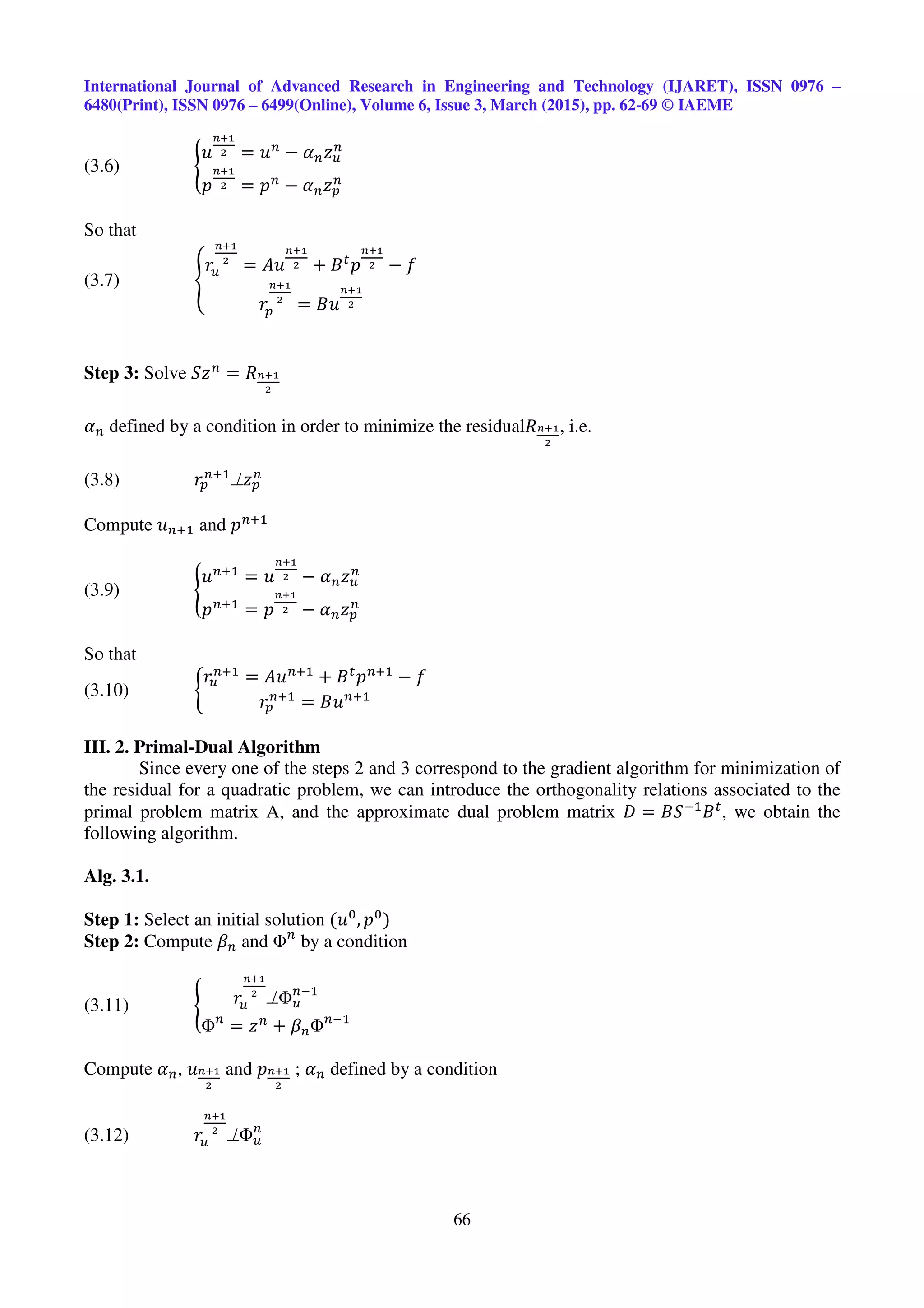
III. 1. G. “Primal-Dual” Algorithm
Step 1: Select an initial solution(ݑ
,
).
Step 2: Solve ܵݖ
= ܴ
ߙ is defined by a condition in order to minimize the residual ܴ
,
(3.5) ݎ௨
శభ
మ
= ݑ
− ߙݖ௨
Compute ݑ
శభ
మ and
శభ
మ](https://image.slidesharecdn.com/iterativemethodsforthesolutionofsaddlepointproblem-150414092958-conversion-gate01/75/Iterative-methods-for-the-solution-of-saddle-point-problem-4-2048.jpg)
![International Journal of Advanced Research in Engineering and Technology (IJARET), ISSN 0976 –
6480(Print), ISSN 0976 – 6499(Online), Volume 6, Issue 3, March (2015), pp. 62-69 © IAEME
67
(3.13) ൝
ݑ
శభ
మ = ݑ
− ߙΦ௨
శభ
మ =
− ߙݖ
So that
(3.14) ቐ
ݎ௨
శభ
మ
= ݑܣ
శభ
మ + ܤ௧
శభ
మ − ݂
ݎ
శభ
మ
= ݑܤ
శభ
మ
Step 3: Solve ܵݖ
= ܴశభ
మ
Compute ߚ and Φ
by a condition
(3.15) ݎ
ାଵ
⊥Φ
ିଵ
Φ
= ݖ
+ ߚΦିଵ
Compute ߙ, ݑାଵ, ାଵ. ߙ defined by a condition
(3.16) ݎ
ାଵ
⊥Φ
ݑାଵ
= ݑ
శభ
మ − ߙΦ௨
ାଵ
=
శభ
మ − ߙΦ
So that
ݎ௨
ାଵ
= ݑܣାଵ
+ ܤ௧
ାଵ
− ݂
ݎ
ାଵ
= ݑܤାଵ
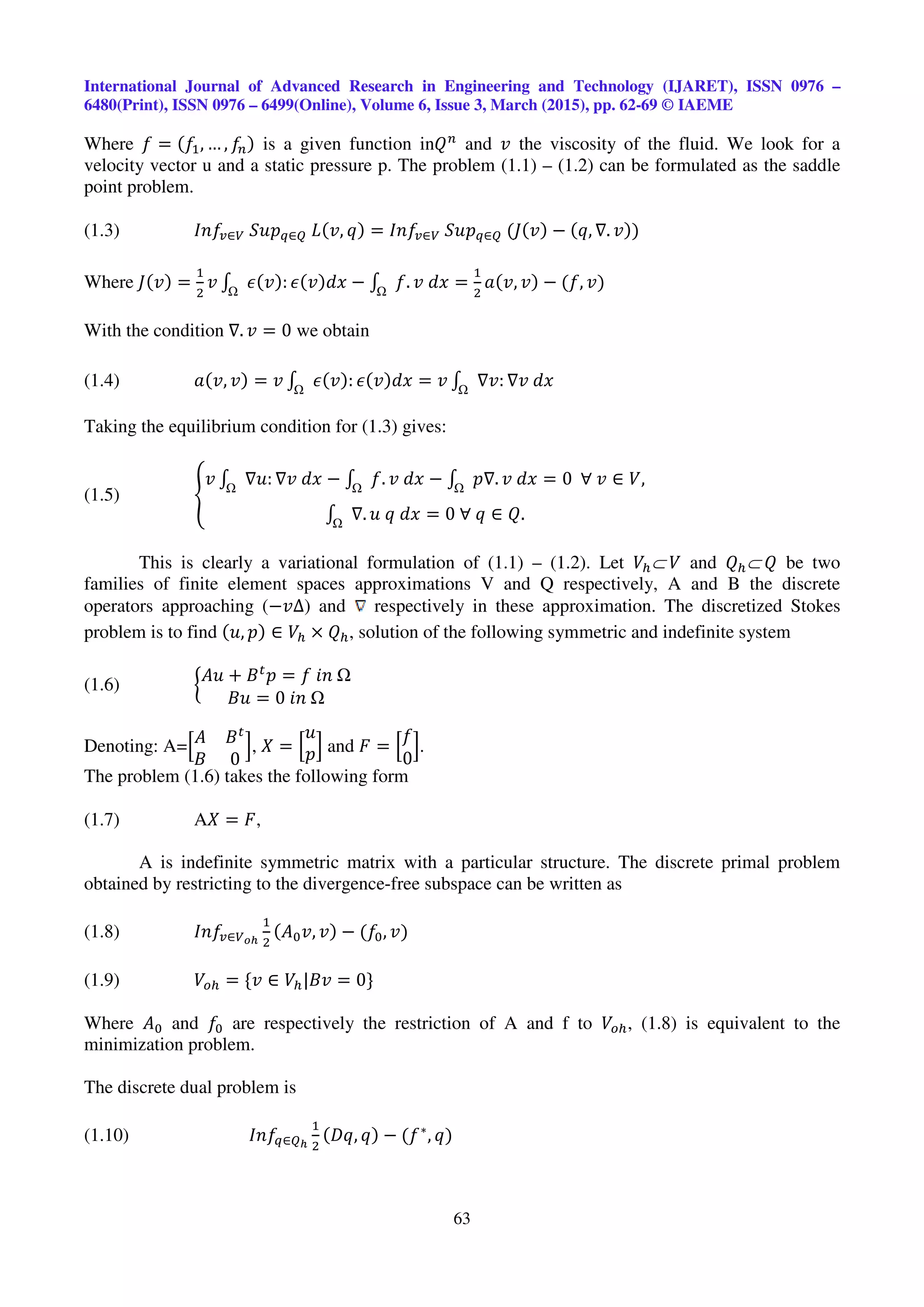
Doing some iterations of Step 2 before moving to Step 3, we obtain a convergence of the
primal variable corresponding to a minimum in v of the lagrangien ,ݒ(ܮ )ݍ and we pull back on
Uzawa’s method (Alg. 2.2).
On the contrary if we obtain convergence of the approximate dual variable and a divergence-
free solution after some iteration of Step 3, the whole process can be reduced to the primal algorithm
(Alg. 2.1). With a good preconditioner we can obtain easily the divergence-free condition and we
find once again the alg. 2.1. If the preconditioner yields rapidly the convergence of the primal
problem we find once again the Uzawa algorithm. The study of the convergence depends of the
preconditioner (cf. R. Aboulaich [1]). The convergence is illustrated in Figure 1. In the following we
present a particular example of preconditioning operator and we find a variant of Arrow-Hurwicz
algorithm.
III. 3. A Particular Case of Preconditioning
Let us denote ܵ = ቂܵ ܤ௧
0 1
ቃ , ܴ
= ቂ
ݎ௨
0
ቃ and ܴ
=
0
ݎ
൨
The G. “P-D” algorithm becomes:](https://image.slidesharecdn.com/iterativemethodsforthesolutionofsaddlepointproblem-150414092958-conversion-gate01/75/Iterative-methods-for-the-solution-of-saddle-point-problem-6-2048.jpg)

This document summarizes an iterative method for solving saddle point problems that arise in mixed finite element approximations of Stokes fluid flow problems. It presents classical solution methods like primal-dual conjugate gradient algorithms. It then proposes a general primal-dual algorithm that combines these classical methods to solve the coupled primal and dual problems simultaneously. The algorithm defines descent directions as solutions to preconditioned residual equations to minimize both the primal and dual residuals at each iteration.