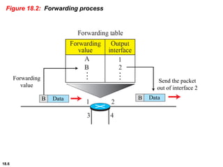
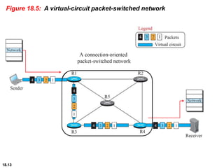
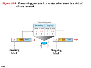
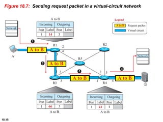
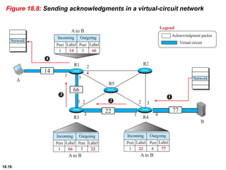
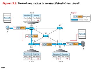
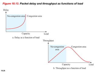
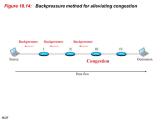
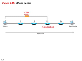
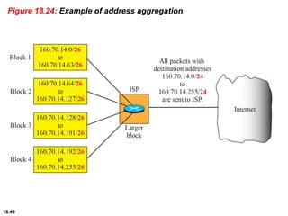
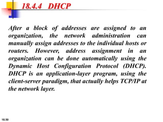
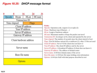
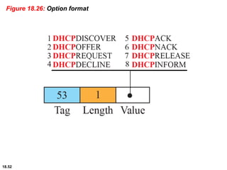
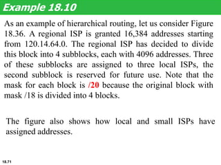
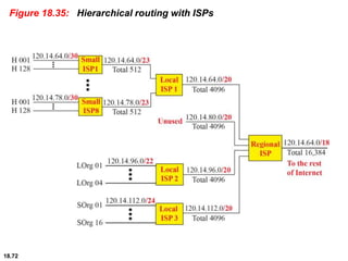
Chapter 18
Introduction
to
Network
Layer
Copyright © The McGraw-Hill Companies, Inc. Permission required for reproduction or display.
18.2
18-1 NETWORK-LAYER SERVICES
Before discussing the network layer in
the Internet today, let’s briefly discuss
the network-layer services that, in
general, are expected from a network-
layer protocol. Figure 18.1 shows the
communication between Alice and Bob
at the network layer. This is the same
scenario we used in Chapters 3 and 9 to
show the communication at the physical
and the data-link layers, respectively.
18.3
Figure 18.1: Communication at the network layer
18.4
18.18.1 Packetizing
The first duty of the network layer is definitely
packetizing: encapsulating the payload in a network-
layer packet at the source and decapsulating the
payload from the network-layer packet at the
destination. In other words, one duty of the network
layer is to carry a payload from the source to the
destination without changing it or using it. The
network layer is doing the service of a carrier such
as the postal office, which is responsible for delivery
of packages from a sender to a receiver without
changing or using the contents.
18.5
18.18.2 Routing and Forwarding
Other duties of the network layer, which are as
important as the first, are routing and forwarding,
which are directly related to each other.
18.6
Figure 18.2: Forwarding process
Forwarding
value
B Data
Send the packet
out of interface 2
B Data
18.7
18.18.3 Other Services
Let us briefly discuss other services expected from
the network layer.
18.8
18-2 PACKET SWITCHING
From the discussion of routing and
forwarding in the previous section, we
infer that a kind of switching occurs at
the network layer. A router, in fact, is a
switch that creates a connection
between an input port and an output
port (or a set of output ports), just as an
electrical switch connects the input to
the output to let electricity flow.
18.9
18.2.1 Datagram Approach
When the Internet started, to make it simple, the
network layer was designed to provide a
connectionless service in which the network-layer
protocol treats each packet independently, with each
packet having no relationship to any other packet.
The idea was that the network layer is only
responsible for delivery of packets from the source to
the destination. In this approach, the packets in a
message may or may not travel the same path to
their destination. Figure 18.3 shows the idea..
18.10
Figure 18.3: A connectionless packet-switched network
18.11
Figure 18.4: Forwarding process in a router when used in a
connectionless network
SA DA Data SA DA Data
18.12
18.2.2 Virtual-Circuit Approach
In a connection-oriented service (also called virtual-
circuit approach), there is a relationship between all
packets belonging to a message. Before all
datagrams in a message can be sent, a virtual
connection should be set up to define the path for
the datagrams. After connection setup, the
datagrams can all follow the same path. In this type
of service, not only must the packet contain the
source and destination addresses, it must also
contain a flow label, a virtual circuit identifier that
defines the virtual path the packet should follow.
18.13
Figure 18.5: A virtual-circuit packet-switched network
18.14
Figure 18.6: Forwarding process in a router when used in a virtual
circuit network
18.15
Figure 18.7: Sending request packet in a virtual-circuit network
A to B
A to B
A to B A to B
18.16
Figure 18.8: Sending acknowledgments in a virtual-circuit network
18.17
Figure 18.9: Flow of one packet in an established virtual circuit
18.18
18-3 NETWORK-LAYER PERFORMANCE
The upper-layer protocols that use the
service of the network layer expect to
receive an ideal service, but the network
layer is not perfect. The performance of
a network can be measured in terms of
delay, throughput, and packet loss.
Congestion control is an issue that can
improve the performance.
18.19
18.3.1 Delay
All of us expect instantaneous response from a
network, but a packet, from its source to its
destination, encounters delays. The delays in a
network can be divided into four types: transmission
delay, propagation delay, processing delay, and
queuing delay. Let us first discuss each of these
delay types and then show how to calculate a packet
delay from the source to the destination..
18.20
18.3.2 Throughput
Throughput at any point in a network is defined as
the number of bits passing through the point in a
second, which is actually the transmission rate of
data at that point. In a path from source to
destination, a packet may pass through several links
(networks), each with a different transmission rate.
How, then, can we determine the throughput of the
whole path? To see the situation, assume that we
have three links, each with a different transmission
rate, as shown in Figure 18.10.
18.21
Figure 18.10: Throughput in a path with three links in a series
18.22
Figure 18.11: A path through the Internet backbone
18.23
Figure 18.12: Effect of throughput in shared links
18.24
18.3.3 Packet Loss
Another issue that severely affects the performance
of communication is the number of packets lost
during transmission. When a router receives a
packet while processing another packet, the received
packet needs to be stored in the input buffer waiting
for its turn. A router, however, has an input buffer
with a limited size. A time may come when the buffer
is full and the next packet needs to be dropped. The
effect of packet loss on the Internet network layer is
that the packet needs to be resent, which in turn may
create overflow and cause more packet loss.
18.25
18.3.4 Congestion Control
Congestion control is a mechanism for improving
performance. In Chapter 23, we will discuss
congestion at the transport layer. Although
congestion at the network layer is not explicitly
addressed in the Internet model, the study of
congestion at this layer may help us to better
understand the cause of congestion at the transport
layer and find possible remedies to be used at the
network layer. Congestion at the network layer is
related to two issues, throughput and delay, which
we discussed in the previous section.
18.26
Figure 18.13. Packet delay and throughput as functions of load
18.27
Figure 18.14: Backpressure method for alleviating congestion
18.28
Figure 4.15: Choke packet
18.29
18-4 IPv4 ADDRESSES
The identifier used in the IP layer of the
TCP/IP protocol suite to identify the
connection of each device to the Internet
is called the Internet address or IP
address. An IPv4 address is a 32-bit
address that uniquely and universally
defines the connection of a host or a
router to the Internet. The IP address is
the address of the connection, not the
host or the router.
18.30
18.4.1 Address Space
A protocol like IPv4 that defines addresses has an
address space. An address space is the total number
of addresses used by the protocol. If a protocol uses
b bits to define an address, the address space is 2b
because each bit can have two different values (0 or
1). IPv4 uses 32-bit addresses, which means that the
address space is 232 or 4,294,967,296 (more than
four billion). If there were no restrictions, more than
4 billion devices could be connected to the Internet.
18.31
Figure 18.16: Three different notations in IPv4 addressing
18.32
Figure 18.17: Hierarchy in addressing
18.33
18.4.2 Classful Addressing
When the Internet started, an IPv4 address was
designed with a fixed-length prefix, but to
accommodate both small and large networks, three
fixed-length prefixes were designed instead of one (n
= 8, n = 16, and n = 24). The whole address space
was divided into five classes (class A, B, C, D, and
E), as shown in Figure 18.18. This scheme is
referred to as classful addressing. Although classful
addressing belongs to the past, it helps us to
understand classless addressing, discussed later.
18.34
Figure 18.18: Occupation of the address space in classful addressing
18.35
18.4.3 Classless Addressing
With the growth of the Internet, it was clear that a
larger address space was needed as a long-term
solution. The larger address space, however,
requires that the length of IP addresses also be
increased, which means the format of the IP packets
needs to be changed. Although the long-range
solution has already been devised and is called IPv6,
a short-term solution was also devised to use the
same address space but to change the distribution of
addresses to provide a fair share to each
organization. The short-term solution still uses IPv4
addresses, but it is called classless addressing.
18.36
Figure 18.19: Variable-length blocks in classless addressing
18.37
Figure 18.20: Slash notation (CIDR)
18.38
Figure 18.21: Information extraction in classless addressing
A classless address is given as 167.199.170.82/27. We can
find the above three pieces of information as follows. The
number of addresses in the network is 232− n = 25 = 32
addresses. The first address can be found by keeping the
first 27 bits and changing the rest of the bits to 0s.
Example 18.1
The last address can be found by keeping the first 27 bits
and changing the rest of the bits to 1s.
18.39
We repeat Example 18.1 using the mask. The mask in
dotted-decimal notation is 256.256.256.224 The AND, OR,
and NOT operations can be applied to individual bytes using
calculators and applets at the book website.
Example 18.2
18.40
In classless addressing, an address cannot per se define the
block the address belongs to. For example, the address
230.8.24.56 can belong to many blocks. Some of them are
shown below with the value of the prefix associated with
that block.
Example 18.3
18.41
18.42
Figure 18.22: Network address
An ISP has requested a block of 1000 addresses. Since 1000
is not a power of 2, 1024 addresses are granted. The prefix
length is calculated as n = 32 − log21024 = 22. An available
block, 18.14.12.0/22, is granted to the ISP. It can be seen
that the first address in decimal is 302,910,464, which is
divisible by 1024.
Example 18.4
18.43
An organization is granted a block of addresses with the
beginning address 14.24.74.0/24. The organization needs to
have 3 subblocks of addresses to use in its three subnets: one
subblock of 10 addresses, one subblock of 60 addresses, and
one subblock of 120 addresses. Design the subblocks.
Example 18.5
Solution
There are 232– 24 = 256 addresses in this block. The first
address is 14.24.74.0/24; the last address is 14.24.74.255/24.
To satisfy the third requirement, we assign addresses to
subblocks, starting with the largest and ending with the
smallest one.
18.44
a. The number of addresses in the largest subblock, which
requires 120 addresses, is not a power of 2. We allocate 128
addresses. The subnet mask for this subnet can be found as
n1 = 32 − log2 128 = 25. The first address in this block is
14.24.74.0/25; the last address is 14.24.74.127/25.
b. The number of addresses in the second largest subblock,
which requires 60 addresses, is not a power of 2 either. We
allocate 64 addresses. The subnet mask for this subnet can
be found as n2 = 32 − log2 64 = 26. The first address in this
block is 14.24.74.128/26; the last address is
14.24.74.191/26.
Example 18.5 (continued)
18.45
c. The number of addresses in the largest subblock, which
requires 10 addresses, is not a power of 2. We allocate 16
addresses. The subnet mask for this subnet can be found as
n1 = 32 − log2 16 = 28. The first address in this block is
14.24.74.192/28; the last address is 14.24.74.207/28.
Example 18.5 (continued)
If we add all addresses in the previous subblocks, the result
is 208 addresses, which means 48 addresses are left in
reserve. The first address in this range is 14.24.74.208. The
last address is 14.24.74.255. We don’t know about the prefix
length yet. Figure 18.23 shows the configuration of blocks.
We have shown the first address in each block.
18.46
18.47
Figure 18.23: Solution to Example 4.5
Figure 18.24 shows how four small blocks of addresses are
assigned to four organizations by an ISP. The ISP combines
these four blocks into one single block and advertises the
larger block to the rest of the world. Any packet destined for
this larger block should be sent to this ISP. It is the
responsibility of the ISP to forward the packet to the
appropriate organization. This is similar to routing we can
find in a postal network. All packages coming from outside
a country are sent first to the capital and then distributed to
the corresponding destination.
Example 18.6
18.48
18.49
Figure 18.24: Example of address aggregation
18.50
18.4.4 DHCP
After a block of addresses are assigned to an
organization, the network administration can
manually assign addresses to the individual hosts or
routers. However, address assignment in an
organization can be done automatically using the
Dynamic Host Configuration Protocol (DHCP).
DHCP is an application-layer program, using the
client-server paradigm, that actually helps TCP/IP at
the network layer.
18.51
Figure 18.25: DHCP message format
18.52
Figure 18.26: Option format
18.53
Figure 18.27: Operation of DHCP
18.54
Figure 18.28: FSM for the DHCP client
18.55
18.4.5 NAT
In most situations, only a portion of computers in a
small network need access to the Internet
simultaneously. A technology that can provide the
mapping between the private and universal
addresses, and at the same time support virtual
private networks, which we discuss in Chapter 32, is
Network Address Translation (NAT). The technology
allows a site to use a set of private addresses for
internal communication and a set of global Internet
addresses (at least one) for communication with the
rest of the world.
18.56
Figure 18.29: NAT
Figure 18.30: Address translation
18.57
18.58
Figure 18.31: Translation
Table 18.1: Five-column translation table
18.59
18.60
18-5 FORWARDING OF IP PACKETS
We discussed the concept of forwarding
at the network layer earlier in this
chapter. In this section, we extend the
concept to include the role of IP
addresses in forwarding. As we
discussed before, forwarding means to
place the packet in its route to its
destination.
18.61
18.5.1 Destination Address Forwarding
We first discuss forwarding based on the destination
address. This is a traditional approach, which is
prevalent today. In this case, forwarding requires a
host or a router to have a forwarding table. When a
host has a packet to send or when a router has
received a packet to be forwarded, it looks at this
table to find the next hop to deliver the packet to.
18.62
Figure 18.32: Simplified forwarding module in classless address
19.63
The first address in a block is
normally not assigned to any device;
it is used as the network address that
represents the organization
to the rest of the world.
Note
Configuration and addresses in a subnetted network
Make a forwarding table for router R1 using the
configuration in Figure 18.33.
Example 18.7
Solution
Table 18.2 shows the corresponding table.
Table 18.2: Forwarding table for router R1 in Figure 4.46
18.65
18.66
Figure 18.33: Configuration for Example 4.7
Instead of Table 18.2, we can use Table 18.3, in which the
network address/mask is given in bits.
Example 18.8
Table 18.3: Forwarding table for router R1 using prefix bits
When a packet arrives whose leftmost 26 bits in the
destination address match the bits in the first row, the packet
is sent out from interface m2. And so on.
18.67
Show the forwarding process if a packet arrives at R1 in
Figure 18.33 with the destination address 180.70.65.140.
Example 18.9
Solution
The router performs the following steps:
18. The first mask (/26) is applied to the destination address.
The result is 180.70.65.128, which does not match the
corresponding network address.
2. The second mask (/25) is applied to the destination
address. The result is 180.70.65.128, which matches the
corresponding network address. The next-hop address
and the interface number m0 are extracted for
forwarding the packet (see Chapter 5).
18.68
18.69
Figure 18.34: Address aggregation
18.70
Figure 18.35: Longest mask matching
As an example of hierarchical routing, let us consider Figure
18.36. A regional ISP is granted 16,384 addresses starting
from 120.14.64.0. The regional ISP has decided to divide
this block into 4 subblocks, each with 4096 addresses. Three
of these subblocks are assigned to three local ISPs, the
second subblock is reserved for future use. Note that the
mask for each block is /20 because the original block with
mask /18 is divided into 4 blocks.
Example 18.10
The figure also shows how local and small ISPs have
assigned addresses.
18.71
18.72
Figure 18.35: Hierarchical routing with ISPs

Intro-network layer-chapter-18_forouzan.ppt

  • 1.
    Chapter 18 Introduction to Network Layer Copyright ©The McGraw-Hill Companies, Inc. Permission required for reproduction or display.
  • 2.
    18.2 18-1 NETWORK-LAYER SERVICES Beforediscussing the network layer in the Internet today, let’s briefly discuss the network-layer services that, in general, are expected from a network- layer protocol. Figure 18.1 shows the communication between Alice and Bob at the network layer. This is the same scenario we used in Chapters 3 and 9 to show the communication at the physical and the data-link layers, respectively.
  • 3.
    18.3 Figure 18.1: Communicationat the network layer
  • 4.
    18.4 18.18.1 Packetizing The firstduty of the network layer is definitely packetizing: encapsulating the payload in a network- layer packet at the source and decapsulating the payload from the network-layer packet at the destination. In other words, one duty of the network layer is to carry a payload from the source to the destination without changing it or using it. The network layer is doing the service of a carrier such as the postal office, which is responsible for delivery of packages from a sender to a receiver without changing or using the contents.
  • 5.
    18.5 18.18.2 Routing andForwarding Other duties of the network layer, which are as important as the first, are routing and forwarding, which are directly related to each other.
  • 6.
    18.6 Figure 18.2: Forwardingprocess Forwarding value B Data Send the packet out of interface 2 B Data
  • 7.
    18.7 18.18.3 Other Services Letus briefly discuss other services expected from the network layer.
  • 8.
    18.8 18-2 PACKET SWITCHING Fromthe discussion of routing and forwarding in the previous section, we infer that a kind of switching occurs at the network layer. A router, in fact, is a switch that creates a connection between an input port and an output port (or a set of output ports), just as an electrical switch connects the input to the output to let electricity flow.
  • 9.
    18.9 18.2.1 Datagram Approach Whenthe Internet started, to make it simple, the network layer was designed to provide a connectionless service in which the network-layer protocol treats each packet independently, with each packet having no relationship to any other packet. The idea was that the network layer is only responsible for delivery of packets from the source to the destination. In this approach, the packets in a message may or may not travel the same path to their destination. Figure 18.3 shows the idea..
  • 10.
    18.10 Figure 18.3: Aconnectionless packet-switched network
  • 11.
    18.11 Figure 18.4: Forwardingprocess in a router when used in a connectionless network SA DA Data SA DA Data
  • 12.
    18.12 18.2.2 Virtual-Circuit Approach Ina connection-oriented service (also called virtual- circuit approach), there is a relationship between all packets belonging to a message. Before all datagrams in a message can be sent, a virtual connection should be set up to define the path for the datagrams. After connection setup, the datagrams can all follow the same path. In this type of service, not only must the packet contain the source and destination addresses, it must also contain a flow label, a virtual circuit identifier that defines the virtual path the packet should follow.
  • 13.
    18.13 Figure 18.5: Avirtual-circuit packet-switched network
  • 14.
    18.14 Figure 18.6: Forwardingprocess in a router when used in a virtual circuit network
  • 15.
    18.15 Figure 18.7: Sendingrequest packet in a virtual-circuit network A to B A to B A to B A to B
  • 16.
    18.16 Figure 18.8: Sendingacknowledgments in a virtual-circuit network
  • 17.
    18.17 Figure 18.9: Flowof one packet in an established virtual circuit
  • 18.
    18.18 18-3 NETWORK-LAYER PERFORMANCE Theupper-layer protocols that use the service of the network layer expect to receive an ideal service, but the network layer is not perfect. The performance of a network can be measured in terms of delay, throughput, and packet loss. Congestion control is an issue that can improve the performance.
  • 19.
    18.19 18.3.1 Delay All ofus expect instantaneous response from a network, but a packet, from its source to its destination, encounters delays. The delays in a network can be divided into four types: transmission delay, propagation delay, processing delay, and queuing delay. Let us first discuss each of these delay types and then show how to calculate a packet delay from the source to the destination..
  • 20.
    18.20 18.3.2 Throughput Throughput atany point in a network is defined as the number of bits passing through the point in a second, which is actually the transmission rate of data at that point. In a path from source to destination, a packet may pass through several links (networks), each with a different transmission rate. How, then, can we determine the throughput of the whole path? To see the situation, assume that we have three links, each with a different transmission rate, as shown in Figure 18.10.
  • 21.
    18.21 Figure 18.10: Throughputin a path with three links in a series
  • 22.
    18.22 Figure 18.11: Apath through the Internet backbone
  • 23.
    18.23 Figure 18.12: Effectof throughput in shared links
  • 24.
    18.24 18.3.3 Packet Loss Anotherissue that severely affects the performance of communication is the number of packets lost during transmission. When a router receives a packet while processing another packet, the received packet needs to be stored in the input buffer waiting for its turn. A router, however, has an input buffer with a limited size. A time may come when the buffer is full and the next packet needs to be dropped. The effect of packet loss on the Internet network layer is that the packet needs to be resent, which in turn may create overflow and cause more packet loss.
  • 25.
    18.25 18.3.4 Congestion Control Congestioncontrol is a mechanism for improving performance. In Chapter 23, we will discuss congestion at the transport layer. Although congestion at the network layer is not explicitly addressed in the Internet model, the study of congestion at this layer may help us to better understand the cause of congestion at the transport layer and find possible remedies to be used at the network layer. Congestion at the network layer is related to two issues, throughput and delay, which we discussed in the previous section.
  • 26.
    18.26 Figure 18.13. Packetdelay and throughput as functions of load
  • 27.
    18.27 Figure 18.14: Backpressuremethod for alleviating congestion
  • 28.
  • 29.
    18.29 18-4 IPv4 ADDRESSES Theidentifier used in the IP layer of the TCP/IP protocol suite to identify the connection of each device to the Internet is called the Internet address or IP address. An IPv4 address is a 32-bit address that uniquely and universally defines the connection of a host or a router to the Internet. The IP address is the address of the connection, not the host or the router.
  • 30.
    18.30 18.4.1 Address Space Aprotocol like IPv4 that defines addresses has an address space. An address space is the total number of addresses used by the protocol. If a protocol uses b bits to define an address, the address space is 2b because each bit can have two different values (0 or 1). IPv4 uses 32-bit addresses, which means that the address space is 232 or 4,294,967,296 (more than four billion). If there were no restrictions, more than 4 billion devices could be connected to the Internet.
  • 31.
    18.31 Figure 18.16: Threedifferent notations in IPv4 addressing
  • 32.
  • 33.
    18.33 18.4.2 Classful Addressing Whenthe Internet started, an IPv4 address was designed with a fixed-length prefix, but to accommodate both small and large networks, three fixed-length prefixes were designed instead of one (n = 8, n = 16, and n = 24). The whole address space was divided into five classes (class A, B, C, D, and E), as shown in Figure 18.18. This scheme is referred to as classful addressing. Although classful addressing belongs to the past, it helps us to understand classless addressing, discussed later.
  • 34.
    18.34 Figure 18.18: Occupationof the address space in classful addressing
  • 35.
    18.35 18.4.3 Classless Addressing Withthe growth of the Internet, it was clear that a larger address space was needed as a long-term solution. The larger address space, however, requires that the length of IP addresses also be increased, which means the format of the IP packets needs to be changed. Although the long-range solution has already been devised and is called IPv6, a short-term solution was also devised to use the same address space but to change the distribution of addresses to provide a fair share to each organization. The short-term solution still uses IPv4 addresses, but it is called classless addressing.
  • 36.
    18.36 Figure 18.19: Variable-lengthblocks in classless addressing
  • 37.
  • 38.
    18.38 Figure 18.21: Informationextraction in classless addressing
  • 39.
    A classless addressis given as 167.199.170.82/27. We can find the above three pieces of information as follows. The number of addresses in the network is 232− n = 25 = 32 addresses. The first address can be found by keeping the first 27 bits and changing the rest of the bits to 0s. Example 18.1 The last address can be found by keeping the first 27 bits and changing the rest of the bits to 1s. 18.39
  • 40.
    We repeat Example18.1 using the mask. The mask in dotted-decimal notation is 256.256.256.224 The AND, OR, and NOT operations can be applied to individual bytes using calculators and applets at the book website. Example 18.2 18.40
  • 41.
    In classless addressing,an address cannot per se define the block the address belongs to. For example, the address 230.8.24.56 can belong to many blocks. Some of them are shown below with the value of the prefix associated with that block. Example 18.3 18.41
  • 42.
  • 43.
    An ISP hasrequested a block of 1000 addresses. Since 1000 is not a power of 2, 1024 addresses are granted. The prefix length is calculated as n = 32 − log21024 = 22. An available block, 18.14.12.0/22, is granted to the ISP. It can be seen that the first address in decimal is 302,910,464, which is divisible by 1024. Example 18.4 18.43
  • 44.
    An organization isgranted a block of addresses with the beginning address 14.24.74.0/24. The organization needs to have 3 subblocks of addresses to use in its three subnets: one subblock of 10 addresses, one subblock of 60 addresses, and one subblock of 120 addresses. Design the subblocks. Example 18.5 Solution There are 232– 24 = 256 addresses in this block. The first address is 14.24.74.0/24; the last address is 14.24.74.255/24. To satisfy the third requirement, we assign addresses to subblocks, starting with the largest and ending with the smallest one. 18.44
  • 45.
    a. The numberof addresses in the largest subblock, which requires 120 addresses, is not a power of 2. We allocate 128 addresses. The subnet mask for this subnet can be found as n1 = 32 − log2 128 = 25. The first address in this block is 14.24.74.0/25; the last address is 14.24.74.127/25. b. The number of addresses in the second largest subblock, which requires 60 addresses, is not a power of 2 either. We allocate 64 addresses. The subnet mask for this subnet can be found as n2 = 32 − log2 64 = 26. The first address in this block is 14.24.74.128/26; the last address is 14.24.74.191/26. Example 18.5 (continued) 18.45
  • 46.
    c. The numberof addresses in the largest subblock, which requires 10 addresses, is not a power of 2. We allocate 16 addresses. The subnet mask for this subnet can be found as n1 = 32 − log2 16 = 28. The first address in this block is 14.24.74.192/28; the last address is 14.24.74.207/28. Example 18.5 (continued) If we add all addresses in the previous subblocks, the result is 208 addresses, which means 48 addresses are left in reserve. The first address in this range is 14.24.74.208. The last address is 14.24.74.255. We don’t know about the prefix length yet. Figure 18.23 shows the configuration of blocks. We have shown the first address in each block. 18.46
  • 47.
  • 48.
    Figure 18.24 showshow four small blocks of addresses are assigned to four organizations by an ISP. The ISP combines these four blocks into one single block and advertises the larger block to the rest of the world. Any packet destined for this larger block should be sent to this ISP. It is the responsibility of the ISP to forward the packet to the appropriate organization. This is similar to routing we can find in a postal network. All packages coming from outside a country are sent first to the capital and then distributed to the corresponding destination. Example 18.6 18.48
  • 49.
    18.49 Figure 18.24: Exampleof address aggregation
  • 50.
    18.50 18.4.4 DHCP After ablock of addresses are assigned to an organization, the network administration can manually assign addresses to the individual hosts or routers. However, address assignment in an organization can be done automatically using the Dynamic Host Configuration Protocol (DHCP). DHCP is an application-layer program, using the client-server paradigm, that actually helps TCP/IP at the network layer.
  • 51.
  • 52.
  • 53.
  • 54.
    18.54 Figure 18.28: FSMfor the DHCP client
  • 55.
    18.55 18.4.5 NAT In mostsituations, only a portion of computers in a small network need access to the Internet simultaneously. A technology that can provide the mapping between the private and universal addresses, and at the same time support virtual private networks, which we discuss in Chapter 32, is Network Address Translation (NAT). The technology allows a site to use a set of private addresses for internal communication and a set of global Internet addresses (at least one) for communication with the rest of the world.
  • 56.
  • 57.
    Figure 18.30: Addresstranslation 18.57
  • 58.
  • 59.
    Table 18.1: Five-columntranslation table 18.59
  • 60.
    18.60 18-5 FORWARDING OFIP PACKETS We discussed the concept of forwarding at the network layer earlier in this chapter. In this section, we extend the concept to include the role of IP addresses in forwarding. As we discussed before, forwarding means to place the packet in its route to its destination.
  • 61.
    18.61 18.5.1 Destination AddressForwarding We first discuss forwarding based on the destination address. This is a traditional approach, which is prevalent today. In this case, forwarding requires a host or a router to have a forwarding table. When a host has a packet to send or when a router has received a packet to be forwarded, it looks at this table to find the next hop to deliver the packet to.
  • 62.
    18.62 Figure 18.32: Simplifiedforwarding module in classless address
  • 63.
    19.63 The first addressin a block is normally not assigned to any device; it is used as the network address that represents the organization to the rest of the world. Note
  • 64.
    Configuration and addressesin a subnetted network
  • 65.
    Make a forwardingtable for router R1 using the configuration in Figure 18.33. Example 18.7 Solution Table 18.2 shows the corresponding table. Table 18.2: Forwarding table for router R1 in Figure 4.46 18.65
  • 66.
  • 67.
    Instead of Table18.2, we can use Table 18.3, in which the network address/mask is given in bits. Example 18.8 Table 18.3: Forwarding table for router R1 using prefix bits When a packet arrives whose leftmost 26 bits in the destination address match the bits in the first row, the packet is sent out from interface m2. And so on. 18.67
  • 68.
    Show the forwardingprocess if a packet arrives at R1 in Figure 18.33 with the destination address 180.70.65.140. Example 18.9 Solution The router performs the following steps: 18. The first mask (/26) is applied to the destination address. The result is 180.70.65.128, which does not match the corresponding network address. 2. The second mask (/25) is applied to the destination address. The result is 180.70.65.128, which matches the corresponding network address. The next-hop address and the interface number m0 are extracted for forwarding the packet (see Chapter 5). 18.68
  • 69.
  • 70.
  • 71.
    As an exampleof hierarchical routing, let us consider Figure 18.36. A regional ISP is granted 16,384 addresses starting from 120.14.64.0. The regional ISP has decided to divide this block into 4 subblocks, each with 4096 addresses. Three of these subblocks are assigned to three local ISPs, the second subblock is reserved for future use. Note that the mask for each block is /20 because the original block with mask /18 is divided into 4 blocks. Example 18.10 The figure also shows how local and small ISPs have assigned addresses. 18.71
  • 72.