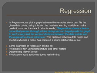
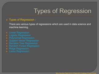
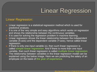
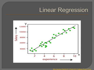
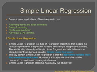
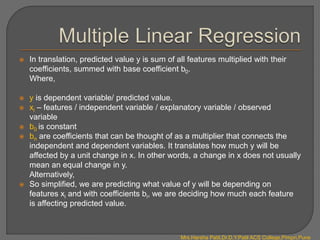
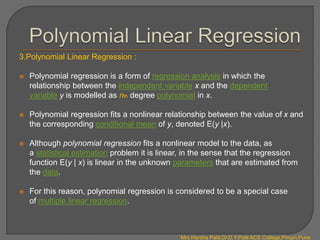
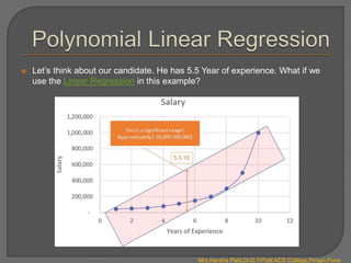
The document discusses regression analysis and different types of regression models. It defines regression analysis as a statistical method to model the relationship between a dependent variable and one or more independent variables. It explains linear regression, multiple linear regression, and polynomial regression. Linear regression finds the linear relationship between two variables, multiple linear regression handles multiple independent variables, and polynomial regression models nonlinear relationships using polynomial functions. Examples and code snippets in Python are provided to illustrate simple and multiple linear regression analysis.


![ Simple Linear Regression in Python :
#importing libraries
import numpy as np
import matplotlib.pyplot as plt
import pandas as pd
# Importing the dataset
dataset = pd.read_csv('salary_data.csv')
x = dataset.iloc[:, :-1].values
y = dataset.iloc[:, 1].values
Mrs.Harsha Patil,Dr.D.Y.Patil ACS College,Pimpri,Pune](https://image.slidesharecdn.com/introductiontoregression-240407070742-98e1c698/85/Introduction-to-Regression-pptx-13-320.jpg)


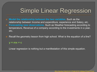
![ One plot is from training set and another from test. Blue lines are in the
same direction. Our model is good to use now.
Now we can use it to calculate (predict) any values of X depends on y or any
values of y depends on X. This can be done by using predict() function as
follows:
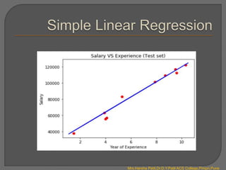
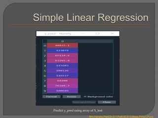
# Predicting the result of 5 Years Experience
y_pred =regressor.predict(np.array([5]).reshape(1, 1))
Output :
The value of y_pred with X = 5 (5 Years Experience) is 73545.90
You can offer to your candidate the salary of ₹ 73,545.90
and this is the best salary for him!
Mrs.Harsha Patil,Dr.D.Y.Patil ACS College,Pimpri,Pune](https://image.slidesharecdn.com/introductiontoregression-240407070742-98e1c698/85/Introduction-to-Regression-pptx-18-320.jpg)


![Multiple Linear Regression in Python :
#Importing libraries
import numpy as np
import matplotlib.pyplot as plt
import pandas as pd
from sklearn.model_selection import train_test_split
from sklearn.linear_model import LinearRegression
# Importing the dataset
dataset = pd.read_csv('salary_data.csv')
x = dataset.iloc[:, :-1].values
y = dataset.iloc[:, 4].values
#Splitting the dataset into the Training set and Test set
X_train, X_test, y_train, y_test = train_test_split(X, Y, test_size = 0.2,
random_state = 0)
Mrs.Harsha Patil,Dr.D.Y.Patil ACS College,Pimpri,Pune](https://image.slidesharecdn.com/introductiontoregression-240407070742-98e1c698/85/Introduction-to-Regression-pptx-24-320.jpg)
![# Fitting Multiple Linear Regression to the Training set.
regressor = LinearRegression()
regressor.fit(X_train, y_train)
Now! We have the Multiple Linear Regression model, we can use it to
calculate (predict) any values of x depends on y or any values of y depends
on x. This is how we do it as follows:
‘’’Predicting the result of salary of new employee with 5 Years of total
Experience, 2 years as team lead Experience, one year as project manager
and has 2 certifications’’’
x_new = [[5],[2],[1],[2]]
y_pred = regressor.predict(np.array(x_new).reshape(1, 4))
print(y_pred)
accuracy = (regressor.score(X_test,y_test))
print(accuracy)
Mrs.Harsha Patil,Dr.D.Y.Patil ACS College,Pimpri,Pune](https://image.slidesharecdn.com/introductiontoregression-240407070742-98e1c698/85/Introduction-to-Regression-pptx-25-320.jpg)
![Output :
The value of y_pred with x_new = [[5],[2],[1],[2]](5 Years of total Experience,
2 years as team lead, one year as project manager and 2 Certifications) is ₹
48017.20
You can offer to your candidate the salary of ₹48017.20 and this is the
best salary for him!
Mrs.Harsha Patil,Dr.D.Y.Patil ACS College,Pimpri,Pune](https://image.slidesharecdn.com/introductiontoregression-240407070742-98e1c698/85/Introduction-to-Regression-pptx-26-320.jpg)


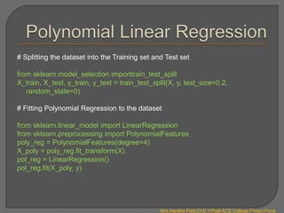
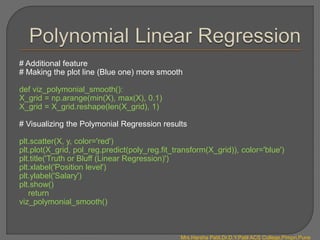
![Polynomial Linear Regression in Python :
#Importing libraries
import numpy as np
import matplotlib.pyplot as plt
import pandas as pd
# Importing the dataset
dataset = pd.read_csv(‘position_salaries’)
X = dataset.iloc[:, 1:2].values
y = dataset.iloc[:, 2].values
Mrs.Harsha Patil,Dr.D.Y.Patil ACS College,Pimpri,Pune](https://image.slidesharecdn.com/introductiontoregression-240407070742-98e1c698/85/Introduction-to-Regression-pptx-32-320.jpg)


![Last step, let’s predict the value of our candidate (with 5.5 YE) Polynomial
Regression model:
# Predicting a new result with Polymonial Regression
print(pol_reg.predict(poly_reg.fit_transform([[5.5]])))
Output:
It’s time to let our candidate know, we will offer him a best salary in class with₹
132,148!
Mrs.Harsha Patil,Dr.D.Y.Patil ACS College,Pimpri,Pune](https://image.slidesharecdn.com/introductiontoregression-240407070742-98e1c698/85/Introduction-to-Regression-pptx-37-320.jpg)


![[系列活動] 一日搞懂生成式對抗網路](https://cdn.slidesharecdn.com/ss_thumbnails/gan-170813004356-thumbnail.jpg?width=640&height=640&fit=bounds)


![[DSC Europe 25] Elena Menshikova - AI-Powered Operational Excellence: Revolut...](https://cdn.slidesharecdn.com/ss_thumbnails/es6nholbqy3zaao2c2yd-2-elena-menshikova-data-ai-in-decision-making-260115093812-4fba8b38-thumbnail.jpg?width=640&height=640&fit=bounds)


![[DSC Europe 25] Mijat Kustudic - Building Financial Intelligence with AI Agen...](https://cdn.slidesharecdn.com/ss_thumbnails/38y2lb5lse6wstegtvas-3-mijat-kustudic-building-financial-intelligence-with-ai-agents-260114111931-1a4783ce-thumbnail.jpg?width=640&height=640&fit=bounds)

![[DSC Europe 25] Ivica Milaric - The Future of Gaming and AI Tools.pptx](https://cdn.slidesharecdn.com/ss_thumbnails/tijgzsmgse2kj2y5pzzp-5-ivica-milaric-the-future-of-gaming-x-ai-tools-260114111931-87c2b3ac-thumbnail.jpg?width=640&height=640&fit=bounds)


