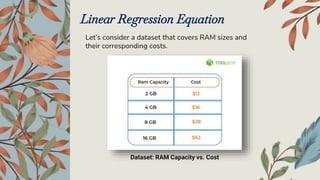
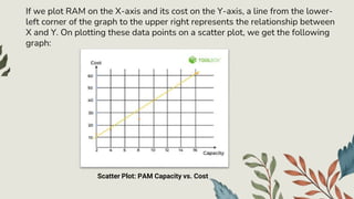
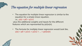
Regression via
Mathematical
Functions
Linear Regression
 Linear regression is defined as an algorithm that provides a
linear relationship between an independent variable and a
dependent variable to predict the outcome of future events.
 It is a statistical method used in data science and machine
learning for predictive analysis.
 The regression model predicts the value of the dependent
variable, which is the response or outcome variable being
analyzed or studied.
 Linear regression is a supervised learning algorithm that
simulates a mathematical relationship between variables and
makes predictions for continuous or numeric variables such as
sales, salary, age, product price, etc.
 This analysis method is advantageous when at least two
variables are available in the data, as observed in stock market
forecasting, portfolio management, scientific analysis, etc.
 A sloped straight line represents the linear regression model.
Applications of Linear Regression
In the figure,
 X-axis = Independent variable
 Y-axis = Output / dependent variable
Line of regression = Best fit line for a model
• Here, a line is plotted for the given
data points that suitably fit all the
issues.
• Hence, it is called the ‘best fit
line.’
• The goal of the linear regression
algorithm is to find this best fit line
seen in the figure.
Key benefits of linear regression
1. Easy implementation
The linear regression model is computationally simple to implement as it does not
demand a lot of engineering overheads, neither before the model launch nor during its
maintenance.
2. Interpretability
Unlike other deep learning models (neural networks), linear regression is relatively
straightforward. As a result, this algorithm stands ahead of black-box models that fall
short in justifying which input variable causes the output variable to change.
3. Scalability
Linear regression is not computationally heavy and, therefore, fits well in cases where
scaling is essential. For example, the model can scale well regarding increased data
volume (big data).
4. Optimal for online settings
The ease of computation of these algorithms allows them to be used in online settings.
The model can be trained and retrained with each new example to generate predictions
in real-time.
Linear Regression Equation
Let’s consider a dataset that covers RAM sizes and
their corresponding costs.
Dataset: RAM Capacity vs. Cost
If we plot RAM on the X-axis and its cost on the Y-axis, a line from the lower-
left corner of the graph to the upper right represents the relationship between
X and Y. On plotting these data points on a scatter plot, we get the following
graph:
Scatter Plot: PAM Capacity vs. Cost
• The regression model defines a linear function between the X and Y
variables that best showcases the relationship between the two.
• It is represented by the slant line seen in the above figure, where the
objective is to determine an optimal ‘regression line’ that best fits all
the individual data points.
Mathematically these slant lines follow the following equation,
Y = m*X + b
Where X = dependent variable (target)
Y = independent variable
m = slope of the line (slope is defined as the ‘rise’ over the ‘run’)
However, machine learning experts have a different notation to the above
slope-line equation,
y(x) = p0 + p1 * x
where,
•y = output variable. Variable y represents the continuous value that the model
tries to predict.
•x = input variable. In machine learning, x is the feature, while it is termed the
independent variable in statistics. Variable x represents the input information
provided to the model at any given time.
•p0 = y-axis intercept (or the bias term).
•p1 = the regression coefficient or scale factor. In classical statistics, p1 is the
equivalent of the slope of the best-fit straight line of the linear regression
model.
•pi = weights (in general).
Thus, regression modeling is all about finding the values for the unknown
parameters of the equation, i.e., values for p0 and p1 (weights).
The equation for multiple linear regression
• The equation for multiple linear regression is similar to the
equation for a simple linear equation,
i.e., y(x) = p0 + p1x1
-plus the additional weights and inputs for the different
features which are represented by p(n)x(n).
• The formula for multiple linear regression would look like,
y(x) = p0 + p1x1 + p2x2 + … + p(n)x(n)
PYTHON CODE FOR OBTAINING THE LINEAR REGRESSION RAM CAPACITY VS COST DATASET:
import numpy as np
from sklearn.linear_model import LinearRegression
import matplotlib.pyplot as plt
# Get the data from the image
ram_capacity = np.array([2, 4, 8, 16])
ram_cost = np.array([12, 16, 28, 62])
# Create a linear regression model
model = LinearRegression()
# Fit the model to the data
model.fit(ram_capacity[:, np.newaxis], ram_cost)
# Get the slope and intercept of the regression line
slope = model.coef_[0][0] intercept = model.intercept_[0]
# Generate the regression line
ram_reg = np.linspace(min(ram_capacity), max(ram_capacity), 100)
cost_reg = slope * ram_reg + intercept
# Plot the data and the regression line
plt.scatter(ram_capacity, ram_cost)
plt.plot(ram_reg, cost_reg, color='red’)
plt.xlabel('Capacity’)
plt.ylabel('Cost’)
plt.title('Linear Regression of RAM Cost vs. RAM Capacity’)
plt.show()
CREDITS: This presentation template was created by
Slidesgo, and includes icons by Flaticon, and
infographics & images by Freepik
OUTPUT:

linear regression in machine learning.pptx

  • 1.
  • 2.
    Linear Regression  Linearregression is defined as an algorithm that provides a linear relationship between an independent variable and a dependent variable to predict the outcome of future events.  It is a statistical method used in data science and machine learning for predictive analysis.  The regression model predicts the value of the dependent variable, which is the response or outcome variable being analyzed or studied.
  • 3.
     Linear regressionis a supervised learning algorithm that simulates a mathematical relationship between variables and makes predictions for continuous or numeric variables such as sales, salary, age, product price, etc.  This analysis method is advantageous when at least two variables are available in the data, as observed in stock market forecasting, portfolio management, scientific analysis, etc.  A sloped straight line represents the linear regression model. Applications of Linear Regression
  • 4.
    In the figure, X-axis = Independent variable  Y-axis = Output / dependent variable Line of regression = Best fit line for a model • Here, a line is plotted for the given data points that suitably fit all the issues. • Hence, it is called the ‘best fit line.’ • The goal of the linear regression algorithm is to find this best fit line seen in the figure.
  • 5.
    Key benefits oflinear regression 1. Easy implementation The linear regression model is computationally simple to implement as it does not demand a lot of engineering overheads, neither before the model launch nor during its maintenance. 2. Interpretability Unlike other deep learning models (neural networks), linear regression is relatively straightforward. As a result, this algorithm stands ahead of black-box models that fall short in justifying which input variable causes the output variable to change. 3. Scalability Linear regression is not computationally heavy and, therefore, fits well in cases where scaling is essential. For example, the model can scale well regarding increased data volume (big data). 4. Optimal for online settings The ease of computation of these algorithms allows them to be used in online settings. The model can be trained and retrained with each new example to generate predictions in real-time.
  • 6.
    Linear Regression Equation Let’sconsider a dataset that covers RAM sizes and their corresponding costs. Dataset: RAM Capacity vs. Cost
  • 7.
    If we plotRAM on the X-axis and its cost on the Y-axis, a line from the lower- left corner of the graph to the upper right represents the relationship between X and Y. On plotting these data points on a scatter plot, we get the following graph: Scatter Plot: PAM Capacity vs. Cost
  • 8.
    • The regressionmodel defines a linear function between the X and Y variables that best showcases the relationship between the two. • It is represented by the slant line seen in the above figure, where the objective is to determine an optimal ‘regression line’ that best fits all the individual data points. Mathematically these slant lines follow the following equation, Y = m*X + b Where X = dependent variable (target) Y = independent variable m = slope of the line (slope is defined as the ‘rise’ over the ‘run’)
  • 9.
    However, machine learningexperts have a different notation to the above slope-line equation, y(x) = p0 + p1 * x where, •y = output variable. Variable y represents the continuous value that the model tries to predict. •x = input variable. In machine learning, x is the feature, while it is termed the independent variable in statistics. Variable x represents the input information provided to the model at any given time. •p0 = y-axis intercept (or the bias term). •p1 = the regression coefficient or scale factor. In classical statistics, p1 is the equivalent of the slope of the best-fit straight line of the linear regression model. •pi = weights (in general). Thus, regression modeling is all about finding the values for the unknown parameters of the equation, i.e., values for p0 and p1 (weights).
  • 10.
    The equation formultiple linear regression • The equation for multiple linear regression is similar to the equation for a simple linear equation, i.e., y(x) = p0 + p1x1 -plus the additional weights and inputs for the different features which are represented by p(n)x(n). • The formula for multiple linear regression would look like, y(x) = p0 + p1x1 + p2x2 + … + p(n)x(n)
  • 11.
    PYTHON CODE FOROBTAINING THE LINEAR REGRESSION RAM CAPACITY VS COST DATASET: import numpy as np from sklearn.linear_model import LinearRegression import matplotlib.pyplot as plt # Get the data from the image ram_capacity = np.array([2, 4, 8, 16]) ram_cost = np.array([12, 16, 28, 62]) # Create a linear regression model model = LinearRegression() # Fit the model to the data model.fit(ram_capacity[:, np.newaxis], ram_cost) # Get the slope and intercept of the regression line slope = model.coef_[0][0] intercept = model.intercept_[0] # Generate the regression line ram_reg = np.linspace(min(ram_capacity), max(ram_capacity), 100) cost_reg = slope * ram_reg + intercept # Plot the data and the regression line plt.scatter(ram_capacity, ram_cost) plt.plot(ram_reg, cost_reg, color='red’) plt.xlabel('Capacity’) plt.ylabel('Cost’) plt.title('Linear Regression of RAM Cost vs. RAM Capacity’) plt.show()
  • 12.
    CREDITS: This presentationtemplate was created by Slidesgo, and includes icons by Flaticon, and infographics & images by Freepik OUTPUT: