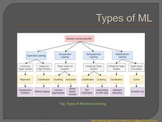
There are four main types of machine learning:
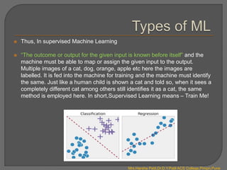
1. Supervised learning uses labelled data to map inputs to outputs. It includes classification and regression.
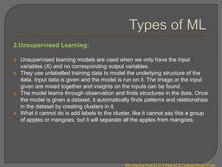
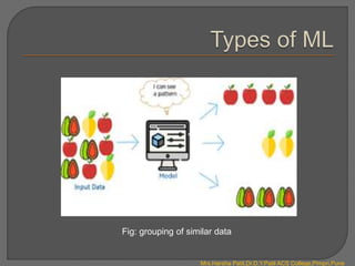
2. Unsupervised learning uses unlabeled data to find hidden patterns in data by clustering them. It includes association and clustering.
3. Semi-supervised learning uses a combination of labelled and unlabeled data.
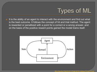
4. Reinforcement learning involves an agent learning through trial-and-error interactions with an environment. The agent receives rewards or penalties to maximize rewards.