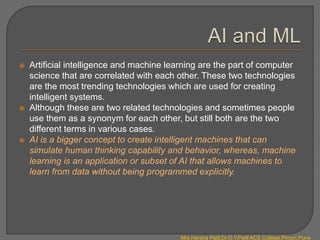
The document discusses various aspects of machine learning including:
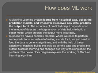
- Machine learning involves extracting knowledge from data to enable machines to learn without being explicitly programmed. It uses algorithms to model data and make predictions.
- The machine learning process includes data acquisition, processing, modeling, execution, and deployment. Algorithms are used to model the data and refine solutions.
- Machine learning has applications in healthcare, finance, retail, travel, and media by providing personalized recommendations, detecting fraud, optimizing prices and improving customer service.
- Data preprocessing is required to clean and transform raw data before training machine learning models. This includes data integration, cleaning, and transformation techniques.


![Example: We have registered the speed of 13 cars:
speed = [99,86,87,88,111,86,103,87,94,78,77,85,86]
1.Mean -The average value.
(99+86+87+88+111+86+103+87+94+78+77+85+86) / 13 = 89.77
The NumPy module has NumPy mean() method for this.
import numpy
speed = [99,86,87,88,111,86,103,87,94,78,77,85,86]
x = numpy.mean(speed)
print(x)
Mrs.Harsha Patil,Dr.D.Y.Patil ACS College,Pimpri,Pune](https://image.slidesharecdn.com/introductiontomachinelearning-240407070418-c2dd6b41/85/Introduction-to-Machine-Learning-pptx-37-320.jpg)
![2.Median - The midpoint value.
The median value is the value in the middle, after you have sorted all the
values:
(77, 78, 85, 86, 86, 86, 87, 87, 88, 94, 99, 103, 111)
It is important that the numbers are sorted before you can find the median
The NumPy module has a NumPy median() method to find the middle value.
import numpy
speed = [99,86,87,88,111,86,103,87,94,78,77,85,86]
x = numpy. median(speed)
print(x)
If there are two numbers in the middle, divide the sum of those numbers by
two.
Ex. (77, 78, 85, 86, 86, 86, 87, 87, 94, 98, 99, 103)
(86 + 87) / 2 = 86.5
Mrs.Harsha Patil,Dr.D.Y.Patil ACS College,Pimpri,Pune](https://image.slidesharecdn.com/introductiontomachinelearning-240407070418-c2dd6b41/85/Introduction-to-Machine-Learning-pptx-38-320.jpg)
![3.Mode - The most common value.
The Mode value is the value that appears the most number of times.
(99, 86, 87, 88, 111, 86, 103, 87, 94, 78, 77, 85, 86) = 86
The SciPy module has a SciPy mode() method to find the number
that appears the most.
from scipy import stats
speed = [99,86,87,88,111,86,103,87,94,78,77,85,86]
x = stats. mode(speed)
print(x)
Mrs.Harsha Patil,Dr.D.Y.Patil ACS College,Pimpri,Pune](https://image.slidesharecdn.com/introductiontomachinelearning-240407070418-c2dd6b41/85/Introduction-to-Machine-Learning-pptx-39-320.jpg)
![ Standard deviation is a number that describes how spread out the values
are.
A low standard deviation means that most of the numbers are close to the
mean (average) value.
A high standard deviation means that the values are spread out over a wider
range.
Example: We have registered the speed of 7 cars:
speed = [86,87,88,86,87,85,86]
The standard deviation is:0.9
Meaning that most of the values are within the range of 0.9 from the mean
value, which is 86.4.
Example: We have registered the speed of another 7 cars:
speed = [32,111,138,28,59,77,97]
The standard deviation is:37.85
Meaning that most of the values are within the range of 37.85 from the
mean value, which is 77.4.
A higher standard deviation indicates that the values are spread out
over a wider range.
Mrs.Harsha Patil,Dr.D.Y.Patil ACS College,Pimpri,Pune](https://image.slidesharecdn.com/introductiontomachinelearning-240407070418-c2dd6b41/85/Introduction-to-Machine-Learning-pptx-40-320.jpg)
![ The NumPy module has a NumPy std() method to find the standard
deviation.
import numpy
speed = [86,87,88,86,87,85,86]
x = numpy.std(speed)
print(x)
import numpy
speed = [32,111,138,28,59,77,97]
x = numpy.std(speed)
print(x)
Standard Deviation is often represented by the symbol Sigma: σ
Mrs.Harsha Patil,Dr.D.Y.Patil ACS College,Pimpri,Pune](https://image.slidesharecdn.com/introductiontomachinelearning-240407070418-c2dd6b41/85/Introduction-to-Machine-Learning-pptx-41-320.jpg)

![3. For each difference: find the square value:
(-45.4)2 = 2061.16
(33.6)2 = 1128.96
(60.6)2 = 3672.36
(-49.4)2 = 2440.36
(-18.4)2 = 338.56
(- 0.4)2 = 0.16
(19.6)2 = 384.16
4. The variance is the average number of these squared differences:
(2061.16+1128.96+3672.36+2440.36+338.56+0.16+384.16) / 7 = 1432.6
The NumPy module has a NumPy var() method to find the variance.
import numpy
speed = [32,111,138,28,59,77,97]
x = numpy.var(speed)
print(x)
Variance is often represented by the symbol Sigma Square: σ2
Mrs.Harsha Patil,Dr.D.Y.Patil ACS College,Pimpri,Pune](https://image.slidesharecdn.com/introductiontomachinelearning-240407070418-c2dd6b41/85/Introduction-to-Machine-Learning-pptx-43-320.jpg)
![ Percentiles are used in statistics to give you a number that describes the
value that a given percent of the values are lower than.
Example: we have an array of the ages of all the people that lives in a street.
ages = [5,31,43,48,50,41,7,11,15,39,80,82,32,2,8,6,25,36,27,61,31]
What is the 75. percentile? The answer is 43, meaning that 75% of the people
are 43 or younger.
The NumPy module has a method NumPy percentile() to find the percentiles:
import numpy
ages = [5,31,43,48,50,41,7,11,15,39,80,82,32,2,8,6,25,36,27,61,31]
x = numpy.percentile(ages, 75)
print(x)
What is the age that 90% of the people are younger than?
import numpy
ages = [5,31,43,48,50,41,7,11,15,39,80,82,32,2,8,6,25,36,27,61,31]
x = numpy.percentile(ages, 90)
print(x)
Mrs.Harsha Patil,Dr.D.Y.Patil ACS College,Pimpri,Pune](https://image.slidesharecdn.com/introductiontomachinelearning-240407070418-c2dd6b41/85/Introduction-to-Machine-Learning-pptx-44-320.jpg)


![ The Matplotlib module has a method for drawing scatter plots, it needs two
arrays of the same length, one for the values of the x-axis, and one for the
values of the y-axis:
x = [5,7,8,7,2,17,2,9,4,11,12,9,6]
y = [99,86,87,88,111,86,103,87,94,78,77,85,86]
The x array represents the age of each car.
The y array represents the speed of each car.
Example
Use the scatter() method to draw a scatter plot diagram:
import matplotlib.pyplot as plt
x = [5,7,8,7,2,17,2,9,4,11,12,9,6]
y = [99,86,87,88,111,86,103,87,94,78,77,85,86]
plt.scatter(x, y)
plt.show()
Mrs.Harsha Patil,Dr.D.Y.Patil ACS College,Pimpri,Pune](https://image.slidesharecdn.com/introductiontomachinelearning-240407070418-c2dd6b41/85/Introduction-to-Machine-Learning-pptx-78-320.jpg)


![ By pressing raw button in the link, copy this dataset and store it in Data.csv
file, in the folder where your program is stored.
In order to import this dataset into our script, we are apparently going to use
pandas as follows.
dataset = pd.read_csv('Data.csv') # to import the dataset into a variable
# Splitting the attributes into independent and dependent attributes
X = dataset.iloc[:, :-1].values # attributes to determine independent variable /
Class
Y = dataset.iloc[:, -1].values # dependent variable / Class
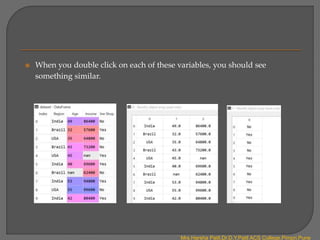
When you run this code section, along with libraries, you should not see any
errors. When successfully executed, you can move to variable explorer in the
Spyder UI and you will see the following three variables.
Mrs.Harsha Patil,Dr.D.Y.Patil ACS College,Pimpri,Pune](https://image.slidesharecdn.com/introductiontomachinelearning-240407070418-c2dd6b41/85/Introduction-to-Machine-Learning-pptx-86-320.jpg)


![# handling the missing data and replace missing values with nan from
numpy and replace with mean of all the other values
imputer = SimpleImputer(missing_values=np.nan, strategy='mean’)
imputer = imputer.fit(X[:, 1:])
X[:, 1:] = imputer.transform(X[:, 1:])
After execution of this code, the independent variable X will transform
into the following.
Mrs.Harsha Patil,Dr.D.Y.Patil ACS College,Pimpri,Pune](https://image.slidesharecdn.com/introductiontomachinelearning-240407070418-c2dd6b41/85/Introduction-to-Machine-Learning-pptx-90-320.jpg)

![ # encode categorical data
from sklearn.preprocessing import LabelEncoder, OneHotEncoder
labelencoder_X = LabelEncoder()
X[:, 0] = labelencoder_X.fit_transform(X[:, 0])
rg = ColumnTransformer([("Region", OneHotEncoder(), [0])], remainder =
'passthrough’)
X = rg.fit_transform(X)
labelencoder_Y = LabelEncoder()
Y = labelencoder_Y.fit_transform(Y)
After execution of this code, the independent variable X and dependent
variable Y will transform into the following.
Mrs.Harsha Patil,Dr.D.Y.Patil ACS College,Pimpri,Pune](https://image.slidesharecdn.com/introductiontomachinelearning-240407070418-c2dd6b41/85/Introduction-to-Machine-Learning-pptx-93-320.jpg)


![[DSC Europe 25] Elena Menshikova - AI-Powered Operational Excellence: Revolut...](https://cdn.slidesharecdn.com/ss_thumbnails/es6nholbqy3zaao2c2yd-2-elena-menshikova-data-ai-in-decision-making-260115093812-4fba8b38-thumbnail.jpg?width=640&height=640&fit=bounds)
![[DSC Europe 25] Danilo Djukanovic - From Vibes to KPIs: Turning Culture Into ...](https://cdn.slidesharecdn.com/ss_thumbnails/inqestws5wf0cik2glgv-3-danilo-djukanovic-from-vibes-to-kpis-presentation-260114111931-dacff81f-thumbnail.jpg?width=640&height=640&fit=bounds)

![[DSC Europe 25] Srba Markovic - From Pilot to Production: Overcoming AI Deplo...](https://cdn.slidesharecdn.com/ss_thumbnails/yjjmrtytmwbalxlba7px-4-srba-markovic-from-pilot-to-production-overcoming-ai-deployment-blockers-with-260114111931-4a892d44-thumbnail.jpg?width=640&height=640&fit=bounds)


![[DSC Europe 25] Dragan Jerosimovic - The Anatomy of a Narrative Simulation.pdf](https://cdn.slidesharecdn.com/ss_thumbnails/vzputuprdqr6zwbrwdcw-1-dragan-jerosimovic-the-anatomy-of-a-narrative-simulation-260114111931-9d04fba2-thumbnail.jpg?width=640&height=640&fit=bounds)


