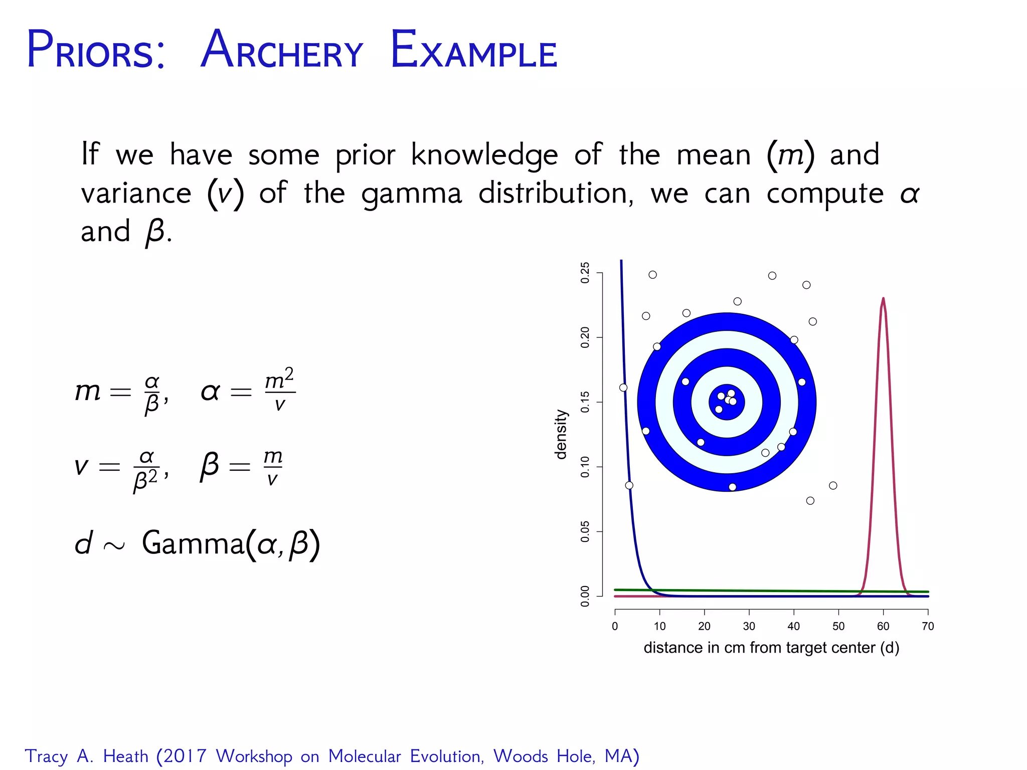
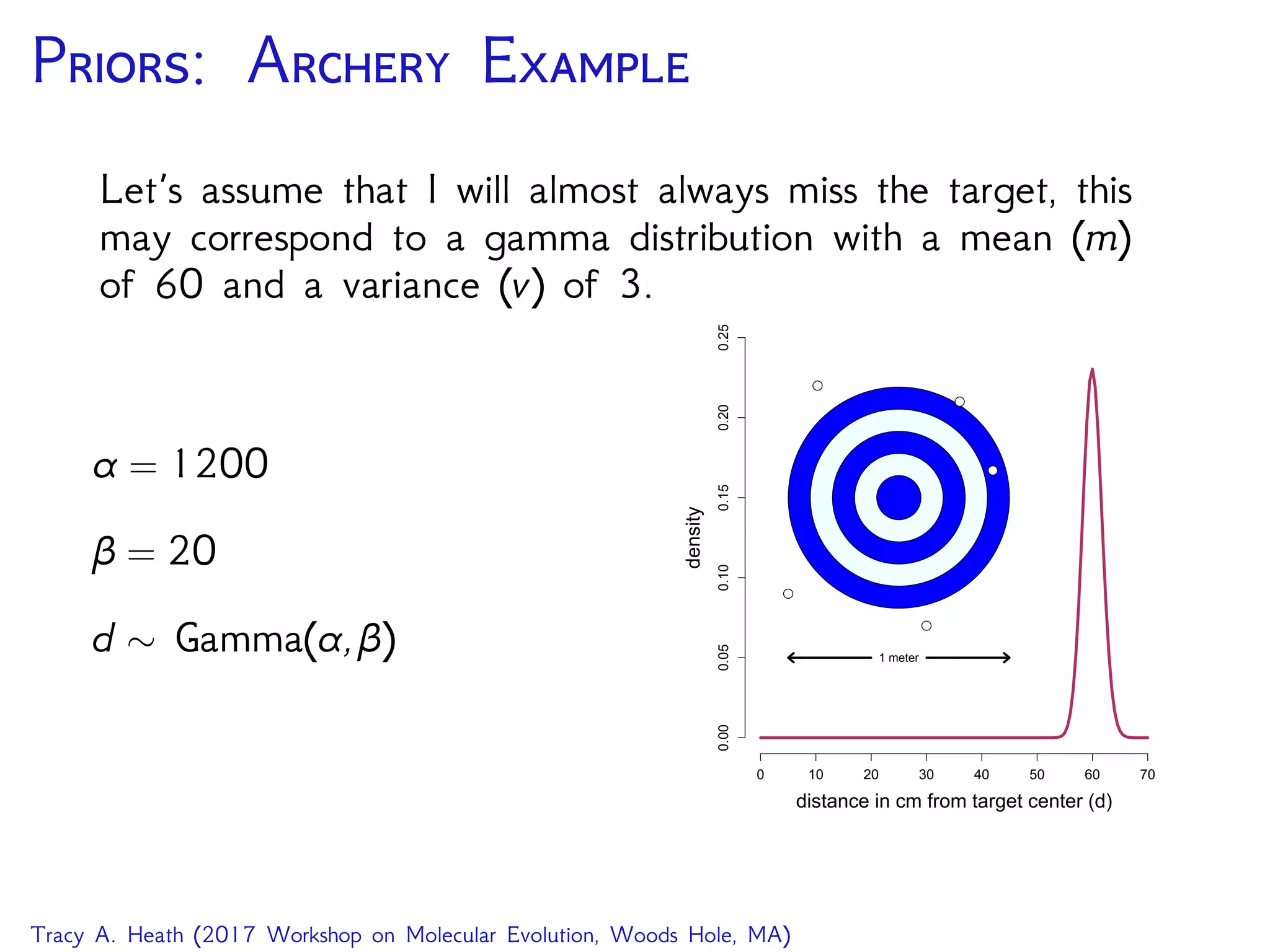
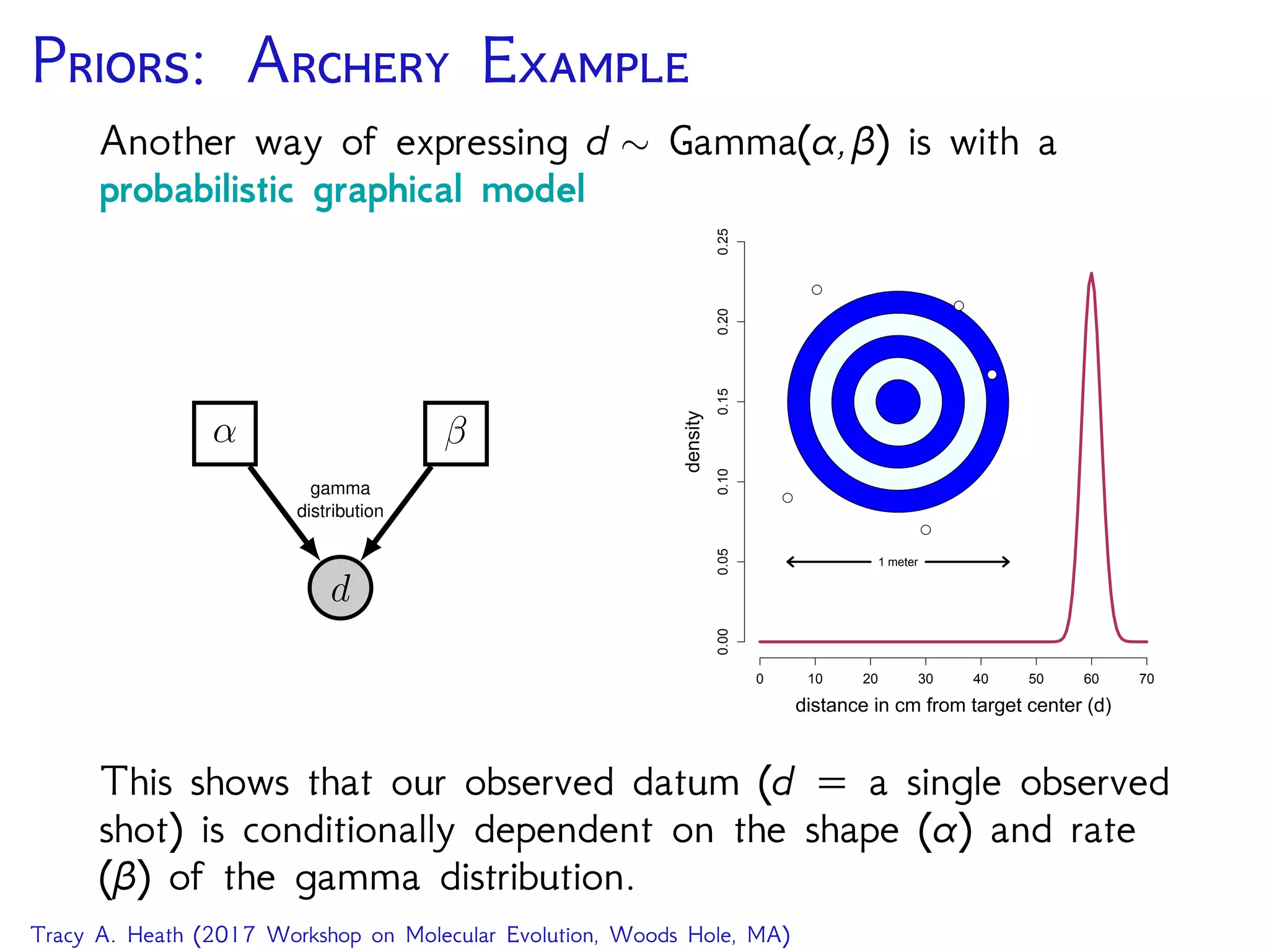
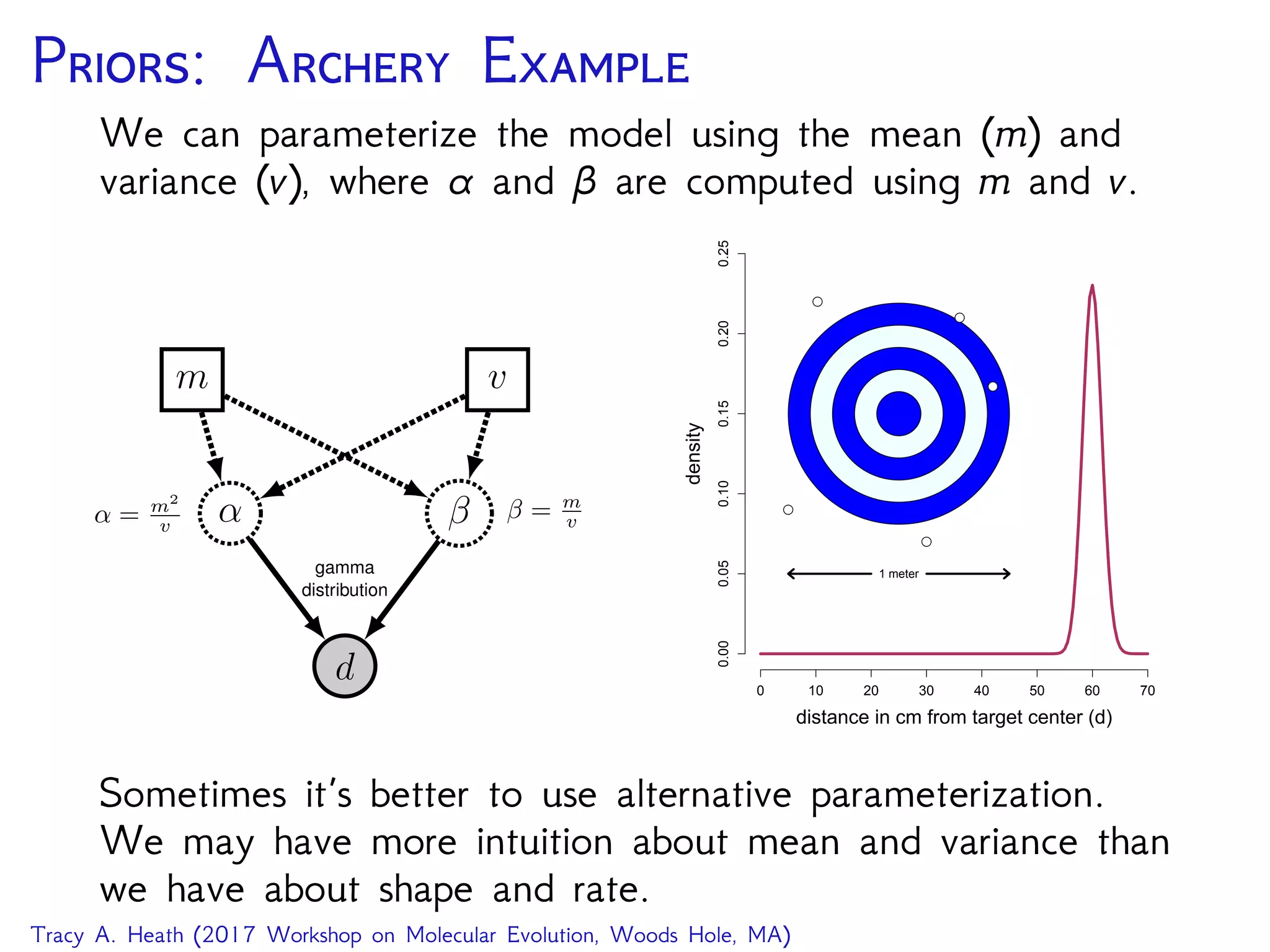
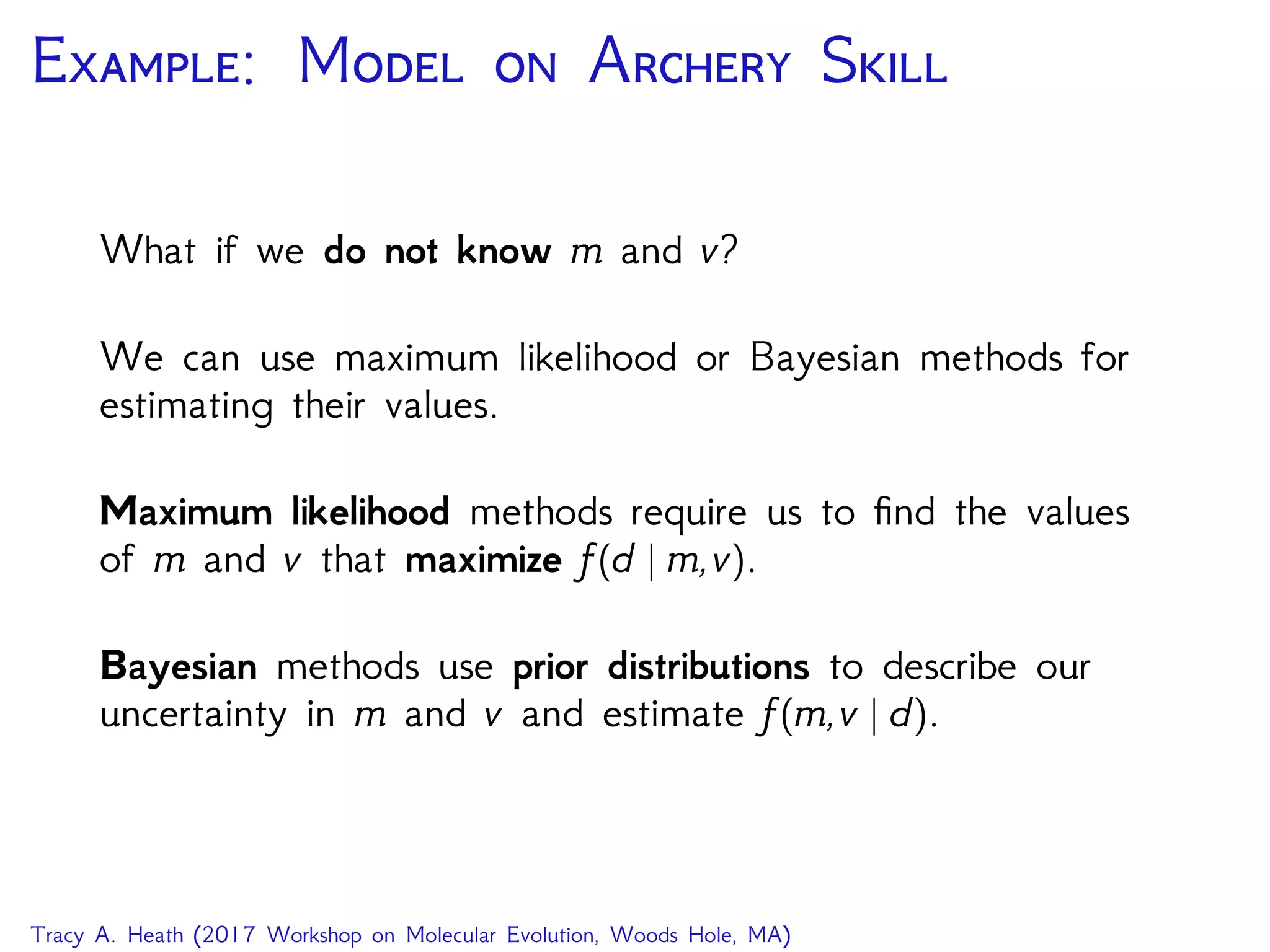
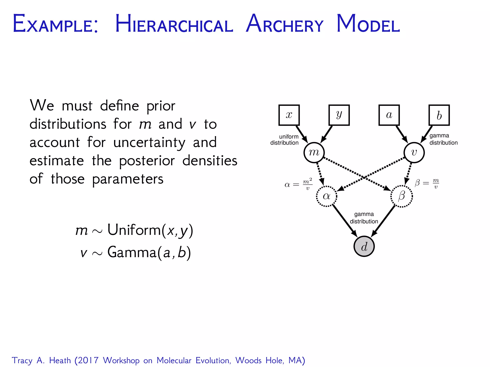
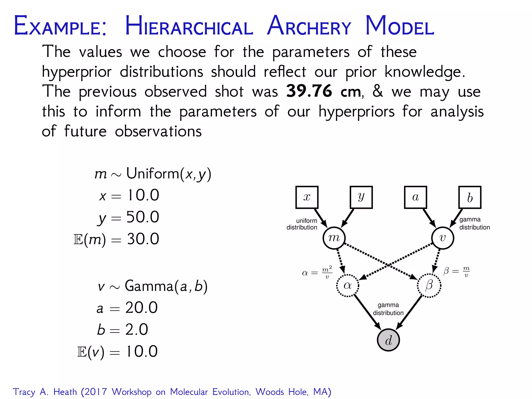
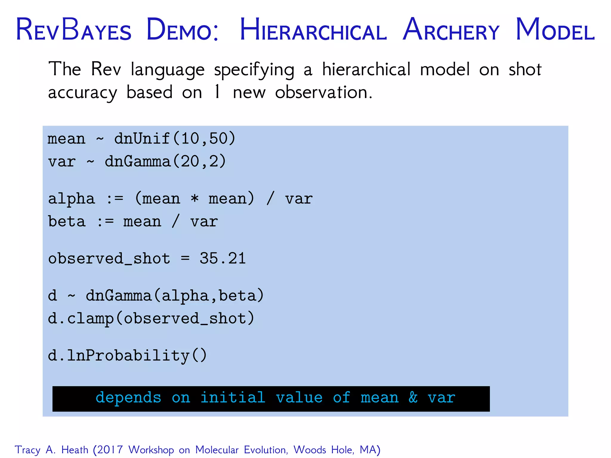
Download as PDF, PPTX

![RB D: H A M
The Rev language specifying the MCMC sampler for the
hierarchical model on archery accuracy.
... # model specification from previous demo
mymodel = model(beta)
moves[1] = mvSlide(mean,delta=1.0,tune=true,weight=3.0)
moves[2] = mvScale(var,lambda=1.0,tune=true,weight=3.0)
monitors[1] = mnModel(file="archery_mcmc_1.log",printgen=10, ...)
monitors[2] = mnScreen(printgen=1000, mean, var)
mymcmc = mcmc(mymodel, monitors, moves,nruns=1)
mymcmc.burnin(generations=10000,tuningInterval=1000)
mymcmc.run(generations=40000,underPrior=false)
MCMC screen output
Tracy A. Heath (2017 Workshop on Molecular Evolution, Woods Hole, MA)](https://image.slidesharecdn.com/heath-lecture1-170725113910/75/Integrative-Bayesian-Analysis-in-RevBayes-23-2048.jpg)
![B P
How is this applied to phylogenetic inference?
GTR on an unrooted tree
seq
PhyloCTMC
Q
GTRTree
bli ⌧
Exponential Uniform
10 N
i 2 2N 3
pi
Dirichlet
er
Dirichlet
↵2 ↵1
for (i in 1:n_branches) {
bl[i] ⇠ dnExponential(10.0)
}
topology ⇠ dnUniformTopology(taxa)
psi := treeAssembly(topology, bl)
alpha1 <- v(1,1,1,1,1,1)
alpha2 <- v(1,1,1,1)
er ⇠ dnDirichlet( alpha1 )
pi ⇠ dnDirichlet( alpha2 )
Q := fnGTR(er, pi)
seq ⇠ dnPhyloCTMC( tree=psi, Q=Q, pInv=p_invar,
siteRates=sr, type="DNA" )
seq.clamp( data )
(image source RevBayes Substitution Models Tutorial)
We can assemble a phylogenetic model in the same way,
using previously described models and probability
distributions as priors.
Tracy A. Heath (2017 Workshop on Molecular Evolution, Woods Hole, MA)](https://image.slidesharecdn.com/heath-lecture1-170725113910/75/Integrative-Bayesian-Analysis-in-RevBayes-30-2048.jpg)
![D: GTR T RB
GTR on an unrooted tree
seq
PhyloCTMC
Q
GTRTree
bli ⌧
Exponential Uniform
10 N
i 2 2N 3
pi
Dirichlet
er
Dirichlet
↵2 ↵1
for (i in 1:n_branches) {
bl[i] ⇠ dnExponential(10.0)
}
topology ⇠ dnUniformTopology(taxa)
psi := treeAssembly(topology, bl)
alpha1 <- v(1,1,1,1,1,1)
alpha2 <- v(1,1,1,1)
er ⇠ dnDirichlet( alpha1 )
pi ⇠ dnDirichlet( alpha2 )
Q := fnGTR(er, pi)
seq ⇠ dnPhyloCTMC( tree=psi, Q=Q, pInv=p_invar,
siteRates=sr, type="DNA" )
seq.clamp( data )
(image source RevBayes Substitution Models Tutorial)
Let’s step through this model and the MCMC in RevBayes!
Tracy A. Heath (2017 Workshop on Molecular Evolution, Woods Hole, MA)](https://image.slidesharecdn.com/heath-lecture1-170725113910/75/Integrative-Bayesian-Analysis-in-RevBayes-31-2048.jpg)

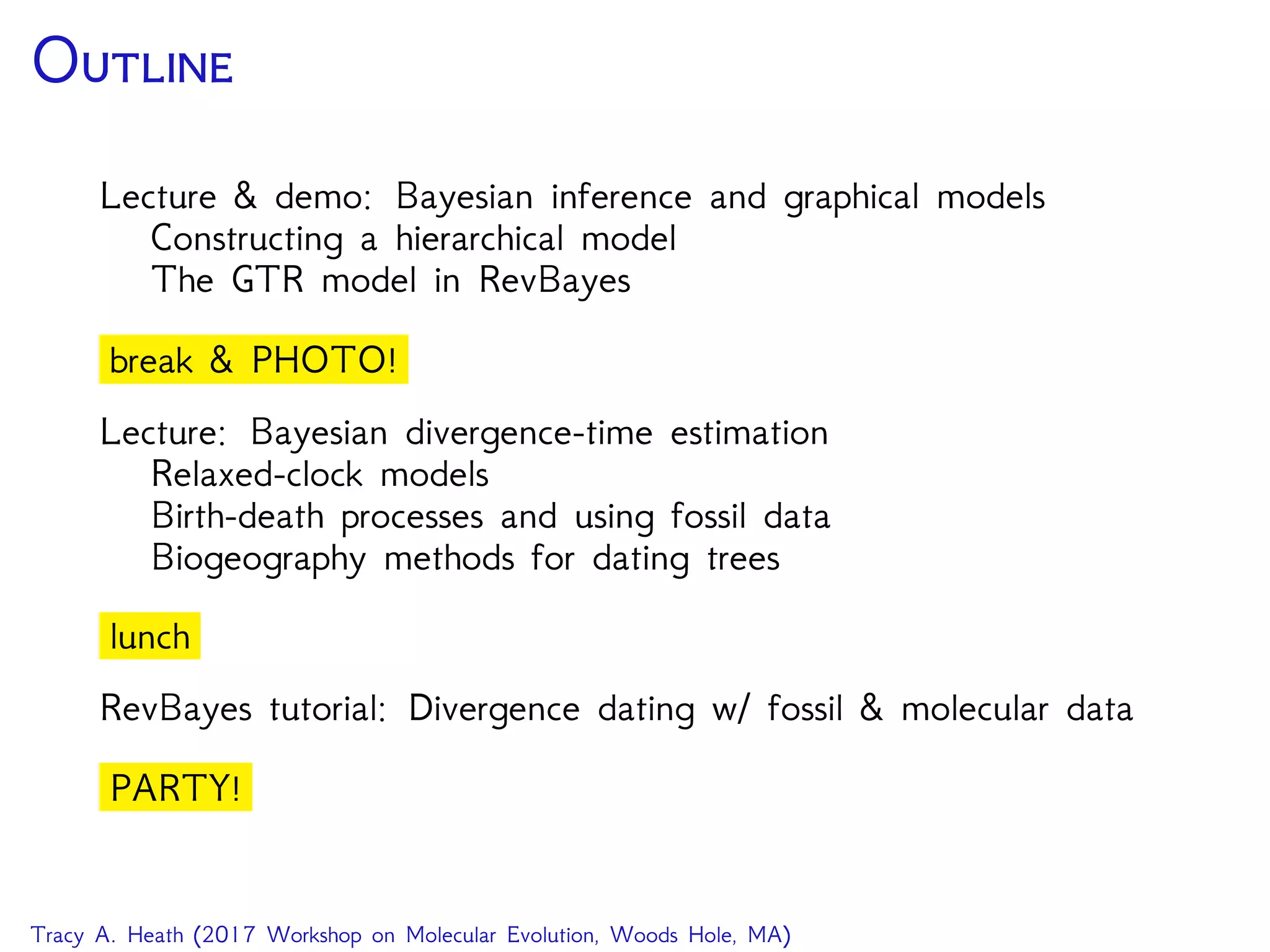
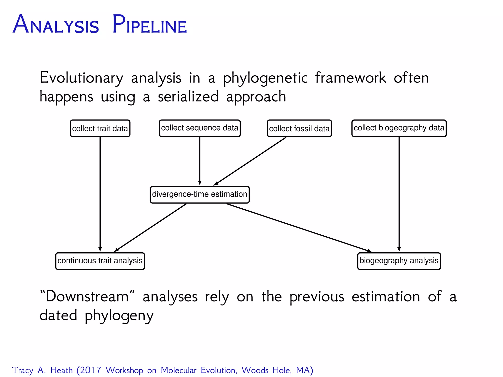
This document outlines a workshop presentation on integrative Bayesian analysis in RevBayes. The presentation includes an introduction to Bayesian inference using graphical models, constructing hierarchical models, and examples of divergence time estimation integrating molecular and fossil data. The agenda includes lectures on these topics as well as a hands-on tutorial using RevBayes to perform a divergence dating analysis with both molecular and fossil data and calibration points.