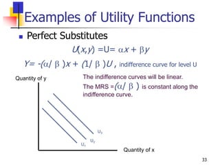
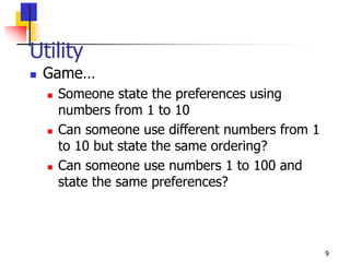
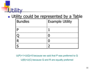
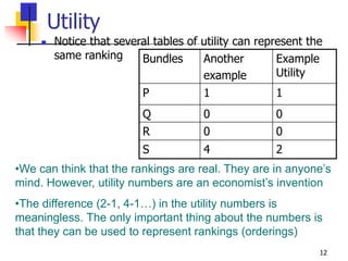
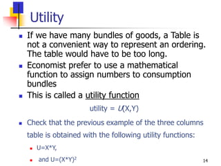
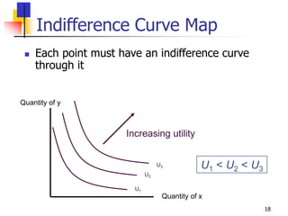
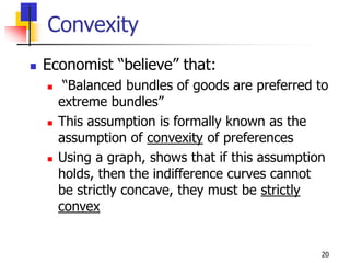
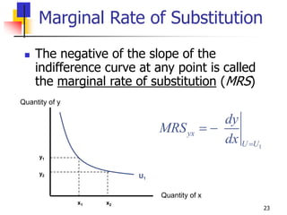
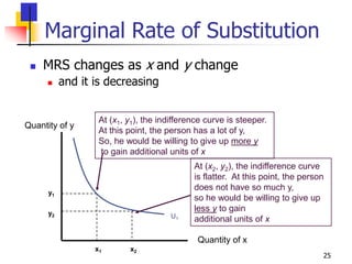
This document introduces the concept of utility and how it can be used to represent consumer preferences over bundles of goods. It discusses how utility rankings must satisfy certain axioms like completeness, transitivity, and continuity in order to be represented systematically. Utility is represented numerically using utility functions, with the rankings themselves being ordinal rather than cardinal. Indifference curves illustrate bundles that provide equal utility. The marginal rate of substitution measures how much of one good someone is willing to give up to obtain more of another good while maintaining the same utility. Utility functions take various forms, with Cobb-Douglas and perfect substitutes functions discussed as examples.

1. 1
Part 2
PREFERENCES AND UTILITY

2. 2
Objectives of the chapter
 Study a way to represent consumer’s
preferences about bundles of goods
 What are bundles of goods? =combinations of
goods. For instance:
 X=slices of pizza
 Y=glasses of juice
 Bundles:
 P: X=1, Y=1
 Q: X=3, Y=0
 R: Y=3, X=0
 S: X=2, Y=1

3. 3
Objectives of the chapter
 John’s preferences are such that:
 P is preferred to both Q and R
 S is preferred to P
 This way of representing preferences would be
very messy if we have many bundles
 In this chapter we study a simple way of
representing preferences over bundles of
goods
 This is useful because in reality there are
many bundles of goods

4. 4
Axioms of rational choice
 Before describing this simple method to
represent preferences over bundles, we will
study what requirements must the preferences
satisfy in order for the method to work
 These requirements are the axioms of rational
choice
 Without these requirements, it would be very
difficult to come up with a simple method to
represent preferences over many bundles of
goods
 It is easy to read a tube map, but not so much to
read a tube-bus-and rail map !!!!

5. 5
Axioms of Rational Choice
 Completeness
 if A and B are any two bundles, an
individual can always specify exactly one of
these possibilities:
 A is preferred to B
 B is preferred to A
 A and B are equally attractive
 In other words, preferences must exist in
order to be able to describe them through a
simple method

6. 6
Axioms of Rational Choice
 Transitivity
 if A is preferred to B, and B is preferred to
C, then A is preferred to C
 assumes that the individual’s choices are
internally consistent
 If transitivity does not hold, we would need
a very complicated method to describe
preferences over many bundles of goods

7. 7
Axioms of Rational Choice
 Continuity
 if A is preferred to B, then bundles suitably
“close to” A must also be preferred to B
 If this does not hold, we would need a very
complicated method to describe individual’s
preferences

8. 8
Utility
 Given these assumptions, it is possible to
show that people are able to rank all
possible bundles from least desirable to
most
 Economists call this ranking utility
 if A is preferred to B, then the utility assigned
to A exceeds the utility assigned to B
U(A) > U(B)

9. 9
Utility
 Game…
 Someone state the preferences using
numbers from 1 to 10
 Can someone use different numbers from 1
to 10 but state the same ordering?
 Can someone use numbers 1 to 100 and
state the same preferences?

10. 10
Utility
 Game…
 Clearly, the numbers are arbitrary
 The only consistent thing is the ranking that
we obtain

11. 11
Utility
 Utility could be represented by a Table
Bundles Example Utility
P 1
Q 0
R 0
S 2
U(P)=1>U(Q)=0 because we said that P was preferred to Q
U(B)=U(C) because Q and R are equally preferred

12. 12
Utility
 Notice that several tables of utility can represent the
same ranking Bundles Another
example
Example
Utility
P 1 1
Q 0 0
R 0 0
S 4 2
•We can think that the rankings are real. They are in anyone’s
mind. However, utility numbers are an economist’s invention
•The difference (2-1, 4-1…) in the utility numbers is
meaningless. The only important thing about the numbers is
that they can be used to represent rankings (orderings)

13. 13
Utility
 Utility rankings are ordinal in nature
 they record the relative desirability of commodity
bundles
 Because utility measures are not unique, it
makes no sense to consider how much more
utility is gained from A than from B. This gain in
utility will depend on the scale which is
arbitrary
 It is also impossible to compare utilities
between people. They might be using different
scales….

14. 14
Utility
 If we have many bundles of goods, a Table is
not a convenient way to represent an ordering.
The table would have to be too long.
 Economist prefer to use a mathematical
function to assign numbers to consumption
bundles
 This is called a utility function
utility = U(X,Y)
 Check that the previous example of the three columns
table is obtained with the following utility functions:
 U=X*Y,
 and U=(X*Y)2

15. 15
Utility
 Clearly, for an economist it is the same to use
U=X*Y than to use U=(X*Y)2 because both represent
the same ranking (see the table), so both functions will
give us the same answer in terms of which bundles of
good are preferred to others
 Any transformation that preserves the ordering
(multiply by a positive number, take it at a power of a
positive number, take “ln”) will give us the same
ordering and hence the same answer
 We can use this property to simplify some mathematical
computations that we will see in the future

16. 16
Economic Goods
 In the utility function, the x and y are
assumed to be “goods”
 more is preferred to less
Quantity of x
Quantity of y
x*
y*
Preferred to x*, y*
?
?
Worse
than
x*, y*

17. 17
Indifference Curves
 An indifference curve shows a set of
consumption bundles among which the
individual is indifferent
Quantity of x
Quantity of y
x1
y1
y2
x2
U1
Combinations (x1, y1) and (x2, y2)
provide the same level of utility

18. 18
Indifference Curve Map
 Each point must have an indifference curve
through it
Quantity of x
Quantity of y
U1 < U2 < U3
U1
U2
U3
Increasing utility

19. 19
Transitivity
 Can any two of an individual’s indifference
curves intersect?
Quantity of x
Quantity of y
U1
U2
A
B
C
The individual is indifferent between A and C.
The individual is indifferent between B and C.
Transitivity suggests that the individual
should be indifferent between A and B
But B is preferred to A
because B contains more
x and y than A

20. 20
Convexity
 Economist “believe” that:
 “Balanced bundles of goods are preferred to
extreme bundles”
 This assumption is formally known as the
assumption of convexity of preferences
 Using a graph, shows that if this assumption
holds, then the indifference curves cannot
be strictly concave, they must be strictly
convex

21. 21
Convexity
 Formally, If the indifference curve is convex, then the combination
(x1 + x2)/2, (y1 + y2)/2 will be preferred to either (x1,y1) or (x2,y2)
Quantity of x
Quantity of y
U1
x2
y1
y2
x1
This means that “well-balanced” bundles are preferred
to bundles that are heavily weighted toward one
Commodity (“extreme bundles”).
The middle points are better than the
Extremes, so the middle is at a higher indifference
Curve.
(x1 + x2)/2
(y1 + y2)/2

22. 22
Marginal Rate of Substitution
 Important concept !!
 MRSYX is the number of units of good Y
that a consumer is willing to give up in
return for getting one more unit of X in
order to keep her utility unchanged
 Let’s do a graph in the whiteboard !!!
 MRSYX is the negative of the slope of the
indiference curve (where Y is in the
ordinates axis)

23. 23
Marginal Rate of Substitution
 The negative of the slope of the
indifference curve at any point is called
the marginal rate of substitution (MRS)
Quantity of x
Quantity of y
x1
y1
y2
x2
U1
1
yx
U U
dy
MRS
dx 
 

24. 24
Marginal Rate of Substitution
 Notice that if indifference curves are strictly
convex, then the MRS is decreasing (as x
increases, the MRSyx decreases)
 See it in a graph: As “x” increases, the amount
of “y” that the consumer is gives up to stay in
the same indifference curve (that is MRSyx)
decreases
 If the assumption that “balanced bundles” are
preferred to “extreme bundles” (convexity of
preferences assumption” holds then the MRSyx
is decreasing!!

25. 25
Marginal Rate of Substitution
 MRS changes as x and y change
 and it is decreasing
Quantity of x
Quantity of y
x1
y1
y2
x2
U1
At (x1, y1), the indifference curve is steeper.
At this point, the person has a lot of y,
So, he would be willing to give up more y
to gain additional units of x
At (x2, y2), the indifference curve
is flatter. At this point, the person
does not have so much y,
so he would be willing to give up
less y to gain
additional units of x

26. 26
Utility and the MRS
 Suppose an individual’s preferences for
hamburgers (y) and soft drinks (x) can
be represented by
y
x 

10
utility
Solving for y, we get the indifference curve for level 10:
y = 100/x
• Taking derivatives, we get the MRS = -
dy/dx:
MRS = -dy/dx = 100/x2

27. 27
Utility and the MRS
MRSyx = -dy/dx = 100/x2
 Note that as x rises, MRS falls
 when x = 5, MRSyx = 4
 when x = 20, MRSyx = 0.25
 When x=20, then the individual does not
value much an additional unit of x. He is only
willing to give 0.25 units of y to get an
additional unit of x.

28. 28
Another way of computing the MRS
 Suppose that an individual has a utility
function of the form
utility = U(x,y)
 The total differential of U is
dy
y
U
dx
x
U
dU






Along any indifference curve, utility is constant (dU = 0)
dU/dy and dU/dx are the marginal utility of y and x
respectively

29. 29
Another way of computing the MRS
 Therefore, we get:
U constant
yx
U
dy x
MRS
U
dx
y



  


MRS is the ratio of the marginal utility of x to the marginal
utility of y
Marginal utilities are generally positive (goods)

30. 30
Example of MRS
 Suppose that the utility function is
y
x 

utility
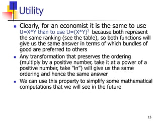
We can simplify the algebra by taking the logarithm of this
function (we have explained before that taking the logarithm
does not change the result because it preserves the ordering,
though it can make algebra easier)
U*(x,y) = ln[U(x,y)] = 0.5 ln x + 0.5 ln y

31. 31
Deriving the MRS
* 0.5
* 0.5
yx
U
y
x x
MRS
U x
y y


  


 Thus,
Notice that the MRS is decreasing in x: The MRS
falls when x increases

32. 32
Examples of Utility Functions
 Cobb-Douglas Utility
utility = U(x,y) = xy
where  and  are positive constants
 The relative sizes of  and  indicate the relative
importance of the goods
 The algebra can usually be simplified by taking
ln(). Let’s do it in the blackboard….

33. 33
Examples of Utility Functions
 Perfect Substitutes
U(x,y) =U= x + y
Y= -(/  )x + (1/  )U , indifference curve for level U
Quantity of x
Quantity of y
U1
U2
U3
The indifference curves will be linear.
The MRS =(/  ) is constant along the
indifference curve.

34. 34
Examples of Utility Functions
 Perfect Substitutes
U(x,y) =U= x + y
dU= dx + dy
 Notice that the change in utility will be the
same if (dx=  and dy= 0) or if (dx= 0 and
dy= ). So x and y are exchanged at a fixed
rate independently of how much x and y the
consumer is consumed
 It is as if x and y were substitutes. That is
why we call them like that

35. 35
Examples of Utility Functions
 Perfect Complements
utility = U(x,y) = min (x, y)
Quantity of x
Quantity of y
The indifference curves will be
L-shaped. It is called complements
because if we
Are in the kink then utility does not
increase by we increase the quantity
of only one good. The quantity of both
Goods must increase in order to increase
utility
U1
U2
U3

36. 36
Examples of Utility Functions
 CES Utility (Constant elasticity of
substitution)
utility = U(x,y) = x/ + y/
when   0 and
utility = U(x,y) = ln x + ln y
when  = 0
 Perfect substitutes   = 1
 Cobb-Douglas   = 0
 Perfect complements   = -

37. 37
Examples of Utility Functions
 CES Utility (Constant elasticity of
substitution)
 The elasticity of substitution () is equal to
1/(1 - )
 Perfect substitutes   = 
 Fixed proportions   = 0