This paper presents a modification of the deep Q-network (DQN) in deep reinforcement learning to control the angle of the inverted pendulum (IP). The original DQN method often uses two actions related to two force states like constant negative and positive force values which apply to the cart of IP to maintain the angle between the pendulum and the Y-axis. Due to the changing of too much value of force, the IP may make some oscillation which makes the performance system could be declined. Thus, a modified DQN algorithm is developed based on neural network structure to make a range of force selections for IP to improve the performance of IP. To prove our algorithm, the OpenAI/Gym and Keras libraries are used to develop DQN. All results showed that our proposed controller has higher performance than the original DQN and could be applied to a nonlinear system.

1. International Journal of Electrical and Computer Engineering (IJECE)
Vol. 13, No. 4, August 2023, pp. 3895~3902
ISSN: 2088-8708, DOI: 10.11591/ijece.v13i4.pp3895-3902  3895
Journal homepage: http://ijece.iaescore.com
Development of deep reinforcement learning for inverted
pendulum
Khoa Nguyen Dang1
, Van Tran Thi2
, Long Vu Van3
1
Faculty of Applied Sciences, International School, Vietnam National University, Hanoi, Vietnam
2
Faculty of General Education, University of Labour and Social Affairs, Hanoi, Vietnam
3
Shinka Network PTE, Hanoi, Vietnam
Article Info ABSTRACT
Article history:
Received Dec 27, 2021
Revised Nov 21, 2022
Accepted Dec 7, 2022
This paper presents a modification of the deep Q-network (DQN) in deep
reinforcement learning to control the angle of the inverted pendulum (IP).
The original DQN method often uses two actions related to two force states
like constant negative and positive force values which apply to the cart of IP
to maintain the angle between the pendulum and the Y-axis. Due to the
changing of too much value of force, the IP may make some oscillation
which makes the performance system could be declined. Thus, a modified
DQN algorithm is developed based on neural network structure to make a
range of force selections for IP to improve the performance of IP. To prove
our algorithm, the OpenAI/Gym and Keras libraries are used to develop
DQN. All results showed that our proposed controller has higher performance
than the original DQN and could be applied to a nonlinear system.
Keywords:
Deep Q-network
Inverted pendulum
Neural network
OpenAI/Gym
Reinforcement learning This is an open access article under the CC BY-SA license.
Corresponding Author:
Khoa Nguyen Dang
Faculty of Applied Sciences, International School, Vietnam National University
144 Xuan Thuy Road, Cau Giay, Hanoi 100000, Vietnam
Email: khoand@vnuis.edu.vn
1. INTRODUCTION
An inverted pendulum (IP) system consists of a pendulum mounted on a cart pole. The goal is to
maintain an angle between the pendulum and Y-axis by applying a force to the cart. This system is often
considered a highly unstable system and difficult to control which becomes a classical problem in the control
system domain.
In the last few years, many researchers have applied many well-known controllers such as
proportional integral derivative (PID), linear quadratic regulator (LQR), sliding mode control (SMC), and
fuzzy to achieve the stabilization control of the IP system. Herein, PID [1], [2] and LQR [3]–[5] are two
popular controller methods that show great stabilization in many linear systems. The PID and LQR controller
still have some disadvantages in controlling nonlinear systems like IP that need to be improved such as the
settling time and overshoot percentage. Besides, SMC is a very powerful method in eliminating nonlinear
systems. Many researchers [6]–[9] had presented the SMC for an IP system. Although the overshoot is
decreased significantly, the control design is still complex and special to the chattering phenomenon problem.
While fuzzy logic [10], LQR-PID [11], [12], and fuzzy-PID [13] have been considered to improve the
performance of IP controllers. However, the equation computations are extremely complicated.
Besides the above traditional controller, some advanced controls are developed like adaptive control
[14], [15] and robust control [16]. These results satisfied the basic requirement for the IP system, which gets
higher performance than the traditional technique. But their design control and equation have still complex to
apply to many different systems.

2.  ISSN: 2088-8708
Int J Elec & Comp Eng, Vol. 13, No. 4, August 2023: 3895-3902
3896
Nowadays, deep learning (DL) is the new method to make the controller more and more intelligent.
The neural network (NN) could help the system to improve its self-learning in getting to the desired goal. For
IP systems, many articles found out that robustness and effectiveness when using NN such as radial basis
function (RBF) or multilayer feedforward neural network (MLFF NN) to control IP systems [17], [18]. Some
researchers [19], [20] had also applied the fuzzy with neural networks but the networks are simple.
For the complexity of a non-linear and unstable, deep reinforcement learning (DRL) becomes
well-known in building an intelligent system to solve very complicated problems based on its experiment
in a specific environment, which had shown robustness [21]–[23] with different algorithms such as deep
Q-networks (DQN), deep deterministic policy gradient (DDPG), proximal policy optimization (PPO).
Each algorithm has advantages and disadvantages for various situations. Besides, DRL is combined with
the original control algorithm like PID-based DRL [24], reference signal self-organizing control system
based DRL [25]. All presentations have given well results which could maintain the pendulum angle close
to zero degrees. However, DQN for the inverse pendulum generates the force control for the cart with two
values (two outputs from NN) the positive force and negative force [26], [27] related to two actions of
DRL which is decided by a neural network. The changing force with a high range may make the
oscillation of the cart effect. Therefore, this paper will develop a DQN algorithm for controlling the angle
of the inverted pendulum system using a small range of force by many outputs from NN values to reduce
oscillation based on the NN structure. Fully, the performance of IP is improved significantly. The
algorithm results are presented based on the OpenAI/Gym and Keras libraries.
The paper is organized as: firstly, we are going to present the model configuration and the
mathematic equation of the IP system in section 2. Secondly, we introduce the reinforcement learning
method and DQN in section 3. Then, the performance of our proposal is presented and compared to the
original methods in section 4. Finally, the conclusions are given in section 5.
2. METHOD
2.1. Inverse pendulum modeling
The model of an inverted pendulum is described in Figure 1. In general, the IP consists of a
pendulum on the top of the cart while moving forward/backward along the rail and the pendulum can move
freely around the joint between it and the cart. The dynamical equation of the IP system [28] can be presented
as (1) and (2), where the parameters are defined in Table 1. To maintain the desired angle between the
pendulum and Y-axis, the DRL is developed to generate 𝐹𝑎 for the cart based on deep reinforcement learning,
which is presented in the next section.
𝜃̈ =
𝑔𝑐 (𝑀+𝑚)𝑠𝑖𝑛 𝜃 −(𝐹𝑎+𝑚 𝑙 𝜃2
̇ 𝑠𝑖𝑛 𝜃 )𝑐𝑜𝑠 𝜃
𝑙 (
4
3
(𝑀+𝑚)−𝑚𝜃 )
(1)
𝑥̈ =
𝐹𝑎+𝑚 𝑙 (𝜃2
̇ 𝑠𝑖𝑛 𝜃 −𝜃̈ 𝑐𝑜𝑠 𝜃 )
𝑀+𝑚
(2)
Figure 1. IP modeling
Table 1. The parameters of inverse pendulum
Parameters Meaning Unit
M Mass of cart kg
m Mass of pendulum kg
𝜃 Angle of pendulum degree
x Position of Cart m
l Half of the length pendulum m
Fa Force to cart N
gc Acceleration of gravity m/s2

3. Int J Elec & Comp Eng ISSN: 2088-8708 
Development of deep reinforcement learning for inverted pendulum (Khoa Nguyen Dang)
3897
2.2. Reinforcement learning
Reinforcement learning (RL) is a type of machine learning in which its concept is trial and error.
Objects using RL can learn from their experience in an environment. A typical model using RL is described
in Figure 2.
Figure 2. Reinforcement learning diagram
RL contains two main components: agent and environment. Herein, the environment uses the input
action 𝑎(𝑡) from agent to generate a state 𝑠(𝑡) and reward 𝑟(𝑡) which are sent back to the agent. An algorithm
is developed in the agent to find the best action based on the policy 𝜋 which goal aims to achieve maximum
reward in return. RL becomes a closed loop between the environment and the agent. Each loop is called a
step. Let us define an episode containing N steps. The training process will be performed within 𝑁𝑥𝑀 loop
times where N is the number step and M is the number of episodes as below code example.
For i in range(M): //Loop episode
Reset state (s(t)) of environment to initial
For j in range(N): // Loop N steps
// Send state (s(t)) to Agent
// Using policy to generate action a(t)
// Send action to Environment
// Environment will create new states s(t+1)
// Environment uses some conditions to create the reward r(t)
// if ((theta>-12) and (theta<12)) reward+=1 else reward +=0; break;
//Update policy based on state and action
Normally, RL uses the Epsilon-greedy method [29], [30] as the policy to generate the action. This
policy can use a table named Q-table as the reference which shows the relationship between the state and the
action. Each value in Q-table is called by Q-value 𝑄(𝑠𝑗, 𝑎𝑖) where j=(1, 2, … m) and i=(1, 2, … n). For
example, Q-table is shown in Table 2. And the selected action can be given by the policy as in (3). Where 𝜀
is the probability in selection random action, with a range from 0 to 1. The main purpose of RL is to find the
maximum total reward based on policy. The updated policy is very important to select the best action for the
environment, which can be applied [31] as Bellman equation in (4).
𝑎(𝑡) = {
𝑎𝑖 at max 𝑄(𝑠𝑖, 𝑎𝑗) 𝑤𝑖𝑡ℎ 𝑝𝑟𝑜𝑏𝑎𝑏𝑖𝑙𝑖𝑡𝑦 (1 − 𝜀)
𝑎𝑟 at 𝑅𝑎𝑛𝑑𝑜𝑚 𝑎𝑐𝑡𝑖𝑜𝑛 𝑤𝑖𝑡ℎ 𝑝𝑟𝑜𝑏𝑎𝑏𝑖𝑙𝑖𝑡𝑦 𝜀
(3)
𝑄𝑛𝑒𝑤(𝑠(𝑡), 𝑎(𝑡)) ← 𝑟(𝑡+1) + 𝛾 max(𝑄(𝑠(𝑡+1), 𝑎(𝑡+1))) (4)
where 𝑄𝑛𝑒𝑤(𝑠(𝑡), 𝑎(𝑡)) is the new Q-value at time t, 𝛾 is discount factor, range value from 0 to 1, 𝑟(𝑡+1) is
reward obtained with state 𝑠(𝑡+1) at time (t+1), 𝑎(𝑡+1) is the action in time (t+1), max (𝑄(𝑠(𝑡+1), 𝑎(𝑡+1))) is
the maximum of Q-value target gets in the next state 𝑠(𝑡+1) with action 𝑎(𝑡+1) at the time (t+1).
Table 2. Q-table of RL
Action 1 Action 2 .... Action n
State 1 𝑄(𝑠1, 𝑎1) 𝑄(𝑠1, 𝑎2) ... 𝑄(𝑠1, 𝑎𝑛)
State 2 𝑄(𝑠2, 𝑎1) 𝑄(𝑠2, 𝑎2) … 𝑄(𝑠2, 𝑎𝑛)
State ... … … … …
State m 𝑄(𝑠𝑚, 𝑎1) 𝑄(𝑠𝑚, 𝑎2) … 𝑄(𝑠𝑚, 𝑎𝑛)
Based on the current state 𝑠(𝑡), the agent has to generate the new action 𝑎(𝑡) using the policy in (3)
which will send to Environment to make the new state 𝑠(𝑡+1) and new reward 𝑟(𝑡+1). This state 𝑠𝑡+1 is used to

4.  ISSN: 2088-8708
Int J Elec & Comp Eng, Vol. 13, No. 4, August 2023: 3895-3902
3898
find 𝑚𝑎𝑥 (𝑄(𝑠(𝑡+1), 𝑎(𝑡+1))) in (4) among all Q-values 𝑄(𝑠(𝑡+1), 𝑎𝑖) which relates to actions 𝑎𝑖 in Table 2
with i=(1, 2,…, n). Therefore, the 𝑄𝑛𝑒𝑤(𝑠(𝑡), 𝑎(𝑡)) in (4) is computed and updated into Q-table on position
Q(𝑠(𝑡), 𝑎(𝑡)).
Many applications require a lot of actions and states. The size of the Q-table will be extremely large
and consume lots of time and resources in calculating Q-value. Therefore, DQN is one solution to overcome
the limitations of the Q-table, which is presented in the next content.
2.3. Deep Q-network
Deep Q-networks (DQN) uses NN to approximate Q-value 𝑄(𝑠(t), 𝑎(t)) instead of using the Q-table
in the RL method. This NN will make one model named the prediction model (PM) which contains three
layers that are the input layer (the current state of the environment), the hidden layer (computations with
activation function), and the output layer (predict the Q-value). The DQN model is shown in Figure 3.
Figure 3. DQN model using a neural network
Instead of finding 𝑚𝑎𝑥 (𝑄(𝑠(𝑡+1), 𝑎(𝑡+1))) in 4 from Table 1, another NN named the target model
(TM) is used to estimate this value and then substitute it into 4 to computed 𝑄𝑛𝑒𝑤_𝑒𝑞(𝑠(𝑡), 𝑎(𝑡)):
𝑄𝑛𝑒𝑤_𝑒𝑞(𝑠(𝑡), 𝑎(𝑡)) =𝑟(𝑡+1) + 𝛾 𝑚𝑎𝑥 (𝑄(𝑠(𝑡+1), 𝑎(𝑡+1))). On the other hand, TM has also defined the same
architecture network with PM which is developed to estimate the 𝑄𝑛𝑒𝑤_𝑒𝑞(𝑠(𝑡), 𝑎(𝑡)) [21]. The error between
𝑄𝑛𝑒𝑤_𝑒𝑞(𝑠(𝑡), 𝑎(𝑡)) and 𝑄𝑛𝑒𝑤_𝑁𝑁(𝑠(𝑡), 𝑎(𝑡)) will be used to update the PM’s weight using the gradient descent
method. The loss function for updating can be defined as (5).
𝐿𝑜𝑠𝑠 = [ 𝑄𝑛𝑒𝑤_𝑒𝑞(𝑠(𝑡), 𝑎(𝑡)) − 𝑄𝑛𝑒𝑤_𝑁𝑁(𝑠(𝑡), 𝑎(𝑡))]
2
(5)
To apply the training process, a set of training data need to be created. In the initial, a random state
and reward are generated and sent to the agent (including PM and policy) as in Figure 4. Herein, the PM is
used to predict the Q-values 𝑄𝑛𝑒𝑤_𝑁𝑁(𝑠(𝑡)𝑗, 𝑎(𝑡)𝑖) and use the policy in (3) to select the best action for the
environment. Therefore, the environment will have a new state and reward to make a closed loop. Let us
define N loop times, a set of training data in the form 𝐸(𝑡) = (𝑠(𝑡) , 𝑎(𝑡) , 𝑟(𝑡+1) , 𝑠(𝑡+1)) is stored into
experience replay (ER), which is applied in the training step as Figure 5. Next, let us define the inputs of TM
and PM. One random sample 𝐸(𝑡) in ER is selected for TM and PM with 𝑠(𝑡) and 𝑠(𝑡+1), respectively.
Therefore, we can be given the output the 𝑄𝑛𝑒𝑤_𝑒𝑞(𝑠(𝑡), 𝑎(𝑡)) and 𝑄𝑛𝑒𝑤_𝑁𝑁(𝑠(𝑡), 𝑎(𝑡)) for (5).
In this paper, we propose a modification of the DQN method by increasing the output of the neural
network model. It makes the IP system more and more stable and easy to reach an upright position (𝜃 = 0).
To demonstrate this, we create the IP environment based on OpenAI/Gym which is open-source and apply
the DQN algorithm with different number outputs for the agent part in RL to control IP maintenance with an
angle. The simulation and result will be performed and discussed in the next section.

5. Int J Elec & Comp Eng ISSN: 2088-8708 
Development of deep reinforcement learning for inverted pendulum (Khoa Nguyen Dang)
3899
Figure 4. RL using the DQN method Figure 5. Training DQN process
3. RESULTS AND DISCUSSION
In this section, our proposal is performed to demonstrate the performance of IP. Firstly, let us define
the parameters of IP as in Table 3. Secondly, from (1), the output states of environment are defined as four
parameters: [𝑥, 𝑥̇, 𝜃, 𝜃̇]. Where 𝑥̇ is the linear velocity of the cart (m/s) along the rail and the 𝜃̇ is the angular
velocity (rad/s). Next, we define the condition to decide the reward as in (6). Thirdly, the agent will generate
the action, which is presented by the neural network. Three cases with different numbers of output nodes are
shown in Table 4, which contain 2, 3, and 17 outputs from the neural network.
𝑟𝑒𝑤𝑎𝑟𝑑 = {
1 𝑖𝑓 − 12 < 𝜃 < 12
0 𝑖𝑓 𝜃 < −12 𝑜𝑟 𝜃 > 12
(6)
Table 3. The special parameters of the inverse pendulum
Parameters Values
M 1.0
m 0.1
l 0.5
Fa 8.0
gc 9.8
Table 4. Neural network configuration in three cases
Name Model 1 Model 2 Model 3 (our proposal)
Number of inputs 4 4 4
Number of hidden layers 4 4 4
Number of the node in each hidden layer 18 18 18
Number of outputs 2 3 17
Training steps 70,000 70,000 70,000
Fourthly, each model will be trained in 70,000 steps. In the training step, the cart-pole system will
be terminated if its angle is greater than 12 degrees or less than -12 degrees. Figure 6 shows the total reward
value obtained from each episode while training three models in 70,000 steps. Herein, Figures 6(a) to 6(c)
present for each case of model 1, model 2, and model 3, respectively which are described in Table 4. For
clearly, we computed the average reward in the last 50 episodes (blue line). Because the DQN model learns
based on the trial-and-error process, so the total reward could change based on ratio error and success in the
trial process. All steps are performed on a computer with the specification as CPU (Intel Core i7-7500U
2.7 GHz (4CPUs)), GPU (NVIDIA GEFORCE MX150, 2 GB), RAM (12 GB), HDD (256 GB).
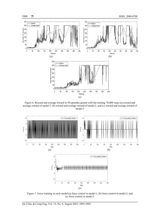
Next, the testing step will use the NN which is trained in the previous step. Herein, the weight of
NN is often updated for each training step. All models are tested during 400 steps with the initial angle of the
pendulum at 17 degrees and the desired angle is 0 degrees.
As the results in Figures 7(a) and 7(b), the forces in model 1 and model 2 are only selected by
(–𝐹𝑎, 𝐹𝑎) and (–𝐹𝑎, 0, 𝐹𝑎), respectively. Because the force applied to the cart-pole in each step is very high
(either –𝐹𝑎/𝐹𝑎 and –𝐹𝑎/0/𝐹𝑎) which affects the cart pole by some oscillation as in Figure 7(c). It means that the
performance of IP is weakened. Model 3 makes the force-like continuously (-𝐹𝑎, -𝐹𝑎+1, -𝐹𝑎+2, ..., 0, 1, 2, ...,
𝐹𝑎) corresponded to 17 outputs of NN, which could reduce oscillation for the cart pole and the system has
higher performance than model 1 and model 2. Furthermore, model 3 has a lower overshot and quickly
makes a stable system than other models as in Figure 8. The cart pole could maintain desired angle
(0 degrees) of the pendulum.

6.  ISSN: 2088-8708
Int J Elec & Comp Eng, Vol. 13, No. 4, August 2023: 3895-3902
3900
(a) (b)
(c)
Figure 6. Reward and average reward in 50 episodes gained with the training 70,000 steps (a) reward and
average reward of model 1, (b) reward and average reward of model 2, and (c) reward and average reward of
model 3
(a) (b)
(c)
Figure 7. Force tracking in each model (a) force control in model 1, (b) force control in model 2, and
(c) force control in model 3

7. Int J Elec & Comp Eng ISSN: 2088-8708 
Development of deep reinforcement learning for inverted pendulum (Khoa Nguyen Dang)
3901
Figure 8. Response angle in each model
4. CONCLUSION
This paper presents the method for controlling the inverted pendulum based on DQN in DRL. By
creating a different number of outputs of NN in DQN, our proposal used 17 outputs that have higher
performance than the original DQN method using two and three outputs. All results showed that the angle of
IP reaches the desired value with zeros degree very fast and more stable. This proposed controller could
provide well performance for nonlinear systems of IP and other systems. In the future, a real system of the
inverse pendulum will be developed and applied DQN for controlling the angle of the pendulum as well as
the position of the cart.
REFERENCES
[1] K. Razzaghi and A. A. Jalali, “A new approach on stabilization control of an inverted pendulum, using PID controller,” Advanced
Materials Research, vol. 403–408, pp. 4674–4680, Nov. 2011, doi: 10.4028/www.scientific.net/AMR.403-408.4674.
[2] R. Mondal, J. Dey, S. Halder, and A. Chakraborty, “Stabilization of the cart-inverted pendulum system using PI λ D μ controller,”
in 2017 4th IEEE Uttar Pradesh Section International Conference on Electrical, Computer and Electronics (UPCON), Oct. 2017,
pp. 273–279, doi: 10.1109/UPCON.2017.8251060.
[3] E. V. Kumar and J. Jerome, “Robust LQR controller design for stabilizing and trajectory tracking of inverted pendulum,”
Procedia Engineering, vol. 64, pp. 169–178, 2013, doi: 10.1016/j.proeng.2013.09.088.
[4] H. Wang, H. Dong, L. He, Y. Shi, and Y. Zhang, “Design and simulation of LQR controller with the linear inverted pendulum,”
in 2010 International Conference on Electrical and Control Engineering, Jun. 2010, pp. 699–702, doi: 10.1109/iCECE.2010.178.
[5] H. X. Cheng, J. X. Chen, J. Li, and L. Cheng, “Optimal control for single inverted pendulum based on linear quadratic regulator,”
MATEC Web of Conferences, vol. 44, Mar. 2016, doi: 10.1051/matecconf/20164402064.
[6] R. Coban and B. Ata, “Decoupled sliding mode control of an inverted pendulum on a cart: An experimental study,” in 2017 IEEE
International Conference on Advanced Intelligent Mechatronics (AIM), Jul. 2017, pp. 993–997, doi: 10.1109/AIM.2017.8014148.
[7] J. Huang, Z.-H. Guan, T. Matsuno, T. Fukuda, and K. Sekiyama, “Sliding-mode velocity control of mobile-wheeled inverted-
pendulum systems,” IEEE Transactions on Robotics, vol. 26, no. 4, pp. 750–758, Aug. 2010, doi: 10.1109/TRO.2010.2053732.
[8] Z. Liu, F. Yu, and Z. Wang, “Application of sliding mode control to design of the inverted pendulum control system,” in
2009 9th International Conference on Electronic Measurement and Instruments, Aug. 2009, pp. 801–805, doi:
10.1109/ICEMI.2009.5274179.
[9] A. Nasir, R. Ismail, and M. Ahmad, “Performance comparison between sliding mode control (SMC) and PD-PID controllers for a
nonlinear inverted pendulum system,” World Academy of Science, Engineering and Technology, vol. 71, pp. 400–405, 2010.
[10] J. Yi and N. Yubazaki, “Stabilization fuzzy control of inverted pendulum systems,” Artificial Intelligence in Engineering, vol. 14,
no. 2, pp. 153–163, Apr. 2000, doi: 10.1016/S0954-1810(00)00007-8.
[11] L. B. Prasad, B. Tyagi, and H. O. Gupta, “Optimal control of nonlinear inverted pendulum system using PID controller and LQR:
performance analysis without and with disturbance input,” International Journal of Automation and Computing, vol. 11, no. 6,
pp. 661–670, Dec. 2014, doi: 10.1007/s11633-014-0818-1.
[12] C. Mahapatra and S. Chauhan, “Tracking control of inverted pendulum on a cart with disturbance using pole placement and
LQR,” in 2017 International Conference on Emerging Trends in Computing and Communication Technologies (ICETCCT), Nov.
2017, pp. 1–6, doi: 10.1109/ICETCCT.2017.8280311.
[13] M. I. H. Nour, J. Ooi, and K. Y. Chan, “Fuzzy logic control vs. conventional PID control of an inverted pendulum robot,” in 2007
International Conference on Intelligent and Advanced Systems, Nov. 2007, pp. 209–214, doi: 10.1109/ICIAS.2007.4658376.
[14] S. Hanwate, Y. V Hote, and A. Budhraja, “Design and implementation of adaptive control logic for cart-inverted pendulum
system,” Proceedings of the Institution of Mechanical Engineers, Part I: Journal of Systems and Control Engineering, vol. 233,
no. 2, pp. 164–178, Feb. 2019, doi: 10.1177/0959651818788148.
[15] K. Nath and L. Dewan, “Control of a rotary inverted pendulum via adaptive techniques,” in 2017 International Conference on
Emerging Trends in Computing and Communication Technologies (ICETCCT), Nov. 2017, pp. 1–6, doi:
10.1109/ICETCCT.2017.8280315.
[16] M. Dastranj, “Robust control of inverted pendulum using fuzzy sliding mode control and genetic algorithm,” International
Journal of Information and Electronics Engineering, 2012, doi: 10.7763/IJIEE.2012.V2.205.
[17] M. H. Arbo, P. A. Raijmakers, and V. M. Mladenov, “Applications of neural networks for control of a double inverted
pendulum,” in 12th Symposium on Neural Network Applications in Electrical Engineering (NEUREL), Nov. 2014, pp. 89–92, doi:
10.1109/NEUREL.2014.7011468.
[18] H. Gao, X. Li, C. Gao, and J. Wu, “Neural network supervision control strategy for inverted pendulum tracking control,” Discrete
Dynamics in Nature and Society, pp. 1–14, Mar. 2021, doi: 10.1155/2021/5536573.

8.  ISSN: 2088-8708
Int J Elec & Comp Eng, Vol. 13, No. 4, August 2023: 3895-3902
3902
[19] H. Yu, “Inverted pendulum system modeling and fuzzy neural networks control,” Applied Mechanics and Materials,
vol. 268–270, pp. 1371–1375, Dec. 2012, doi: 10.4028/www.scientific.net/AMM.268-270.1371.
[20] G. H. Lee and S. Jung, “Control of inverted pendulum system using a neuro-fuzzy controller for intelligent control education,” in
2008 IEEE International Conference on Mechatronics and Automation, Aug. 2008, pp. 965–970, doi:
10.1109/ICMA.2008.4798889.
[21] V. Mnih et al., “Human-level control through deep reinforcement learning,” Nature, vol. 518, no. 7540, pp. 529–533, Feb. 2015,
doi: 10.1038/nature14236.
[22] S. Sharma, “Modeling an inverted pendulum via differential equations and reinforcement learning techniques,” Preprints, May
2020.
[23] S. Nagendra, N. Podila, R. Ugarakhod, and K. George, “Comparison of reinforcement learning algorithms applied to the cart-pole
problem,” in 2017 International Conference on Advances in Computing, Communications and Informatics (ICACCI), Sep. 2017,
pp. 26–32, doi: 10.1109/ICACCI.2017.8125811.
[24] Y. Qin, W. Zhang, J. Shi, and J. Liu, “Improve PID controller through reinforcement learning,” in 2018 IEEE CSAA Guidance,
Navigation and Control Conference (CGNCC), Aug. 2018, pp. 1–6, doi: 10.1109/GNCC42960.2018.9019095.
[25] H. Iwasaki and A. Okuyama, “Development of a reference signal self-organizing control system based on deep reinforcement
learning,” in 2021 IEEE International Conference on Mechatronics (ICM), Mar. 2021, pp. 1–5, doi:
10.1109/ICM46511.2021.9385676.
[26] X. Li, H. Liu, and X. Wang, “Solve the inverted pendulum problem base on DQN algorithm,” in 2019 Chinese Control and
Decision Conference (CCDC), Jun. 2019, pp. 5115–5120, doi: 10.1109/CCDC.2019.8833168.
[27] R. Özalp, N. K. Varol, B. Taşci, and A. Uçar, “A review of deep reinforcement learning algorithms and comparative results on
inverted pendulum system,” in Learning and Analytics in Intelligent Systems, Springer International Publishing, 2020,
pp. 237–256.
[28] I. Siradjuddin et al., “Stabilising a cart inverted pendulum with an augmented PID control scheme,” MATEC Web of Conferences,
vol. 197, Sep. 2018, doi: 10.1051/matecconf/201819711013.
[29] M. Gimelfarb, S. Sanner, and C.-G. Lee, “Epsilon-BMC: a Bayesian ensemble approach to epsilon-greedy exploration in model-
free reinforcement learning,” arXiv preprint arXiv:2007.00869, 2020.
[30] I. Sajedian, H. Lee, and J. Rho, “Double-deep Q-learning to increase the efficiency of metasurface holograms,” Scientific Reports,
vol. 9, no. 1, Jul. 2019, doi: 10.1038/s41598-019-47154-z.
[31] V. Mnih et al., “Playing Atari with deep reinforcement learning,” arXiv preprint arXiv:1312.5602, 2013.
BIOGRAPHIES OF AUTHORS
Khoa Nguyen Dang received an M.S. degree in information technology from
Hanoi University of Science and Technology, Vietnam, in 2012 and a Ph.D. degree in
Aerospace Engineering from Ulsan University, Korea. Currently, he is a lecturer at the Faculty
of Applied Sciences, International School, Vietnam National University. His research interests
include UAV, UGV, control systems, intelligent control, IoT, and artificial intelligence. He can
be contacted at khoand@vnuis.edu.vn.
Van Tran Thi received an M.S. degree in information technology from Hanoi
University of Science and Technology, Vietnam, in 2012. Currently, she is a lecturer at the
University of Labour and Social Affairs. Her research interests include UGV, control systems,
IoT, and artificial intelligence. She can be contacted at tranvantk4@gmail.com.
Long Vu Van received an M. S. degree in automation and control engineering
from Thuyloi University, Vietnam, in 2020. Currently, he is the leader of software engineering
at SHINKA NETWORK PTE. LTD company. His research interests include UAVs, control
systems, IoT, and artificial intelligence. He can be contacted at longvuvan083@gmail.com.