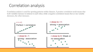
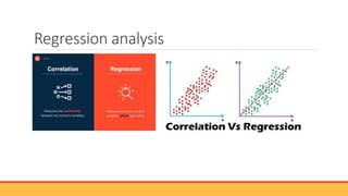
The document explains hypothesis testing in statistics, detailing concepts such as null and alternative hypotheses, significance levels, and p-values. It emphasizes the importance of testing assumptions against data to validate research claims across various fields, including healthcare and education. Additionally, it covers data distribution, correlation analysis, and various statistical tests used to analyze data relationships and differences among groups.

1. Hypothesis testing in
statistics
PREPARED BY MODULE LECTURER M.V.P KARUNARATHE

2. Hypothesis
A hypothesis is a statement or assumption that can be tested by scientific research.
Hypothesis testing ascertains whether a particular assumption is true for the whole population.
A tutoring service claims that its method of tutoring helps 90% of its students get an A or a B.
A company says that women managers in their company earn an average of $60,000 per year.

3. Hypothesis Testing
Or Significance testing.
A formal statistical test called a hypothesis test is used to confirm or disprove a statistical hypothesis.
Hypothesis testing is a statistical interpretation that examines a sample to determine whether the results
stand true for the population.
Why Hypothesis testing
Hypothesis testing helps assess the accuracy of new ideas or theories by testing them against data. This
allows researchers to determine whether the evidence supports their hypothesis, helping to avoid false
claims and conclusions.

4. Types of hypotheses
The test allows two explanations for the data—the null hypothesis or the alternative hypothesis.
Null Hypothesis (H0)
“Null” meaning “nothing.” This hypothesis states that there is no difference between groups or no
relationship between variables. The null hypothesis is a assumption of status or no change.
If the sample mean matches the population mean, the null hypothesis is proven true
Alternative Hypothesis (Ha) – This is also known as the claim. This hypothesis should state what you expect
the data to show, based on your research on the topic. This is your answer to your research question.
If the sample mean is not equal to the population mean, the alternate hypothesis is accepted.

5. Hypotheses testing
H0: The null hypothesis:
Ha: The alternative
There are two options for a decision. They are
"reject H0" if the sample information favors the alternative hypothesis or
"do not reject H0" or "decline to reject H0" if the sample information is insufficient to reject the null hypothesis.

6. Examples

7. Example
Null Hypothesis: H0: There is no difference in the salary of factory workers based on gender.
Alternative Hypothesis: Ha: Male factory workers have a higher salary than female factory workers.
Null Hypothesis: H0: There is no relationship between height and shoe size.
Alternative Hypothesis: Ha: There is a positive relationship between height and shoe size.
Null Hypothesis: H0: Experience on the job has no impact on the quality of a brick mason’s work.
Alternative Hypothesis: Ha: The quality of a brick mason’s work is influenced by on-the-job
experience.

8. Simple hypothesis
In a simple hypothesis, the population parameter is stated as a specific value, making the analysis
easier.
example
We want to test whether the mean GPA of students in ABC institute is different from 2.0 (out of
4.0). The null and alternative hypotheses are:
H0:μ=2.0
Ha:μ≠2.0

9. Real-World Examples
Healthcare
In the healthcare industry, all the research and experiments which are done to predict the
success of any medicine or drug are done successfully with the help of Hypothesis testing.
Education sector
Hypothesis testing assists in experimenting with different teaching techniques to deal with the
understanding capability of different students
Mental Health
Hypothesis testing helps in indicating the factors that may cause some serious mental health
issues.

10. Data Collection
To prove our statistical test validity, it is essential and critical to check the data and proceed with
sampling them to get the correct hypothesis results.
If the target data is not prepared and ready, it will become difficult to make the predictions or the
statistical inference on the population that we are planning to make.
It is important to prepare efficient data, so that hypothesis findings can be easy to predict

11. Selection of statistical test
Once we get the result and outcome of the statistical test, we have to then proceed further to
decide whether the reject or accept the null hypothesis. The significance level is indicated by alpha
(α).
It describes the probability of rejecting or accepting the null hypothesis. Example- Suppose the
value of the significance level which is alpha is 0.05. Now, this value indicates the difference from
the null hypothesis.

12. Selection of the appropriate significant level
Once we get the result and outcome of the statistical test, we have to then proceed further to
decide whether the reject or accept the null hypothesis.
The significance level is indicated by alpha (α).
It describes the probability of rejecting or accepting the null hypothesis.
Example- Suppose the value of the significance level which is alpha is 0.05. Now, this value
indicates the difference from the null hypothesis.

13. Significance Level (Alpha)
The significance level, also known as alpha or α, is an evidentiary standard that researchers set before
the study. It specifies how strongly the sample evidence must contradict the null hypothesis before
you can reject the null for the entire population.
In a hypothesis test, the p value is compared to the significance level to decide whether to reject the
null hypothesis.
If the p value is higher than the significance level, the null hypothesis is not disproved, and the
results are not statistically significant.
If the p value is lower than the significance level, the results are interpreted as disproving the null
hypothesis and reported as statistically significant.

14. P-value
P-value Definition
The P-value is known as the probability value. It is defined as the probability of getting a result
that is either the same or more extreme than the actual observations.
P-value Decision
P-value > 0.05
The result is not statistically significant and hence
don’t reject the null hypothesis.
P-value < 0.05
The result is statistically significant. Generally,
reject the null hypothesis in favour of the
alternative hypothesis.
P-value < 0.01
The result is highly statistically significant, and thus
rejects the null hypothesis in favour of the
alternative hypothesis.

15. P-value
When the p-value is sufficiently small (e.g., 5% or less), then the results are not easily explained by
chance alone and the null hypothesis can be rejected.
When the p-value is large, then the results in the data are explainable by chance alone, and the data is
deemed consistent with (while proving) the null hypothesis.
A small p (≤ 0.05), reject null hypothesis. This is strong evidence that the null hypothesis is
invalid.
A large p (> 0.05) means the alternate hypothesis is weak, so you do not reject the null.

16. P-value

17. Findings of the test
After knowing the P-value and statistical significance, we can determine our results and
take the appropriate decision of whether to accept or reject the null hypothesis based on
the facts and statistics presented to us.

18. Data distribution
Distributions are considered to be any population that has a scattering of data. It’s important to
determine the population’s distribution so we can apply the correct statistical methods when
analyzing it.
Data distributions are widely used in statistics. Suppose an engineer collects 500 data points on a
shop floor. It does not give any value to the management unless they categorize or organize the
data in a useful way. Data distribution methods organize the raw data into graphical methods like
histograms, box plots and provide helpful information.

19. Data distribution
Data can be "distributed" (spread out) in different ways.
Spread-out more to left More to right

20. Data distribution

21. Symmetrical distribution
symmetrical distribution appears as a bell curve. The perfect normal distribution is the
probability distribution that has zero skewness.
Example: High school students weigh between 80lbs and 100lbs, and the majority of students
weigh around 90lbs.
The weights are equally distributed on both sides of 90 lbs, which is the center value.

22. Positively Skewed Distribution
We say that a distribution skews to the right if it has a long tail that trails toward the right side. The
skewness value of a positively skewed distribution is greater than zero.
The income details of the Chicago manufacturing employees indicate that most people earn
between $20K and $50K per annum. Very few earn less than $10K, and very few earn $100K. The
center value is $50K. It is very clear from the graph a long tail is on the right side of the center
value.

23. Negatively Skewed Distribution
Distribution is said to be skewed to the left if it has a long tail that trails toward the left side. The
skewness value of a negatively skewed distribution is less than zero.
A professor collected students’ marks in a science subject. The majority of students score
between 50 and 80, while the center value is 50 marks. The long tail is on the left side of the
center value because it is skewed to the left-hand side of the center value. So the data is
negative skew distribution.

24. What Is a Normal Distribution
Normal distribution, also known as the Gaussian distribution, is a probability distribution that is symmetric about the
mean, showing that data near the mean are more frequent in occurrence than data far from the mean. The frequency
sharply decreases as values are away from the central value on either side.
The resultant graph appears as bell-shaped where the mean, median, and mode are of the same values and appear at
the peak of the curve.
The normal distribution has several key features
First, its mean (average), median (midpoint), and mode (most frequent observation) are all equal to one another.

25. Normal Distribution

26. Empirical Rule
Data will fit within three standard deviations of the mean!

27. Example
Average academic performance of all the students

28. Example
Birthweight of Babies
the birthweight of newborn babies is normally distributed with a mean of about 7.5 pounds.
The histogram of the birthweight of newborn babies in the U.S. displays a bell-shape that is typically
of the normal distribution

29. Parametric and non-parametric
Conducting statistical hypothesis tests.
A very common requirement is that the data used must be subject to some distribution, usually
the normal distribution If your data are normally distributed, parametric tests can usually be used, if
they are not normally distributed, non-parametric tests are usually used.

30. Contd

31. Normality test
A normality test determines whether a sample data has been drawn from a normally distributed
population.
It is generally performed to verify whether the data involved in the research have a normal distribution.
Graphical Method of Assessing Normality
The most useful method of visualizing the normality distribution of a certain variable is to plot the data
on a graph called as a frequency distribution chart or histogram.

32. Analytical Method of Assessing Normality
Shapiro-Wilks test. This test tests the null hypothesis that a sample is drawn from a normal
distribution.
Anderson-Darling test, which is more sensitive to deviations from normality in the distribution’s tails.
The Kolmogorov-Smirnov test compares the sample distribution to a normal one with the same
mean and standard deviation.

33. Shapiro-Wilk normality test
Shapiro test is a statistical test used to check whether the considered data is normally distributed data
or not.
The null hypothesis is states that the population is normally distributed
i.e if the p-value is greater than 0.05, then the null hypothesis is accepted.
The alternative hypothesis states that the population is not normally distributed i.e if the p-value is
less than or equal to 0.05, then the null hypothesis is rejected

34. One-sample t test
One-sample t-test is used to compare the mean of one sample to a known
standard mean (μ).
The t tests are based on an assumption
◦ data come from the Normal distribution, The data are continuous (not discrete), The sample is a simple
random sample from its population. Each individual in the population has an equal probability of being
selected in the sample.
Example
weights <- c(301, 305, 312, 315, 318, 319, 310, 318, 305, 313, 305, 305, 305)
t.test(x = weights, mu = 310)

35. Two-sample t test
The two-sample t test is used to test the hypothesis that two samples may be assumed to come from
distributions with the same mean.
Notice that the necessary information is contained in two parallel columns of a data frame
group1 <- c(8, 8, 9, 9, 9, 11, 12, 13, 13, 14, 15, 19)
group2 <- c(11, 12, 13, 13, 14, 14, 14, 15, 16, 18, 18, 19)
t.test(group1, group2, var.equal=TRUE)

36. Example
Body weight among boys and girls in class are known to be normally distributed, each with
sample standard deviations for girls is 25 and for boys is 23.
A teacher wants to know if the mean body weight between girls and boys in class are different,
so she selects two random samples of boys and girls each of size 20 from the class and records
their weights.

37. Correlation analysis
Correlation analysis is used for spotting patterns within datasets. A positive correlation result means that
both variables increase in relation to each other, while a negative correlation means that as one variable
decreases, the other increases.

38. Correlation coefficient
If the correlation coefficient is close to 1, it would indicate that the variables are positively
linearly related and the scatter plot falls almost along a straight line with positive slope.
For -1, it indicates that the variables are negatively linearly related and the scatter plot
almost falls along a straight line with negative slope.
And for z
-1 indicates a strong negative correlation : this means that every time x increases, y
decreases
0 means that there is no association between the two variables (x and y
1 indicates a strong positive correlation : this means that y increases with x Zero, it
would indicate a weak linear relationship between the variables.

39. Pearson's correlation
Parametric correlation test because it depends on the distribution of the data.
Pearson's correlation test measures relations between two quantitative continues variables that have a
linear relationship
Its value ranges from -1 to +1, with 0 denoting no linear correlation, -1 denoting a perfect negative
linear correlation, and +1 denoting a perfect positive linear correlation
set.seed(150)
data <- data.frame(x = rnorm(50, mean = 50, sd = 10),
random = sample(c(-10:10), 50, replace = TRUE))
data$y <- data$x + data$random
correlation <- cor(data$x, data$y, method = 'pearson')

40. Analysis of Variance(ANOVA)
An ANOVA (“Analysis of Variance”) is a statistical technique that is used to determine
whether or not there is a significant difference between the means of three or more
independent groups. The two most common types of ANOVAs are the one-way ANOVA
and two-way ANOVA.
in using ANOVA the relationship between an independent variable and one quantitative
dependent variable.
EX:comparing the sales performance of different stores in a retail chain.

41. Regression analysis

42. Simple linear regression
We consider situations where you want to describe the relation between two variables
using linear regression analysis. Example:short.velocity as a function of blood.glucose.

43. Links to refer
https://www.youtube.com/watch?v=ENMseuPQcdA
https://www.youtube.com/watch?v=66z_MRwtFJM
https://www.tutorialspoint.com/r/index.htm https://slideplayer.com/slide/14548486/
https://www.scribbr.com/statistics/pearson-correlation-coefficient/
https://www.youtube.com/watch?v=RlhnNbPZC0A
https://www.youtube.com/watch?v=kvmSAXhX9Hs
https://www.youtube.com/watch?v=fT2No3Io72g
https://www.youtube.com/watch?v=0m-rs2M7K-Y