I gave this talk at the Cesium Developer Conference 2025 in philadelphia. In this talk, I've shared my company's experiences of visualizing spatio-temporal data (e.g., chemical dispersion, atmospheric data, wind patterns, and water flow) using CesiumJS. While CesiumJS excels at rendering massive, heterogeneous 3D objects, visualizing spatio-temporal data remains challenging due to its dynamic nature. To address these challenges, we explored workaround solutions to efficiently handle and visualize large-scale spatio-temporal data, aiming for intuitive representation and realistic simulation. As a result, we successfully developed techniques for chemical dispersion visualization, water flow simulation, and atmospheric data rendering over time.

1. Acknowledgement: This work was supported by Korea Environment Industry & Technology Institute (KEITI) through
'Advanced Technology Development Project for Predicting and Preventing Chemical Accidents' program.
How to Visualize the
Spatio-Temporal Data Using CesiumJS
Jinho Kim, Yongsub Kwak, Jinhoon Kim, Sanghee Shin
Gaia3D, Inc.

2. Introduction
1. Weather Data Visualization
2. Visualizing Chemical Dispersion
3. Fluid Simulation & Visualization
Q & A
Contents
2

3. Introduction
How to Visualize the Spatio-Temporal Data Using CesiumJS
3
Weather Data Visualization Fluid Simulation & Visualization
Spatio-Temporal Visualization of Chemical
Dispersion
We have conducted various projects focused on visualizing spatio-temporal data including environmental impact
assessments, chemical accident risk assessments, and meteorological data visualization.
Initially, we developed our own JavaScript library called mago3D.JS for rendering these datasets. However, in line
with 3D GIS standards and the broader ecosystem, we now carry out most of our projects using CesiumJS.

4. 4
1. Weather Data Visualization
Acknowledgement: Much of this work was funded by the Korea
Meteorological Administration (KMA) for the development of a w
eb-based 3D visualization system for numerical weather predicti
on models.

5. Weather Data Visualization
Weather Data Visualization
Our first case study focuses on visualizing numerical weather prediction models. Much of this work was sponsored by
the Korea Meteorological Administration (KMA).
• Visualizing iso-value surface of weather variables
• Visualizing streamline data like wind flows
• Visualizing slice plots of 3D volume
Animated wind flows
Iso-surface of wind speed over
50m/s
Slice plots of wind speed
5

6. Weather Data Pre-processing
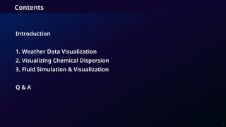
Weather Data Visualization
• Meteorological data is distributed in a grid data format with multiple isobaric pressure levels and weather variables
(points : ~10M ).
• The data is pre-generated on the backend.
• There are many forecast models(ECMWF, GFS, KIM) and visualization methods.
• Each forecast model uses different grid definitions, map projections.
• To reduce complexity, we use unified grid data format which is applicable in both 2D, 3D spatial operation.
Unified Grid format
(lon,lat,alt,value)[]
ECMWF
KIM
Iso-surface
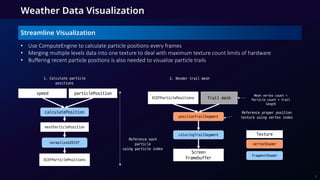
Streamline
Weather forecast models Visualization methods
6

7. Iso-surface Visualization
We use iso-surfaces to represent areas of constant values. This is effective for visualizing volumetric data like
temperature, pressure, or cloud density.
1. Make iso-surface meshes in GLTF format using marching cube algorithms.
2. Vertex position transformation : Index coordinates => lon, lat, alt => ECEF coordinates
3. Using standard atmosphere pressure-altitude table to convert pressure levels to real altitudes.
Weather Data Visualization
1. Marching cube in grid index
space
2. Convert vertex positions to ECEF coordinates 3. Calculate normal from ECEF
coordinates
7

8. Streamline Visualization
To visualize vector fields like wind, we use streamlines. This technique clearly shows the direction and velocity of wind
patterns over large geographical areas.
• Animated streamline in 3D space to visualize velocity vector field like wind speed
• Calculate and render each particles using Cesium Compute Engine + CustomShader
• Inspired by GPU Powered Wind Visualization With Cesium – Cesium
Weather Data Visualization
8

9. Streamline Visualization
• Use ComputeEngine to calculate particle positions every frames
• Merging multiple levels data into one texture to deal with maximum texture count limits of hardware
• Buffering recent particle positions is also needed to visualize particle trails
Weather Data Visualization
speed particlePosition
nextParticlePosition
normalized2ECEF vertexShader
fragmentShader
calculatePosition
ECEFParticlePositions
Reference each
particle
using particle index
positionTrailSegment
coloringTrailSegment
1. Calculate particle
positions
ECEFParticlePositions
2. Render trail mesh
Screen
Framebuffer
Trail mesh
Mesh vertex count =
Particle count * trail
length
Reference proper position
texture using vertex index
Texture
9

10. Slice Plots
Slice plots allow us to render a 2D cross-section of the 3D data. This is useful for analyzing the data at a specific
altitude or plane.
• Slice plots also can help to visualize 3D grid data
• Render a mesh with 3 generated planes and for each axis calculates proper ECEF coordinates
Weather Data Visualization
10

11. 3D Visualization System for Numerical Prediction Models - KMA
Weather Data Visualization
11

12. 12
2. Visualizing Chemical Dispersion

13. Next, we'll demonstrate how we visualize chemical dispersion simulations. This system is designed to predict and
display the spread of hazardous materials in an urban environment following an accident.
• Data converting & reducing
• Data interpolation & volume rendering
Overview
13
Visualizing Chemical Dispersion

14. Visualizing Chemical Dispersion
environmental
dynamicmodel
Concentration
value
PNG
value coding (32GB -> 0.16GB)
• Challenge: The raw simulation data is extremely large, often over 30GB, which is too big to transfer and
render in a web browser.
• Solution 1(Data Encoding): We encode the concentration values into the RGBA channels of PNG images.
This significantly compresses the data size, in this case from 32GB down to just 160MB.
• Solution 2(Client-side Interpolation): Instead of sending every single time step, we only send keyframes. The
client then generates the frames in between using linear interpolation for smother animation.
Tackling the Problems - Optimization of Model Data
14

15. Visualizing Chemical Dispersion
Our visualization is based on a volume rendering technique using ray casting. The process for each pixel is:
1. Ray Casting: A ray is cast from the camera through the pixel into the data volume.
2. Sampling: Data values are sampled at intervals along the ray.
3. Shading: Lighting and color are applied to the sampled points.
4. Compositing: The shaded samples are blended together to calculate the final pixel color.
One pixel in an image
Model
Data
Area
Image to be displayed
on monitor
Volume Rendering
15
1.Raycasting 2.sampling 3.shading 4.compositing

16. • Exploring varied visualization of chemical concentrations by adjusting rendering parameters such as color
mapping and opacity.
• Expanded profiling capabilities for plane slicing, enabling detailed analysis and quantitative inspection on cross-
sections.
• Combining volume rendering and profiling enables comprehensive investigation of the spatio-temporal
evolution of chemical dispersion.
Volume Rendering Result
Visualization of chemical concentration
volumes sliced into a plane.
Visualizing Chemical Dispersion
Volume Rendering Result and Extension
16

17. Visualizing Chemical Dispersion
Research progress - 1st Year
17

18. Visualizing Chemical Dispersion
Research progress - 2nd Year
18

19. Visualizing Chemical Dispersion
Research progress - 3rd Year (Current)
19
• This year, we are developing and working on visualizing both VolumeRender and Isosurface using the Marching
Cube algorithm developed for KMA.

20. 20
3. Fluid Simulation & Visualization

21. Fluid Simulation & Visualization
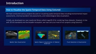
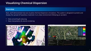
Overview
We explored two approaches: real-time simulation and pre-computed simulation.
1. Real-time allows for live interaction but can be slow and requires a powerful client.
2. Pre-computed is much faster for rendering and allows you to scroll back and forth in time, but it requires high
memory and significant network traffic upfront. It does not support live interaction.
[Water generation from water source] [Precipitation control]
21

22. Precomputed
Real-time
Fluid Simulation & Visualization
Simulation & Visualization
• Separate development of Simulation and Visualization.
• We've developed a real-time water simulation that runs in the browser, along with separate visualization
techniques for precomputed simulations.
22

23. Fluid Simulation & Visualization
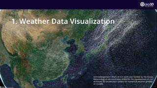
Realtime Simulation VS Precomputed Simulation
• Realtime processing is simulation using GPUs to allow real-time interaction, but client performance is critical,
browser stability is an issue, and complex simulations are difficult.
• Precomputed processing is smooth because you only need to visualize the pre-calculated results. However, as
the resolution of simulations increases, streaming data lightweighting technologies become more important.
[Control time through scrolling]
[Realtime and Precomputed Comparisons]
Compare Realtime Precomputed
Live Interaction Enabled Disabled
Network Traffic no High
Rendering Speed Slow Fast
Memory Usage low High
Time Flow One-Way Two-way
23

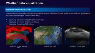
24. Types of Fluid Visualization Methods
There are several methods for visualizing fluids. We explored three main types:
1. Grid-Based: Such as the Height-Field or Height Map method.
2. Particle-Based: Using techniques like Smoothed-Particle Hydrodynamics (SPH).
3. Volume-Based: Using algorithms like Marching Cubes to generate a mesh from the volume.
[Particle Based Visualization]
SPH(Smoothed-particle hydrodynamics)
[Grid Based Visualization]
Height-Field/Height Map
[Volume Based Visualization]
(Marching Cube / Dual Contouring)
24
Fluid Simulation & Visualization

25. Height-Field Visualization Method
We chose the Height-Field method for its performance. It works by taking a simple 2D grid mesh and displacing its
vertices up or down based on the color values in a 'water height' texture. This efficiently creates the appearance of
a 3D water surface.
4.0 3.0
3.0 2.0
2.0
1.0
1.0
0.0
2.0 1.0
1.0 0.0
0.0
0.0
0.0
0.0
Water Height Texture
(4x4, png)
Grid Mesh
(4x4, gltf)
Grid Mapping Above View Create depth
through height texture
25
Fluid Simulation & Visualization

26. Height-Field Visualization Method - Similar cases
• This technique is quite popular and is used in well-known WebGL demos like Evan Wallace's 'WebGL Water'. These
simulations use a height-field for the water surface and then add advanced effects like ray-traced reflections,
refractions, and caustics for realism.
[WebGL Water Page ScreenShot]
26
Fluid Simulation & Visualization

27. Height-Field Visualization Method
• Results of visualization of implemented simulation as wireframe
27
[Visualized as wireframe]
Fluid Simulation & Visualization

28. Simulation Method
• The in-house developed simulation is a lattice-based simulation using SWE, which can be discretized into a 2D
lattice with equations derived from NSE, enabling calculations using GPUs, and is suitable for large-scale terrain-
based water flows such as floods.
• Other CFD programs would have been similar. but would have had different policies for calibrating the
simulation, such as handling boundary conditions.
Comparison Complexity Applicability Application Areas
NSE (Navier-Stokes Equatio
ns)
Very Complex
Applicable to all fluid
s
Most areas of CFD, aerospace,
meteorology, fluids, etc.
SWE (Shallow Water Equatio
ns)
Simple
Applicable to shallow w
ater
Shallow water, tsunamis,
flood modeling, ocean tides,
river flows
[Comparison table]
[Wikipedia’s SWE Image]
28
Fluid Simulation & Visualization

29. Conclusion
With structured visualization methods and formats, and a hybrid of real-time and batch approaches, we can integra
te with external CFD modules while offering lightweight, web-based visualizations.
By combining a height-field simulation with Cesium's 3D globe, we can create compelling and interactive visualizati
ons of fluid dynamics. This is highly effective for applications like urban flood simulation or analyzing water flow ove
r natural terrain.
29
Fluid Simulation & Visualization

30. Q&A
30

31. Thank you!
Web: www.gaia3d.com
YouTube: https://www.youtube.com/@mago3d890
Facebook: https://www.facebook.com/Gaia3d
X(Twitter): https://twitter.com/Gaia3D
Github: https://github.com/Gaia3D
31