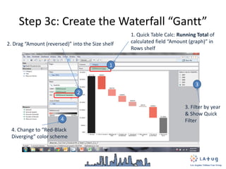
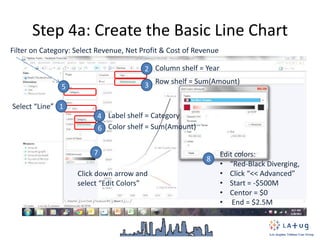
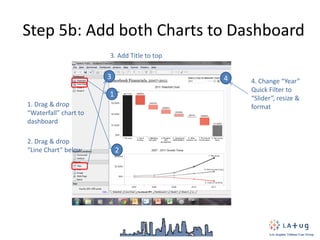
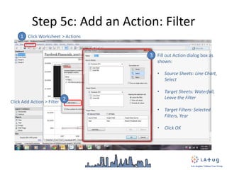
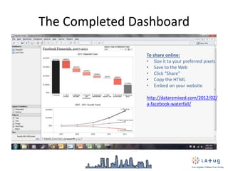
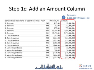
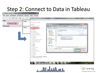
The document provides a step-by-step guide for creating a waterfall chart in Tableau based on Facebook's income statement data. It includes instructions for data preparation in Excel, connecting to Tableau, creating Gantt and line charts, and assembling a dashboard with interactive features. Key techniques like calculated fields, dual axis charts, and synchronization are outlined to transform financial data into a visual dashboard.

1. How to Make a Waterfall Chart in
Tableau

2. A Business Dashboard Challenge:
• Turn an income statement into an
interactive dashboard:
(Facebook IPO Form S-1 from SEC Edgar website)
http://dataremixed.com/2012/02/a-facebook-waterfall/

3. Step 1a: Get the Data
• Financials from SEC website copy/pasted into
Excel table:
ConsolidatedStatements of Operations Data: 2 0 0 7 2 0 0 8 2 0 0 9 2 0 10 2 0 11
1. Revenue $ 153 $ 272 $ 777 $ 1,974 $ 3,711
2. Cost of revenue $ (41) $ (124) $ (223) $ (493) $ (860)
3. Marketing and sales $ (32) $ (76) $ (115) $ (184) $ (427)
4. Research and development $ (81) $ (47) $ (87) $ (144) $ (388)
5. General and administrative $ (123) $ (80) $ (90) $ (121) $ (280)
6. Other expense, net $ (11) $ (1) $ (8) $ (24) $ (61)
7. Provision for income taxes $ (3) $ - $ (25) $ (402) $ (695)
8. Net income (loss) $ (138) $ (56) $ 229 $ 606 $ 1,000

4. Step 1b: Reshape the Data in Excel
http://kb.tableausoftware.com/articles/knowledgebase/addin-reshaping-data-excel
https://www.interworks.com/blogs/tcostello/2012/02/06/preparing-data-tableau-1-3-video-tutorial
1
2
3
4

5. Step 1c: Add an Amount Column
Consolidated Statements of Operations Data: Year Amount_mil Amount
1. Revenue 2007 $153.00 153,000,000
1. Revenue 2008 $272.00 272,000,000
1. Revenue 2009 $777.00 777,000,000
1. Revenue 2010 $1,974.00 1,974,000,000
1. Revenue 2011 $3,711.00 3,711,000,000
2. Cost of revenue 2007 ($41.00) (41,000,000)
2. Cost of revenue 2008 ($124.00) (124,000,000)
2. Cost of revenue 2009 ($223.00) (223,000,000)
2. Cost of revenue 2010 ($493.00) (493,000,000)
2. Cost of revenue 2011 ($860.00) (860,000,000)
3. Marketing and sales 2007 ($32.00) (32,000,000)
3. Marketing and sales 2008 ($76.00) (76,000,000)
3. Marketing and sales 2009 ($115.00) (115,000,000)
3. Marketing and sales 2010 ($184.00) (184,000,000)
3. Marketing and sales 2011 ($427.00) (427,000,000)
1
Amount =
1,000,000*Amount_mil

6. Step 2: Connect to Data in Tableau

7. Step 3a: Begin a Gantt Bar Chart
2 Drag “Category” to the Columns shelf
1 Select “Gantt Bar” chart

8. Step 3b: Create Two Calculated Fields
1 Right click anywhere in the “Measures” area and select “Create Calculated Field
2 “Amount (graph)”:
IF Category="8. Net income
(loss)" THEN [Amount]*-1 ELSE
[Amount] END
3 “Amount (reversed)”:
[Amount (graph)]*-1

9. Step 3c: Create the Waterfall “Gantt”
1
2
1. Quick Table Calc: Running Total of
calculated field “Amount (graph)” in
Rows shelf
2. Drag “Amount (reversed)” into the Size shelf
3
3. Filter by year
& Show Quick
Filter4
4. Change to “Red-Black
Diverging” color scheme

10. Step 4a: Create the Basic Line Chart
2
1
3
4
5
6
7
8
Column shelf = Year
Row shelf = Sum(Amount)
Select “Line”
Label shelf = Category
Filter on Category: Select Revenue, Net Profit & Cost of Revenue
Edit colors:
• “Red-Black Diverging,
• Click “<< Advanced”
• Start = -$500M
• Centor = $0
• End = $2.5M
• Click “OK”
Color shelf = Sum(Amount)
Click down arrow and
select “Edit Colors”

11. Step 4b: Create a “Dual Axis”,
“Multiple Mark Type” chart
1 Hold down “Ctrl”, left click on SUM(Amount) in the Row shelf, and drag & drop to
the right to add a second SUM(Amount) to the Row shelf
2
3
Click down arrow in 2nd
SUM(Amount) and select
“Dual Axis”
Click down arrow in
Marks area and select
“Multiple Mark Types”

12. Step 4b: Synchronize Axis
1
2
Right click 2nd Y-axis and
select “Synchronize Axis”
Uncheck “Show Header”

13. Step 4c: Make 2nd Mark Type Circles
1
2
3
Click right (“>”) until “SUM(Amount) (2)” is showing
Change the type from “Line” to “Circle” and reduce the
size of the circles by dragging the “Size” slider to the left
3. Click on the “Label” down arrow and
uncheck “Show mark labels” to clean up
the chart

14. Step 5a: Create a New Dashboard
1
Right click on the new tab icon
and select “New Dashboard”

15. Step 5b: Add both Charts to Dashboard
3
3. Add Title to top
4 4. Change “Year”
Quick Filter to
“Slider”, resize &
format
1
1. Drag & drop
“Waterfall” chart to
dashboard
2
2. Drag & drop
“Line Chart” below

16. Step 5c: Add an Action: Filter
1 Click Worksheet > Actions
2Click Add Action > Filter
3 Fill out Action dialog box as
shown:
• Source Sheets: Line Chart,
Select
• Target Sheets: Waterfall,
Leave the Filter
• Target Filters: Selected
Filters, Year
• Click OK

17. The Completed Dashboard
To share online:
• Size it to your preferred pixels
• Save to the Web
• Click “Share”
• Copy the HTML
• Embed on your website
http://dataremixed.com/2012/02/
a-facebook-waterfall/