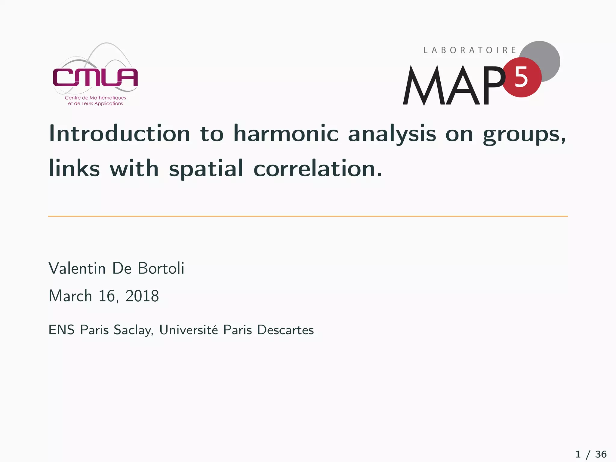
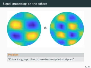
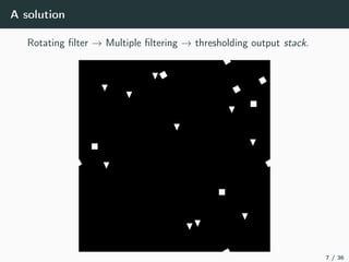
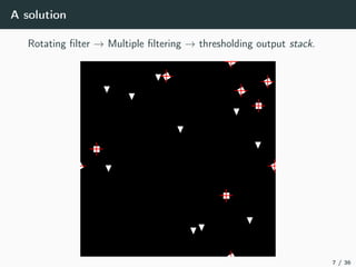
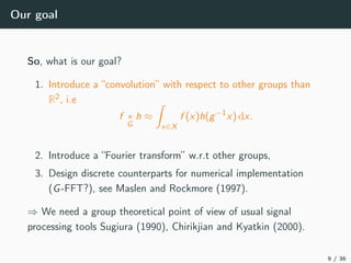
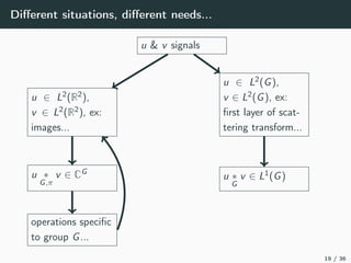
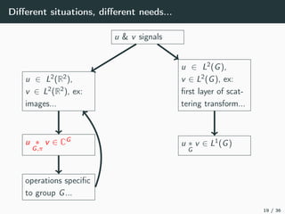
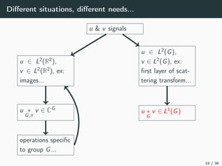
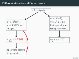
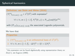
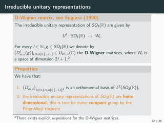
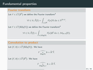
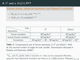
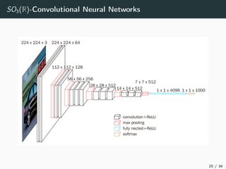
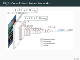
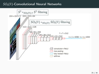
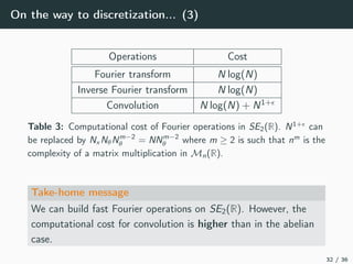
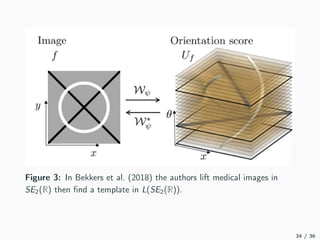
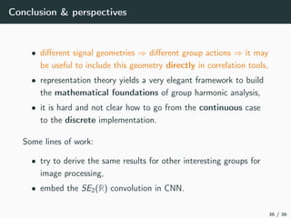
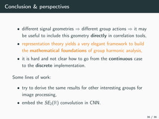
This document introduces harmonic analysis on groups and its connections to spatial correlation. It discusses motivations like defining convolution on the sphere S2. Representation theory provides tools to study this, like spherical harmonics which form an orthonormal basis of L2(S2). Spherical CNNs can be understood through the irreducible unitary representations of SO3(R), which are the Wigner D-matrices. The document explores different types of convolutions defined using representations of a group G, like the G-convolution and the (G,π)-convolution. Wavelet transforms provide a link between these convolutions and representations. The goals are to introduce analogues of convolution and Fourier transforms for general groups beyond R2.


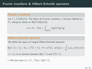
![Link between convolutions
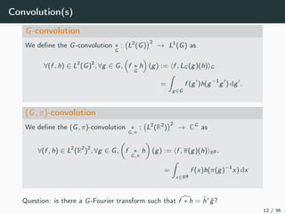
Suppose (π, R2
) is a representation of G.
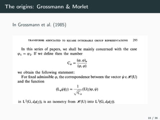
Wavelet Grossmann et al. (1985)
Suppose that π, L2
(R2
) is an irreducible representation of G. Let
ψ ∈ L2
(R2
) a π-admissible vector, i.e g → π(g)(ψ), ψ ∈ L2
(G). Then
W : L2
(R2
) → Im(W) ⊂ L2
(G) defined as
W[f ] =
1
Cψ
π(·)(ψ), f
intertwines π and LG in the sense that
∀g ∈ G, ∀u ∈ L2
(R2
), LG (g)(W[u]) = W[π(g)(u)].
The unitary W operator is called a wavelet transform.
Convolution(s)
Let W be a wavelet transform.
∀(u, v) ∈ L2
(R2
)
2
, u ∗
G,π
v = W[u] ∗
G
W[v].
15 / 36](https://image.slidesharecdn.com/harmonicslide-180319002633/85/Introduction-to-harmonic-analysis-on-groups-links-with-spatial-correlation-22-320.jpg)
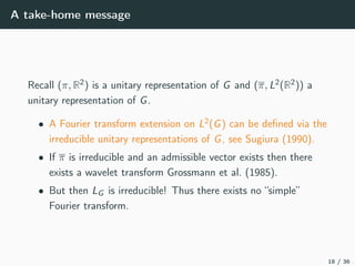
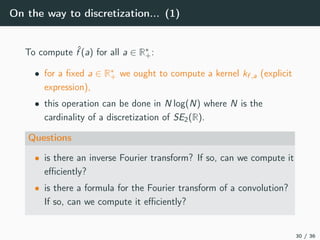
![Summary on wavelets
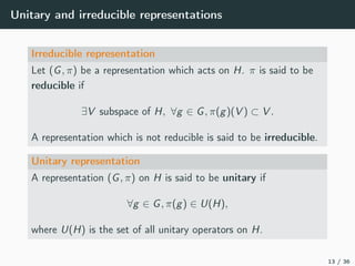
f ∈ L2(R2) π(g)(f ) ∈ L2(R2)
W [f ] ∈ L2(G) W [π(g)(f )] ∈ L2(G)
L2(G)
L2(R2)
space representation
17 / 36](https://image.slidesharecdn.com/harmonicslide-180319002633/85/Introduction-to-harmonic-analysis-on-groups-links-with-spatial-correlation-24-320.jpg)
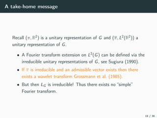
![Summary on wavelets
f ∈ L2(R2) π(g)(f ) ∈ L2(R2)
W [f ] ∈ L2(G) W [π(g)(f )] ∈ L2(G)
L2(G)
L2(R2)
wavelet transform
17 / 36](https://image.slidesharecdn.com/harmonicslide-180319002633/85/Introduction-to-harmonic-analysis-on-groups-links-with-spatial-correlation-25-320.jpg)
![Summary on wavelets
f ∈ L2(R2) π(g)(f ) ∈ L2(R2)
W [f ] ∈ L2(G) W [π(g)(f )] ∈ L2(G)
L2(G)
L2(R2)
wavelet transform
17 / 36](https://image.slidesharecdn.com/harmonicslide-180319002633/85/Introduction-to-harmonic-analysis-on-groups-links-with-spatial-correlation-26-320.jpg)
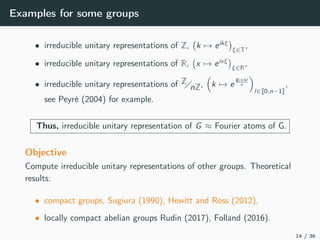
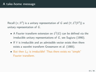
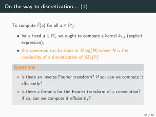
![Summary on wavelets
f ∈ L2(R2) π(g)(f ) ∈ L2(R2)
W [f ] ∈ L2(G) LG (g)(W [f ]) ∈ L2(G)
L2(G)
L2(R2)
regular representation
17 / 36](https://image.slidesharecdn.com/harmonicslide-180319002633/85/Introduction-to-harmonic-analysis-on-groups-links-with-spatial-correlation-27-320.jpg)

 = f (z), → corresponds to set δ0 on L2
(R2
) as an
admissible vector.
2. see Duits et al. (2007) for an extension of wavelets (called
orientation scores) via Reproducing Kernel Hilbert Spaces.
7
This does not imply that no wavelet can be constructed. However it is shown
in Führ (2002) that if there exists an admissible vector on G, with G
unimodular, then G is discrete.
33 / 36](https://image.slidesharecdn.com/harmonicslide-180319002633/85/Introduction-to-harmonic-analysis-on-groups-links-with-spatial-correlation-57-320.jpg)
 = f (z), → corresponds to set δ0 on L2
(R2
) as an
admissible vector.
2. see Duits et al. (2007) for an extension of wavelets (called
orientation scores) via Reproducing Kernel Hilbert Spaces.
7
This does not imply that no wavelet can be constructed. However it is shown
in Führ (2002) that if there exists an admissible vector on G, with G
unimodular, then G is discrete.
33 / 36](https://image.slidesharecdn.com/harmonicslide-180319002633/85/Introduction-to-harmonic-analysis-on-groups-links-with-spatial-correlation-58-320.jpg)
![Working scheme
f ∈ L2(R2) π(g)(f ) ∈ L2(R2)
W [f ] ∈ L2(SE2(R))K W [π(g)(f )] ∈ L2(SE2(R))K
L2(SE2(R))
L2(R2)
space representation
35 / 36](https://image.slidesharecdn.com/harmonicslide-180319002633/85/Introduction-to-harmonic-analysis-on-groups-links-with-spatial-correlation-60-320.jpg)
![Working scheme
f ∈ L2(R2) π(g)(f ) ∈ L2(R2)
W [f ] ∈ L2(SE2(R))K W [π(g)(f )] ∈ L2(SE2(R))K
L2(SE2(R))
L2(R2)
“wavelet” transform
35 / 36](https://image.slidesharecdn.com/harmonicslide-180319002633/85/Introduction-to-harmonic-analysis-on-groups-links-with-spatial-correlation-61-320.jpg)
![Working scheme
f ∈ L2(R2) π(g)(f ) ∈ L2(R2)
W [f ] ∈ L2(SE2(R))K W [π(g)(f )] ∈ L2(SE2(R))K
L2(SE2(R))
L2(R2)
“wavelet” transform
35 / 36](https://image.slidesharecdn.com/harmonicslide-180319002633/85/Introduction-to-harmonic-analysis-on-groups-links-with-spatial-correlation-62-320.jpg)
![Working scheme
f ∈ L2(R2) π(g)(f ) ∈ L2(R2)
W [f ] ∈ L2(SE2(R))K LSE2 (R)(g)(W [f ]) ∈ L2(SE2(R))K
L2(SE2(R))
L2(R2)
regular representation
35 / 36](https://image.slidesharecdn.com/harmonicslide-180319002633/85/Introduction-to-harmonic-analysis-on-groups-links-with-spatial-correlation-63-320.jpg)


![Polymer [ बहुलक ] Chemistry Notes PDF - Irfanullah Mehar - JJ Sir Chemistry.pdf](https://cdn.slidesharecdn.com/ss_thumbnails/polymerchemistrynotespdf-irfanullahmehar-jjsirchemistry-260210172118-3f9b37f7-thumbnail.jpg?width=640&height=640&fit=bounds)


