Download as PDF, PPTX


![Introduction Dynamics of the parabolic problem Numerical results Conclusions
The collision manifold
Regularization of the equations of motion using McGehee’s ideas and
variables to remove one singularity r1 = 0 or r2 = 0 (collision):
x − xmi
= r cos δ v = r1/2
r
y = r sin δ u = r1/2
rδ
ds
dτ
= r3/2
In the regularized equations r = 0 is the collision manifold
There exist two cylinders of equilibrium points:
T±
= {(r, δ, v, u, θ) ∈ R5
| r = 0, v = ±v0, u = 0, δ ∈ [0, 2π], θ ∈ [−π/2, π/2]}
with v0 = 2 (1 − µ).
The unstable (stable) invariant manifold associated to T+
(T−
) is 4
dimensional.
Barrab´es, Cors, Garcia, Oll´e (April 27, 2017) Parabolic problem 15 / 27](https://image.slidesharecdn.com/bmd17parabolic-181120162859/75/Parabolic-Restricted-Three-Body-Problem-18-2048.jpg)


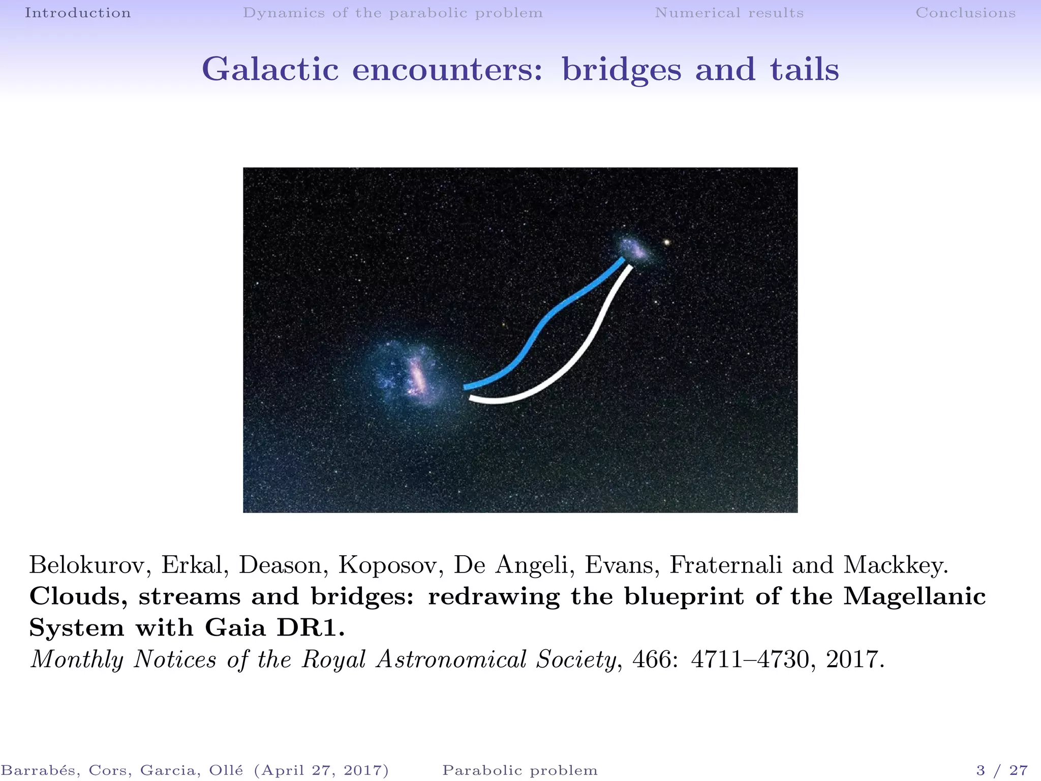
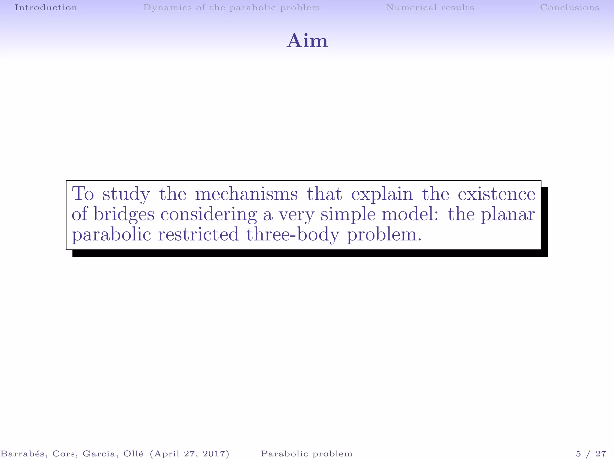
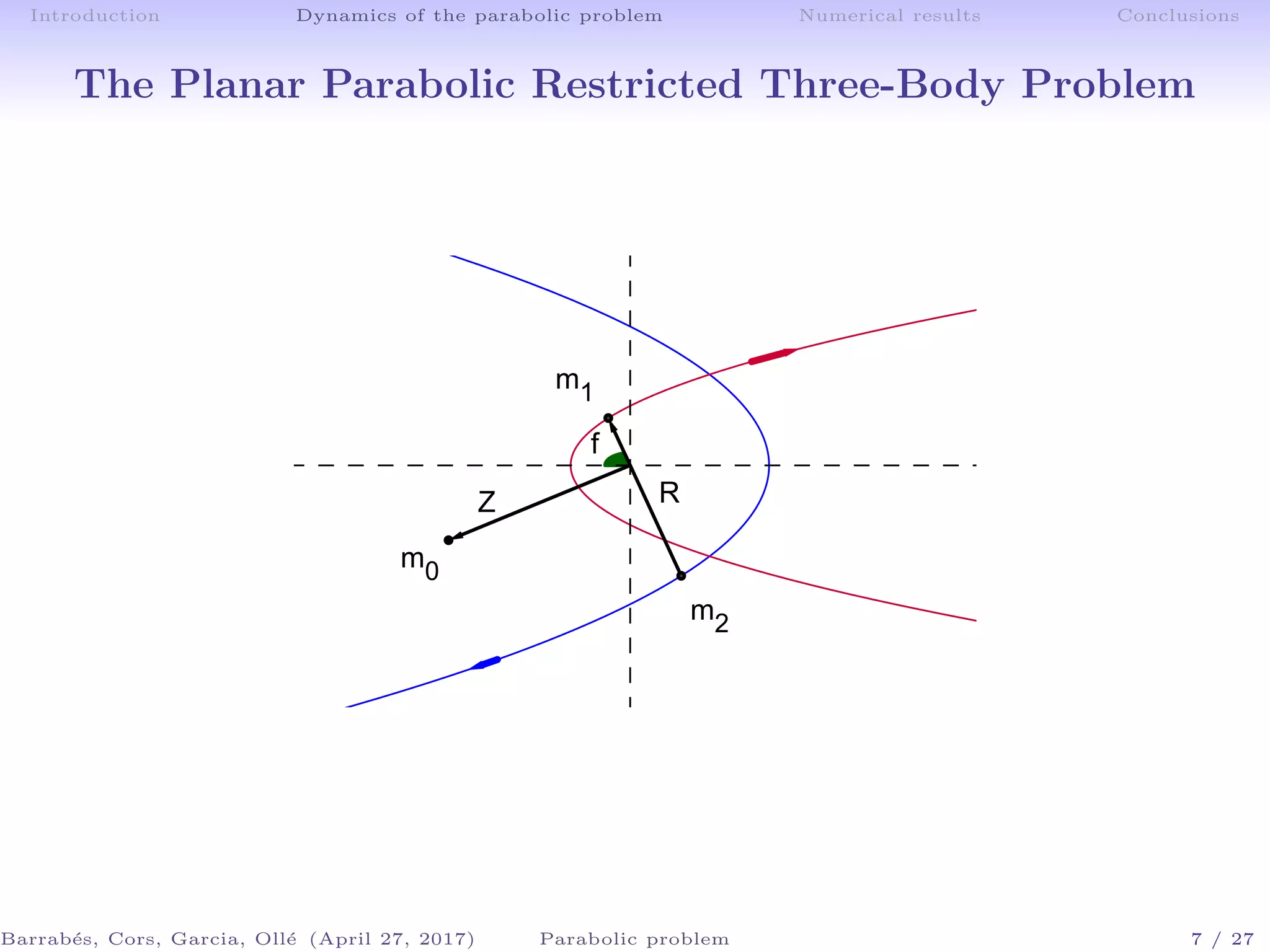
The document discusses the dynamics of galactic encounters using a parabolic restricted three-body problem framework. It examines the conditions that lead to the formation of bridges and tails in galaxies based on numerical simulations and theoretical analyses. Key findings include the identification of equilibrium points and the role of invariant manifolds in determining the outcomes of galactic interactions.