This thesis proposes and evaluates a compressive sensing (CS)-based indoor positioning and tracking system using received signal strength (RSS) from wireless local area network access points. The system is designed and implemented on mobile devices with limited resources. In the offline phase, RSS fingerprints are collected and clustered using affinity propagation. In the online phase, coarse localization is done by matching RSS measurements to precomputed clusters, and fine localization refines the position using CS recovery on the sparse location signal. An indoor tracking system is also presented, which integrates the CS-based positioning with a Kalman filter for sequential location estimates. Experimental results on two testbeds show the system achieves better accuracy than other fingerprinting methods, suitable for implementation

1. RSS-based WLAN Indoor Positioning and Tracking System
Using Compressive Sensing and Its Implementation on
Mobile Devices
by
Anthea Wain Sy Au
A thesis submitted in conformity with the requirements
for the degree of Master of Applied Science
Graduate Department of Electrical and Computer Engineering
University of Toronto
c
Copyright ⃝ 2010 by Anthea Wain Sy Au

2. Abstract
RSS-based WLAN Indoor Positioning and Tracking System Using Compressive Sensing
and Its Implementation on Mobile Devices
Anthea Wain Sy Au
Master of Applied Science
Graduate Department of Electrical and Computer Engineering
University of Toronto
2010
As the demand of indoor Location-Based Services (LBSs) increases, there is a growing interest in developing an accurate indoor positioning and tracking system on mobile
devices. The core location determination problem can be reformulated as a sparse natured problem and thus can be solved by applying the Compressive Sensing (CS) theory.
This thesis proposes a compact received signal strength (RSS) based real-time indoor
positioning and tracking systems using CS theory that can be implemented on personal
digital assistants (PDAs) and smartphones, which are both limited in processing power
and memory compared to laptops. The proposed tracking system, together with a simple
navigation module is implemented on Windows Mobile-operated smart devices and their
performance in different experimental sites are evaluated. Experimental results show
that the proposed system is a lightweight real-time algorithm that performs better than
other traditional fingerprinting methods in terms of accuracy under constraints of limited
processing and memory resources.
ii

3. Acknowledgements
I would like to express my sincere gratitude to my supervisor, Professor Shahrokh Valaee,
whose knowledge, guidance and support have make this work possible. I would also like
to thank Professor Moshe Eizenman, who gives valuable opinions to improve this work.
I owe my special thanks to Chen Feng, whom I have been working with regarding
to this project. In addition, I would like to thank my colleagues at the Wireless and
Internet Research Laboratory (WirLab).
I am grateful for the Natural Sciences and Engineering Research Council of Canada
(NSERC) for its generous financial support.
Finally, I would give my regard to my parents and my sister for their strong moral
supports and encouragement.
iii

4. Contents
1 Introduction
1
1.1
Motivation . . . . . . . . . . . . . . . . . . . . . . . . . . . . . . . . . . .
1
1.2
RSS-based WLAN Positioning Systems . . . . . . . . . . . . . . . . . . .
3
1.2.1
Location-Sensing Techniques . . . . . . . . . . . . . . . . . . . . .
3
1.2.2
Existing Positioning Systems . . . . . . . . . . . . . . . . . . . . .
4
1.3
Problem Statement and Objectives . . . . . . . . . . . . . . . . . . . . .
4
1.4
Technical Challenges . . . . . . . . . . . . . . . . . . . . . . . . . . . . .
6
1.5
Scope
. . . . . . . . . . . . . . . . . . . . . . . . . . . . . . . . . . . . .
8
1.6
Contributions . . . . . . . . . . . . . . . . . . . . . . . . . . . . . . . . .
10
2 Background and Related Works
2.1
12
Signal Propagation Modeling . . . . . . . . . . . . . . . . . . . .
13
2.1.2
Location Fingerprinting . . . . . . . . . . . . . . . . . . . . . . .
14
Fingerprinting-Based Positioning Methods . . . . . . . . . . . . . . . . .
16
2.2.1
K-Nearest Neighbour Method (KNN) . . . . . . . . . . . . . . . .
16
2.2.2
Probabilistic Approach . . . . . . . . . . . . . . . . . . . . . . . .
17
2.2.3
2.3
12
2.1.1
2.2
Indoor RSS-based WLAN Positioning Techniques . . . . . . . . . . . . .
Region of Interest and Access Points Selections . . . . . . . . . .
19
Indoor Tracking . . . . . . . . . . . . . . . . . . . . . . . . . . . . . . . .
21
2.3.1
21
Kalman filter . . . . . . . . . . . . . . . . . . . . . . . . . . . . .
iv

5. 2.3.2
Particle filter . . . . . . . . . . . . . . . . . . . . . . . . . . . . .
21
2.3.3
Other Methods . . . . . . . . . . . . . . . . . . . . . . . . . . . .
22
2.4
Pedestrian Navigation . . . . . . . . . . . . . . . . . . . . . . . . . . . .
23
2.5
Affinity Propagation Algorithm For Clustering . . . . . . . . . . . . . . .
24
2.6
Compressive Sensing Theory . . . . . . . . . . . . . . . . . . . . . . . . .
25
2.7
Chapter Summary . . . . . . . . . . . . . . . . . . . . . . . . . . . . . .
27
3 Compressive Sensing Based Positioning System
28
3.1
Indoor Positioning System Overview . . . . . . . . . . . . . . . . . . . .
28
3.2
Offline Phase . . . . . . . . . . . . . . . . . . . . . . . . . . . . . . . . .
29
3.2.1
Fingerprint Collections . . . . . . . . . . . . . . . . . . . . . . . .
30
3.2.2
Clusters Generation by Affinity Propagation . . . . . . . . . . . .
31
3.2.3
Interaction between the database server and the mobile device during offline phase . . . . . . . . . . . . . . . . . . . . . . . . . . . .
Online Phase . . . . . . . . . . . . . . . . . . . . . . . . . . . . . . . . .
33
3.3.1
Coarse Localization Stage: Cluster Matching . . . . . . . . . . . .
35
3.3.2
Fine Localization Stage: Compressive Sensing Recovery . . . . . .
38
3.3.3
3.3
33
Interaction between the database server and the mobile device during online phase . . . . . . . . . . . . . . . . . . . . . . . . . . . .
3.4
43
Chapter Summary . . . . . . . . . . . . . . . . . . . . . . . . . . . . . .
43
4 Indoor Tracking System
46
4.1
General Bayesian Tracking Model . . . . . . . . . . . . . . . . . . . . . .
47
4.2
Kalman Filter . . . . . . . . . . . . . . . . . . . . . . . . . . . . . . . . .
48
4.3
Overview of Proposed Indoor Tracking System . . . . . . . . . . . . . . .
49
4.3.1
Modified Coarse Localization Stage . . . . . . . . . . . . . . . . .
50
4.3.2
Map-Adaptive Kalman Filter . . . . . . . . . . . . . . . . . . . .
55
Chapter Summary . . . . . . . . . . . . . . . . . . . . . . . . . . . . . .
56
4.4
v

6. 5 Simple Navigation System
59
5.1
Overview of Navigation System . . . . . . . . . . . . . . . . . . . . . . .
59
5.2
Map Database Generation at Initial Setup . . . . . . . . . . . . . . . . .
60
5.2.1
Layout Definition . . . . . . . . . . . . . . . . . . . . . . . . . . .
61
5.2.2
Map Features Definition . . . . . . . . . . . . . . . . . . . . . . .
61
Path Routing Module . . . . . . . . . . . . . . . . . . . . . . . . . . . . .
62
5.3.1
Path Analysis . . . . . . . . . . . . . . . . . . . . . . . . . . . . .
62
Tracking Update Analysis Module . . . . . . . . . . . . . . . . . . . . . .
64
5.4.1
Analysis Process . . . . . . . . . . . . . . . . . . . . . . . . . . .
65
5.4.2
Voice Generation . . . . . . . . . . . . . . . . . . . . . . . . . . .
67
Chapter Summary . . . . . . . . . . . . . . . . . . . . . . . . . . . . . .
68
5.3
5.4
5.5
6 Software Implementation on Mobile Devices
69
6.1
Software Platform . . . . . . . . . . . . . . . . . . . . . . . . . . . . . . .
69
6.2
Devices in Testing . . . . . . . . . . . . . . . . . . . . . . . . . . . . . . .
70
6.3
Software Design . . . . . . . . . . . . . . . . . . . . . . . . . . . . . . . .
72
6.3.1
Software’s Functionalities . . . . . . . . . . . . . . . . . . . . . .
72
6.3.2
Resources Folder . . . . . . . . . . . . . . . . . . . . . . . . . . .
73
6.3.3
Libraries’ Definitions . . . . . . . . . . . . . . . . . . . . . . . . .
74
Chapter Summary . . . . . . . . . . . . . . . . . . . . . . . . . . . . . .
75
6.4
7 Experimental Results
7.1
77
77
7.1.1
Experimental Sites . . . . . . . . . . . . . . . . . . . . . . . . . .
77
7.1.2
Performance Benchmarks . . . . . . . . . . . . . . . . . . . . . . .
81
7.1.3
7.2
Experimental Setup . . . . . . . . . . . . . . . . . . . . . . . . . . . . . .
Figure of Merit . . . . . . . . . . . . . . . . . . . . . . . . . . . .
82
Positioning Results on Bahen Fourth Floor . . . . . . . . . . . . . . . . .
82
7.2.1
82
RSS Distributions . . . . . . . . . . . . . . . . . . . . . . . . . . .
vi

7. 7.2.2
Online Phase: Coarse Localization Analysis . . . . . . . . . . . .
87
7.2.4
Online Phase: Fine Localization Analysis . . . . . . . . . . . . . .
90
7.2.5
Performance Comparison . . . . . . . . . . . . . . . . . . . . . . .
92
Tracking Results on CNIB Second Floor . . . . . . . . . . . . . . . . . .
95
7.3.1
RSS Distributions . . . . . . . . . . . . . . . . . . . . . . . . . . .
96
7.3.2
CS-based Positioning Results . . . . . . . . . . . . . . . . . . . .
96
7.3.3
Modified Coarse Localization Analysis . . . . . . . . . . . . . . .
99
7.3.4
Map Adaptive Kalman Filter Analysis . . . . . . . . . . . . . . . 100
7.3.5
Performance Comparison . . . . . . . . . . . . . . . . . . . . . . . 102
7.3.6
Navigation and Real Time Implementations . . . . . . . . . . . . 104
7.3.7
7.4
85
7.2.3
7.3
Offline Phase: Clustering Results by Affinity Propagation . . . . .
Subject Testing . . . . . . . . . . . . . . . . . . . . . . . . . . . . 106
Chapter Summary . . . . . . . . . . . . . . . . . . . . . . . . . . . . . . 108
8 Conclusion
8.1
109
Future Works . . . . . . . . . . . . . . . . . . . . . . . . . . . . . . . . . 111
Bibliography
113
vii

8. List of Tables
1.1
Existing RSS-based WLAN Position Systems [1] . . . . . . . . . . . . . .
5
1.2
Comparison of a PDA and a laptop . . . . . . . . . . . . . . . . . . . . .
8
6.1
Devices Specifications . . . . . . . . . . . . . . . . . . . . . . . . . . . . .
70
7.1
Comparison of experimental sites . . . . . . . . . . . . . . . . . . . . . .
78
7.2
Traces Summary . . . . . . . . . . . . . . . . . . . . . . . . . . . . . . .
81
7.3
Actual parameters γ (o) used for experiments on Bahen fourth floor. . . .
87
7.4
A set of optimal parameters for the CS-based position system applied on
Bahen fourth floor. . . . . . . . . . . . . . . . . . . . . . . . . . . . . . .
7.5
Position error statistics for different methods on Bahen fourth floor. (For
validation set) . . . . . . . . . . . . . . . . . . . . . . . . . . . . . . . . .
7.6
94
A set of optimal parameters for the CS-based position system applied on
CNIB second floor. . . . . . . . . . . . . . . . . . . . . . . . . . . . . . .
7.8
94
Position error statistics for different methods on Bahen fourth floor. (For
stationary user testing set) . . . . . . . . . . . . . . . . . . . . . . . . . .
7.7
93
99
Positioning error statistics for different positioning methods on CNIB second floor. (For mobile user testing set) . . . . . . . . . . . . . . . . . . . 100
7.9
A set of optimal parameters for the proposed tracking system applied on
CNIB second floor. . . . . . . . . . . . . . . . . . . . . . . . . . . . . . . 103
viii

9. 7.10 Position error statistics for the CS-based positioning system and the two
tracking systems on CNIB second floor. (For mobile user testing set) . . 104
7.11 Summary of the three traces tested by the subjects . . . . . . . . . . . . 107
7.12 Subjects testing results on CNIB second floor . . . . . . . . . . . . . . . 107
ix

10. List of Figures
1.1
The problem setup . . . . . . . . . . . . . . . . . . . . . . . . . . . . . .
6
2.1
Kernel-based method [2]. . . . . . . . . . . . . . . . . . . . . . . . . . . .
20
3.1
Block diagram of the proposed indoor localization system. . . . . . . . .
29
3.2
Interaction between the database server and the mobile device during offline phase.
3.3
. . . . . . . . . . . . . . . . . . . . . . . . . . . . . . . . . .
34
Interaction between the database server and the mobile device during online phase. . . . . . . . . . . . . . . . . . . . . . . . . . . . . . . . . . . .
44
4.1
Block diagram of the proposed indoor tracking system. . . . . . . . . . .
50
4.2
Coarse localization stage for the proposed tracking system. . . . . . . . .
51
4.3
Map-Adoptive Kalman Filter . . . . . . . . . . . . . . . . . . . . . . . .
57
5.1
Navigation System Overview . . . . . . . . . . . . . . . . . . . . . . . . .
60
5.2
Dijkstra Algorithm . . . . . . . . . . . . . . . . . . . . . . . . . . . . . .
63
5.3
Tracking update analysis . . . . . . . . . . . . . . . . . . . . . . . . . . .
64
5.4
A point in close range to a line segment . . . . . . . . . . . . . . . . . . .
65
5.5
Determining the direction of turn based on the two line segments ℓi and ℓi+1 67
6.1
The overview of the software design. Arrows shows the dependency of the
libraries and blue colored boxes are the developed modules for the software. 72
6.2
An example screenshot of Detect AP operation. . . . . . . . . . . . . . .
x
73

11. 7.1
Example histograms of RSS distributions of the same access point over
50 time samples for different devices pointing North at the same reference
point on Bahen fourth floor. . . . . . . . . . . . . . . . . . . . . . . . . .
7.2
84
An example of RSS measurements over time and their averages with respect to the number of time samples of the same access point for different
devices at the same reference point on Bahen fourth floor. . . . . . . . .
7.3
An example of averaged RSS of the same access point in spatial domain
for different orientations and different devices on Bahen fourth floor. . . .
7.4
84
85
Number of clusters generated by the affinity propagation algorithm depending on the value of parameter γ (o) for four orientations on Bahen
fourth floor. . . . . . . . . . . . . . . . . . . . . . . . . . . . . . . . . . .
7.5
86
The clustering results on the four fingerprint databases collected by PDA1
on Bahen fourth floor. Each circle is a RP collected in the database and
each color represents one cluster. . . . . . . . . . . . . . . . . . . . . . .
7.6
The ARMSE versus number of used APs, when different number of generated clusters are used for the coarse localization on Bahen fourth floor .
7.7
89
The cumulative error distributions using different cluster matching schemes
on Bahen fourth floor. (8 APs are used) . . . . . . . . . . . . . . . . . .
7.9
89
The cumulative error distributions using different number of clusters for
the coarse localization on Bahen fourth floor. (8 APs are used) . . . . . .
7.8
88
90
The ARMSE versus number of used APs, using different AP schemes for
fine localization on Bahen fourth floor. . . . . . . . . . . . . . . . . . . .
92
7.10 Effect of the threshold λ1 on ARMSE on Bahen fourth floor. (8 APs are
used) . . . . . . . . . . . . . . . . . . . . . . . . . . . . . . . . . . . . . .
92
7.11 The cumulative error distributions using different positioning systems on
Bahen fourth floor. (8 APs are used) . . . . . . . . . . . . . . . . . . . .
xi
94

12. 7.12 Comparison of mean computation time using different positioning systems
in Bahen fourth floor. (8 APs are used) . . . . . . . . . . . . . . . . . . .
95
7.13 Example histograms of RSS distributions of the same access point over 50
time samples (40 time samples for Smartphone) for different devices at
the same reference point in CNIB second floor. . . . . . . . . . . . . . . .
97
7.14 An example of RSS distributions across time and their averages with respect to the number of time samples of the same access point for different
devices at the same reference point in CNIB second floor. . . . . . . . . .
97
7.15 An example of RSS distributions of the same access point in spatial domain
for different orientations and different devices in CNIB second floor. (only
a part of the fingerprints are shown)
. . . . . . . . . . . . . . . . . . . .
98
7.16 The clustering results on the four fingerprint databases collected by PDA2
on CNIB second floor . . . . . . . . . . . . . . . . . . . . . . . . . . . . .
98
7.17 The cumulative error distributions for different positioning systems on
CNIB second floor. (10 APs are used) . . . . . . . . . . . . . . . . . . . .
99
7.18 Effect of the walking distance β on ARMSE in CNIB second floor. (10
APs are used) . . . . . . . . . . . . . . . . . . . . . . . . . . . . . . . . . 101
7.19 The cumulative error distributions using different Kalman filter parameters in CNIB second floor. (10 APs are used) . . . . . . . . . . . . . . . . 101
7.20 The cumulative error distributions for different Kalman filter update schemes
in CNIB second floor. (10 APs are used) . . . . . . . . . . . . . . . . . . 102
7.21 The cumulative error distributions using the CS-based positioning system
and the three tracking systems in CNIB second floor. (10 APs are used) . 103
7.22 Example trace results. The black line is the actual trace, the green dots
are the CS-based positioning results and the purple line is the results of
the proposed tracking system. . . . . . . . . . . . . . . . . . . . . . . . . 104
xii

13. 7.23 The definition of the connected graph and the map features on CNIB
second floor. The blue lines and blue circles represent the edges and nodes
of the connected graph. The red squares represents the destinations. The
diamonds represents the map features and the pink circles represents the
locations of the 15 deployed access points . . . . . . . . . . . . . . . . . . 105
7.24 Example screenshot of the software that shows the actual track that the
user is walking. The line shows the routed path generated by the navigation module. The squares denote the user’s locations and the circle
denotes the destination. . . . . . . . . . . . . . . . . . . . . . . . . . . . 106
xiii

14. Chapter 1
Introduction
1.1
Motivation
With the wide deployment of the mobile wireless systems and networks, the locationbased services (LBSs) are made possible on mobile devices, such as laptops, smartphones
and personal digital assistants (PDAs). There are a lot of applications that rely on the
locations of these mobile devices, such as navigation, people and assets tracking, locationbased security and coordination of emergency and maintenance responses to accidents,
interruptions of essential services and disasters, etc [3–5].
In order to deliver reliable LBSs, real-time and accurate user’s locations must be obtained. Hence, there is a growing interest in developing effective positioning and tracking
systems. For the outdoor environment, Global Positioning System (GPS) and cellular
network based systems [3,6,7] are commonly used as the techniques to provide navigation
services. However, these techniques cannot be used directly in indoors, as the signals are
usually too weak to be used for localization purposes. Thus, wireless indoor positioning
has become an increasingly popular research topic in recent years.
There are several methods that are built on top of the GPS-capable phones to provide
indoor localization [8]. One example is the Assisted GPS (A-GPS), which requires a
1

15. Chapter 1. Introduction
2
connection to a network location server in order to obtain the estimated location with
an average of 5-50m accuracy [8]. Another one is the Calibree proposed in [9], which
utilizes the detected signal strength from GSM cell towers to determine relative positions
of mobile phones and their absolute locations can be determined if some of the phones are
equipped with GPS receivers. In addition, indoor localization can also be implemented
on GSM mobile phones [10] and CDMA mobile phones [11] through the use of wide
signal-strength fingerprints. The median errors of these cellular-based system are around
4-5m. Although these methods are able to provide moderately accurate position estimate
in indoors, their accuracies may not be enough to provide reliable LBSs and also they
are only applicable to mobile phones.
Besides the use of GPS and cellular network, different types of wireless technologies
and sensors are also employed for the indoor positioning. In particular, positioning
systems using ultra-wide band (UWB) signals, infrared, radio frequency (RF), proximity
sensors and ultrasound systems [1, 8, 12] are able to localize users with high accuracies.
However, these systems require the installation of additional infrastructures and sensors,
which lead to high budget and labour cost and preventing them from having large-scale
deployments.
Due to the wide deployment of wireless local area network (WLAN), which is specifically referred to as the IEEE 802.11b/g standard in this thesis, there are many indoor
positioning systems that make use of WLAN for estimating user’s position. Time of arrival (TOA) [13] and time difference of arrival (TDOA) [1,14] are two techniques that can
be used for localization, but they require extra configuration and setup to provide valid
measurements. Thus, received signal strength (RSS) is the feature metric used for the
WLAN positioning systems, as it can be obtained directly from existing WLAN access
points (APs) by any device that is equipped with a WLAN network adapter.
This thesis presents an accurate RSS-based WLAN positioning and tracking system
that can be implemented on mobile devices with limited resources. The affinity propa-

16. Chapter 1. Introduction
3
gation algorithm for clustering data points [15] and the compressive sensing theory for
recovery of the sparse and incoherently sampled signals [16] are two concepts applied on
the proposed system.
1.2
RSS-based WLAN Positioning Systems
The WLAN IEEE 802.11b/g is a standard used for providing wireless internet access for
indoor areas. It is operated at 2.4 GHz Industrial, Scientific and Medical (ISM) band
within a range of 50-100 m. As mentioned earlier, the RSS can be easily obtained by
using any WLAN-integrated device, thus it is used by most of the WLAN positioning
systems.
1.2.1
Location-Sensing Techniques
There are three major techniques to obtain the location estimate from the RSS [8, 17].
They are listed as follows:
1. Triangulation: The RSS can be translated into distance from the particular AP
according to a theoretical or empirical signal propagation model. Then, with distance measurements from at least 3 APs with known positions, lateration can be
performed to estimate the locations. This approach does not give accurate estimate, as the indoor radio propagation channel is highly unpredictable and thus the
use of the propagation model is not reliable.
2. Proximity: This method finds the strongest RSS from a specific AP and determines
the location to be the region covered by this AP. This method only gives a very
rough position estimate but it is easy to be implemented.
3. Scene Analysis: This method first collects RSS readings at known positions, which
are referred to as fingerprints, in the area of interest. Then, it estimates the loca-

17. Chapter 1. Introduction
4
tions by comparing the online measurements with the fingerprints through pattern
recognition techniques. This method is used by most WLAN positioning systems,
as it is able to compute accurate location estimates. This is the approach used by
the positioning and tracking system proposed in this thesis.
1.2.2
Existing Positioning Systems
Table 1.1 summarizes some of the existing WLAN positioning systems that can be accessible to the public. It shows that the use of fingerprinting achieves the best accuracy
in indoor areas. Although the Ekahau [18] attains the best accuracy, it uses the the
probabilistic method to compute the estimated positions and thus requires a more comprehensive survey of RSS readings in the region of interest. In addition, its position
calculation is computed at the server as the complexity of the probabilistic method is
too high to be performed on the mobile devices. This raises additional issues when using
this systems. First, the devices must be connected to the same network as the server to
obtain position estimates. Second, positions obtained from the server must be encrypted
before it is transmitted to the mobile devices, in order to protect the privacy of the users.
The aim of this thesis is to design an indoor positioning and tracking system that
can provide accurate position estimate with relatively low computational complexity, so
that it can be computed on mobile devices. This solution may have a database server
to keep track of the fingerprints database collected, but once downloaded to the devices,
they are no longer required to be connected to the server to obtain position estimates.
This system is more flexible and has no privacy concerns to the users.
1.3
Problem Statement and Objectives
A typical WLAN indoor tracking scenario as illustrated in Fig. 1.1 consists of 1) a
mobile device equipped with a WLAN adapter, which is carried by a user and collects

18. 5
Chapter 1. Introduction
Microsoft
Research Ekahau [18]
RADAR [19, 20]
Inter Place Lab and
Skyhook’s WPS [21]
Range
Building/local area
Building/local area
Position
Mobile device
Server (Ekahau Posi- Mobile device
Calculation
Metropolitan area
tioning Engine)
Position
Fingerprinting
+ Fingerprinting
+ Map-based pinpoint-
Method
KNN + Viterbi-like probabilistic
ing (obtain APs data
algorithm
by war driving) and
triangulation
Accuracy
3-5m
1-3m
20+ m
Table 1.1: Existing RSS-based WLAN Position Systems [1]
RSS from detectable access points for localization; 2) access points (APs), which can be
commonly found in most buildings and their exact positions are not necessarily known
to the localization systems, as they may belong to different network groups and possibly
3) a database server, which stores the fingerprints collected by the mobile device. The
WLAN-enabled device can extract information, such as MAC address, SSID and received
signal strength (RSS) about these APs by receiving messages broadcasted from them.
This thesis focuses on the WLAN localization and tracking problem using RSS as the
measurement metric. The mobile device carried by the user collects the RSS from L
different APs whose unique MAC addresses are used for identification. Then, the system
determines the current position based on this RSS measurements and previously collected
fingerprint database.
The goal of this thesis is to propose a real-time WLAN positioning and tracking system
that can give accurate position estimate and can be implemented on mobile devices, so
that LBSs can be applied. In the context of this thesis, the mobile devices refer to the
handheld devices, such as personal digital assistants (PDAs) and smartphones, which

19. 6
Chapter 1. Introduction
Reference Point
WLAN
Access Point
User equipped with
mobile device
Database Server
000
Figure 1.1: The problem setup
have degraded WLAN antennas, limited power, memory and computation capabilities,
thus a light-weight algorithm is required to allow these devices to have real-time and
accurate performance.
The localization problem is defined as follow. First, the device collects online RSS
readings from available APs periodically at a time interval ∆t, which is limited by the
device’s network card and hardware performances. These online RSS readings can be
denoted as r(t) = [r1 (t), r2 (t), . . . , rL (t)], t = 0, 1, 2, ..., where rl (t) refer to the RSS
reading collected from AP l at time t. Then, the proposed positioning and tracking
system uses r(t) to compute the position estimate, denoted as p(t) = [ˆ(t), y (t)]T , where
ˆ
x
ˆ
(ˆ(t), y (t)) are the Cartesian coordinates of the estimated position at time t.
x
ˆ
1.4
Technical Challenges
The unpredictable variation of RSS in the indoor environment is the major technical
challenge for the RSS-based WLAN positioning systems. There are four main reasons
that lead to the variation of RSS. First, due to the structures of the indoor environment
and the presence of different obstacles, such as walls and doors, etc, the WLAN signals
experience severe multi-path and fading and the RSS varies over time even at the same
location. Secondly, since the WLAN uses the licensed-free frequency band of 2.4GHz,
the interference on this band can be very large. Example sources of interference are the

20. Chapter 1. Introduction
7
cordless phones, BlueTooth devices and microwave. Moreover, the presence of human
bodies also affects the RSS by absorbing the signals [22], as human bodies contain large
amount of water, which has the same resonance frequency as the WLAN. Finally, the
orientation of the measuring devices also affects the RSS, as orientation of antenna affects
the antenna gain and the signal is not isotropic in real indoor environment.
All of the above reasons make it infeasible to find a good radio propagation model
to describe the RSS-position relationship. Thus, a fingerprinting method is often used
instead to characterize the RSS-position relationship. This method computes the position
estimate by matching the online RSS readings to the fingerprints collected during training
phase. This pattern matching process is a non-trivial problem as there are derivations
between the online RSS readings to the fingerprint RSS readings due to the time-varying
characteristics of the indoor radio propagation channel. In addition, the movement of
objects, including the movement of the user who carries the mobile device, also affects
the RSS readings. This type of variation of RSS is needed to be addressed by the
fingerprinting-based positioning systems, in order to provide accurate position estimate.
Another challenge relates to the computational capabilities of the mobile devices.
Table 1.2 compares the processor speed and memory equipped by a PDA, which is used
in this thesis to evaluate the performance of the proposed positioning system and a
labtop with average performance. It shows that the PDA has very limited computation
speed and memory when comparing to the labtop. Thus, some of the positioning systems
that can be implemented on the laptop may not be able to be used by the PDA. The
computational complexity and the use of memory must be taken into consideration when
designing the positioning and tracking systems in this thesis.

21. 8
Chapter 1. Introduction
Devices
Processor Speed
RAM
HP iPAQ hx4700
624 MHz
64 MB
Dell Inspiron 15 Laptop
2.2 GHz
4 GB
Table 1.2: Comparison of a PDA and a laptop
1.5
Scope
In this thesis, a two stage indoor RSS-based WLAN positioning and tracking system is
proposed and implemented on two mobile devices. Such system is able to address the
challenges mentioned in the previous section. The structure of this thesis is organized as
follows.
First, Chapter 2 reviews the existing RSS-based WLAN positioning techniques. It
also describes two fingerprinting based methods: K-nearest neighbour (KNN) and kernelbased probabilistic methods which are used in later chapter as performance benchmarks
to the proposed positioning system. In addition, it presents different ways to improve
these positioning methods, such as the determination of region of interest, selection of
APs and the use of filters with inputs of previous estimate and pedestrian motion models.
Some overview of navigation systems design is also included. Finally, the two concepts
used in this thesis for developing the proposed system are presented. It describes how the
affinity propagation algorithm is operated to generate clusters. Then, the compressive
sensing theory is briefly summarized.
The compressive sensing based positioning system is introduced in Chapter 3. This
chapter presents how such system is operated to estimate the user’s position. It first
describes how the clustering process is done on the collected fingerprint database by applying the affinity propagation algorithm during offline phase. Then, it discusses the two
stage online phase where the actual positioning is operated. First, the coarse localization
stage reduces the area of interest by choosing a few clusters of RPs, whose RSS readings

22. Chapter 1. Introduction
9
from the database are best-matched to the online RSS readings. Then, the fine localization stage converts the localization problem into sparse signal recovery problem, so that
CS theory can be applied. The interactions between the mobile device and the server are
also explained in the chapter.
In Chapter 4, the CS-based positioning system is extended into a tracking system. The
proposed tracking system has a modified coarse localization stage, which the previous
estimate is used to select the nearby RPs, in addition to the clusters of RPs selected
according to the online RSS readings. The tracking system uses the Kalman filter to
smooth the estimate update. Since the user is more likely to make turns at intersection
regions and hence may violate the liner motion model, the Kalman filter is reset at these
regions to enhance the performance of such tracking system.
Chapter 5 describes a simple navigation system, which consists of a path routing
module to generate the path that leads the user to the destination and a tracking update
analysis module that checks whether the user follows the path and gives appropriate guidance accordingly. It also explains how the map information is extracted to be used by the
navigation system. This navigation system, together with the proposed positioning and
tracking system are implemented as a software that can be installed on any smartphone
or PDA that uses the Windows Mobile platform. The design of the software is presented
in Chapter 6.
Chapter 7 includes all the experimental results conducted in two experimental sites.
The experiments done on the fourth floor of Bahen Centre focused on the evaluation
of the proposed positioning system, whereas the performance of the proposed tracking
system was evaluated using the data collected on the second floor of Canadian Nation
Institute for the Blind (CNIB).
Finally, Chapter 8 presents the concluding remarks and gives directions for the future
work.

23. Chapter 1. Introduction
1.6
10
Contributions
This thesis proposes and implements a two stages indoor RSS-based WLAN positioning, tracking and navigation system using compressive sensing, clustering and filtering
techniques. Here are the list of contribution, including the chapters presenting them and
publications referring to them:
1. Compressive sensing based positioning system: This positioning system applies the affinity propagation algorithm on the collected fingerprint database to
generate clusters of RPs, which have similar RSS values and are geographically
close to each other. Then, such system uses the coarse localization stage to choose
the relevant clusters of RPs, based on the online RSS measurement. Finally, the localization problem is translated into a sparse signal problem, so that the estimated
position can be computed by solving a ℓ1 norm minimization problem according to
the compressive sensing theory. (Chapter 3 and [23, 24])
2. Tracking system: The CS-based positioning system can be easily extended to
include the previous position estimate and the map information to improve its
performance. The tracking system has a modified coarse localization stage. In
addition to the clusters of RPs selected based on the online RSS measurements,
RPs which are physically close to the previous position estimate are also chosen
and the common RPs found in both sets are used in the fine localization stage. The
computed estimate is then post-processed by the Kalman filter. This filter is reset
when the estimate is at the intersection regions, as the user may make turns and
violate the liner motion model used by the Kalman filter. (Chapter 4)
3. Navigation system: A simple navigation system, which uses the map database
to generate path to destination using Dijkstra algorithm and gives guidance, is developed. It also determines whether the user follows the path and gives appropriate
instructions at proper times. (Chapter 5).

24. Chapter 1. Introduction
11
4. Software implementation and performance evaluation: A software is developed to implement the proposed positioning and tracking system, as well as a
simple navigation system. It is written in C# and can be installed on any smartphone or PDA that uses Windows Mobile as its operating system. This software
can give real-time position updates and also navigation guidance to the user. The
performance evaluations of the proposed positioning and tracking system are done
for two different experimental sites: Bahen centre and CNIB. Experimental results
show that these systems are able to provide good position estimate of the user
and can be implemented on the PDAs with limited resources, to give real-time
performance. (Chapter 6 and 7 and [23, 24]).
This project is a joint work with Chen Feng, a visiting PhD student from the Beijing Jiaotong University, at the Wireless and Internet Research Laboratory (WirLab),
supervised by Professor Shahrokh Valaee. We work closely together to implement the
indoor tracking and navigation system on the handheld devices. Chen focuses more on
the compressive sensing based positioning system, while I focus more on the tracking and
navigation system, as well as the software implementation.

25. Chapter 2
Background and Related Works
In this section, a brief overview of RSS-based WLAN positioning and tracking techniques
is given. The two fingerprinting-based methods, namely KNN and Kernel-based are
summarized in Sections 2.2.1 and 2.2.2, as they are implemented in Chapter 7 to compare
the performance of the proposed positioning system. In addition, some works about
pedestrian navigation are summarized.
There are two additional concepts used by this thesis to develop the proposed positioning and tracking system using the fingerprinting approach. Section 2.5 describes the
operation of the affinity propagation algorithm, which generates clusters of similar data
points. Section 2.6 summarizes the compressive sensing theory which can be applied on
the localization problem to estimate the user’s location.
2.1
Indoor RSS-based WLAN Positioning Techniques
The key problem for the indoor RSS-based positioning systems is to identify the RSSposition relationship, so that the user’s location can be estimated based on the RSS
collected at that location. There are two approaches in dealing with this relationship [25]:
the uses of signal propagation models [26, 27] and the location fingerprinting methods
[2, 19, 28].
12

26. 13
Chapter 2. Background and Related Works
2.1.1
Signal Propagation Modeling
This technique uses the RSS readings collected by the mobile device to estimate the
distances of the device from at least three APs, whose locations are known, based on
a signal radio propagation model. Then triangulation is used to obtain the device’s
position [8].
The accuracy of this technique depends heavily on finding a good model that can
best describe the behavior of the radio propagation channel. However, the indoor radio
propagation channel is highly unpredictable and time-varying, due to severe multipath
in indoor environment; shadowing effect arising from reflection, refraction and scattering
caused by obstacles and walls; and interference with other devices operated at the same
frequency (2.4GHz) as the IEEE 802.11b/g WLAN standard, such as cordless phones,
microwaves and BlueTooth devices. There are two models that are often used for the
indoor radio propagation channel:
• Combined model of path loss and shadowing [29]
This model combines the simplified path-loss model with the effect of shadowing,
which is assumed to be a log-normal random process. The received power pr which
is d meters away from a specific AP is given by:
pr [dBm] = p0 [dBm] + 10 log10 K − 10γ log10
d
− ηdB
d0
(2.1)
where K is a constant depending on the antenna characteristics and channel attenuation, p0 is the signal power at a reference distance d0 for the antenna far field,
γ is the path-loss exponent, which varies for different surrounding environments
2
(2 ≤ γ ≤ 6 for indoor environment) and ηdB ∼ N (0, ση ) is a Gaussian random
variable.
• Wall Attenuation Factor model [19]
This model includes the effects of obstacles or walls between the transmitter and

27. Chapter 2. Background and Related Works
receiver. The received power can be obtained by:


 nW · W AF nW < C
d
pr [dBm] = p0 [dBm] − 10γ log10
−
d0  C · W AF

nW ≥ C
14
(2.2)
where nW is the number of obstacles or walls between the transmitter and receiver,
C is a threshold up to which no significant attenuation can be observed and W AF
is the wall attenuation factor.
The two empirical models require the calibration of the parameters, such as the path
loss exponent, which vary depending on different environments. This often requires a
comprehensive survey of the RSS distributions over the environment, which is a time
consuming process. In addition, the models assume the RSS is distributed isotropically
from the transmitter. This is often not the case for indoor environments due to the
presence of obstacles. The orientation of the antenna of the mobile device also affects
the RSS [22], but it is not reflected in the two models. Finally, the locations of the APs
may not be known in the real scenario, as these APs may be installed and owned by
different vendors. All of these make the models inadequate to describe the RSS-position
relationship in real situation and lead to errors in estimating the user’s location.
2.1.2
Location Fingerprinting
A location fingerprinting method is often used instead of the radio propagation model,
as it can give better estimates of the user’s locations for indoor environments. This
method is divided into two phases: offline and online phases. During the offline phase,
which is also referred to as the training phase, the RSS readings from different APs are
collected by the WLAN-integrated mobile device at known positions, which are referred
to as the reference points (RPs) to create a fingerprint database, also known as the radio
map. Since the orientation of the device’s antenna affects the RSS readings, a more
comprehensive fingerprint database can be built by collecting RSS readings for different

28. Chapter 2. Background and Related Works
15
orientations at the same RP. The actual positioning takes place in the online phase. The
mobile device, which is carried by the user collects RSS readings from different APs at an
unknown position. Then, these RSS online measurements are compared to the fingerprint
database to estimate the user’s location by using different methods described in the next
section.
The accuracy of the estimated position of the user depends highly on the number of
RPs collected in the fingerprint database. If there are more RPs, then the radio map
has a finer resolution and thus allows a better estimation [28]. In addition, since the
RSS varies over time, collecting more time samples of RSS readings at the same RP also
improves the position estimation. Thus, this fingerprint database collection is a time
consuming and labour-intensive process. [30] uses the spatial correlation of adjacent RPs
to generate the database by interpolation from a small number of RPs and this method
is able to reduce the labour effort and time required for the offline phase.
Another disadvantage of this fingerprinting approach is the maintenance of such
databases. Since the RSS propagation environment varies with time, the accuracy of
using the database degenerates over time, as the current RSS readings slowly deviate
from the readings in the database. The database may even be rendered useless, if the
environment changes significantly. This requires the fingerprint database to be rebuilt
periodically, in order to ensure the accuracy of the positioning system. [31] presents a
novel method to update the radio map using the online RSS readings, which can efficiently update the fingerprint database without the labour and time overhead cost as
required by rebuilding such database from scratch.
As shown in [32], the RSS readings collected by different network cards are different,
which can vary up to -25dBm. This indicates that the same fingerprint database cannot
be used by different mobile devices, which are equipped with different WLAN network
cards. That means that the fingerprint collection process must be done on each device
and lead to very high labour and time costs. Another method is to use the signal strength

29. Chapter 2. Background and Related Works
16
difference (SSD) between APs instead of the RSS as the fingerprint [33].
Although there are limitations to the location fingerprinting, it is a simple and effective
method to be used by indoor positioning systems. This thesis also uses this approach to
estimate the user’s location.
2.2
Fingerprinting-Based Positioning Methods
There are two approaches to estimate the user’s location based on the online RSS measurements and the fingerprint database [34, 35]. The deterministic approach only uses
the average of the RSS time samples from each RP to estimate the location, whereas the
probabilistic approach incorporates all the RSS time samples for the computation.
For the following section, assume the collected fingerprint database is denoted as a
set {(pi , ψ i (1), . . . , ψ i (T ))|i = 1, . . . , N }, where pi is the Cartesian coordinates for RP
i, ψ i (t) = [ψi,1 (t), . . . , ψi,L (t)]T is the RSS readings vector for RP i at time t with ψi,j (t)
denoted as the RSS reading from AP j for RP i at time t. T is the total number of
collected time samples, N is the total number of RPs and L is the total number of APs.
The online RSS measurement vector can be denoted as r = [r1 , ...rL ]T .
2.2.1
K-Nearest Neighbour Method (KNN)
The K-nearest neighbour (KNN) method is a deterministic approach that uses the average
of the RSS time samples of RPs from the fingerprint database to estimate the user’s
location [19]. It first examines the Euclidean distance of the online RSS measurement
vector to the RPs in the database, namely:
¯
Di = ∥r − ψ i ∥
¯
where ψ i =
1
T
∑T
τ =1
(2.3)
ψi,1 (τ ) is the average RSS vector for RP i. Then, the distances
are sorted in ascending order and the first K RPs that have the smallest distances are

30. 17
Chapter 2. Background and Related Works
obtained to estimate the location p:
ˆ
K
1 ∑
p
p=
ˆ
K i=1 i
(2.4)
The calculated distances can be used as weights to estimate the location and it is referred
to as the weighted-KNN. The estimated location can be found by
∑K 1
pi
i=1
p = ∑K Di1
ˆ
(2.5)
i=1 Di
2.2.2
Probabilistic Approach
The location estimation problem can be solved by using probabilistic models [2, 36, 37,
37, 38]. The core concept is to find the posterior distribution of the location, which is
the conditional probability p(pi |r) [37]. This conditional probability can be estimated
by using the Maximum A Posteriori (MAP) estimator, which is derived from Bayes rule.
That is:
pM AP = arg max f (pi |r) = arg max
ˆ
pi
pi
f (r|pi )f (pi )
N
∑
(2.6)
f (r|pi )f (pi )
i=1
where f (pi |r) and f (r|pi ) are the conditional probability density functions. Note that
the denominator of (2.6) can be safely ignored as it remains the same regardless of the
choice of pi . In general, there is no prior knowledge of the device’s location and thus
the prior density f (pi ) is assumed to be uniform, which transforms this MAP estimation
into a Maximum Likelihood (ML) estimation:
pM L = arg max f (r|pi )
ˆ
(2.7)
pi
The estimation can be further improved by including the likelihood densities as the weight
for the K RPs with the highest likelihood densities, namely:
pM L+weight =
ˆ
K
∑
wi p i
(2.8)
i=1
f (r|pi )
wi = ∑K
j=1 f (r|pi )
(2.9)

31. Chapter 2. Background and Related Works
18
There are several methods to estimate the likelihood density functions f (r|pi ), i =
1, . . . , N from the fingerprint database. Two of the common methods are reviewed here.
Both of them assume that the RSS from different APs are uncorrelated and independent,
∏
so that the density function can be simplified to f (r|pi ) = L f (rk |pi ).
k=1
Histogram
The likelihood density functions can be estimated by the histogram method. This method
requires two parameters to generate a histogram for the RSS time samples collected for
each of the AP at each of the RP [37]. The first parameter is the number of bins,
which are a set of non-overlapping intervals that cover the whole possible range of the
RSS values. The second is the origin of the bins, which is necessary to determine the
boundaries of the bins. Then, the likelihood density estimate for a particular RSS value
can be obtained as the relative frequency of the bin, which contains that particular RSS
value [37].
There are several drawbacks for this method. First, the likelihood density estimate
depends heavily on the choice of the origin and the bin width and thus careful experimental calibration of these parameters is required [37]. Second, a large amount of RSS
samples for each RP is required to generate a reliable histogram that produces good
location estimate.
Kernel-Based
Instead of using the histogram, the kernel-based method uses the kernel density estimator
to estimate the density functions [2,37]. The density function can be estimated as follows:
T
∑
ˆ(r|p ) = 1
f
K(r; ψ i )
i
T t=1
(2.10)
where K(r; ψ i ) denotes the kernel function. A common choice of the kernel function is
the Gaussian kernel. By assuming that the RSS from different APs are uncorrelated and

32. Chapter 2. Background and Related Works
19
independent, the Gaussian kernel function is defined as:
)
(
1
∥r − ψ i (t)∥2
K(r; ψ i ) = √
exp −
∗
∗
2(σi )2
( 2πσi )L
(2.11)
∗
where σi is the kernel bandwidth. The determination of this kernel bandwidth is evalu-
ated in [2]. Since this method takes all the RSS time samples collected at each RP into
account for estimating the likelihood densities, the computation time is much larger than
the KNN method.
In this thesis, the kernel-based method is also implemented to compare its performance to the proposed positioning system. The operation of the method using the
Gaussian kernel is summarized in Fig. 2.1 [38].
2.2.3
Region of Interest and Access Points Selections
Before applying the above methods on the whole fingerprint database to estimate the
user’s location, two pre-processing steps can be introduced to confine the localization
problem into a subset of relevant RPs and a subset of APs, which can distinguish the
RPs easily. The region of interest determination step is able to mitigate the effect of the
deviations between the online readings and the radio map due to the time-varying characteristic of the indoor radio channel [39]. In addition, the purpose of AP selection step
is to remove extra APs that may lead to biased estimations and redundant computations,
which is often the case as APs are widely deployed in indoor buildings [38].
Both steps are often carried out together as the reliability of the APs varies for
different RPs [36, 38, 39]. The joint clustering technique proposed in [39] selects the
strongest m APs to generate the probability distribution for each RPs and groups the
RPs, which have the same q strongest APs list, as a cluster during offline phase. The
argument of using strongest APs is that they provide the highest probability of coverage
over time [39]. However, they may not be a good choice, as the variation of the APs may
also lead to error in estimation [28]. [40] presents another AP selection criterion that is

33. 20
Chapter 2. Background and Related Works
Given:
Radio Map: {(pi , ψ i (1), . . . , ψ i (T ))|i = 1, . . . , N }
Number of APs: L
Number of time samples: T
Inputs:
Online RSS measurement vector: r
Outputs:
Position estimate: p
ˆ
Kernel-based Method:
∗
Optimal bandwidth: σi
( 4 ) 1
−1
∗
σi = L+2 L+4 σi T L+4
ˆ
∑
1
l
where, σi = L L (ˆi )2
ˆ2
l=1 σ
(ˆi )2 =
σl
1
T −1
∑T
t=1 (ψi,l (t)
¯
− ψi,l )2 ,
¯
ψi,l =
1
T
∑T
t=1
ψi,j (t)
Weight calculation:
)
(
∑
2
1
i
wi = T (√2πσ∗ )L T exp − ∥r−ψ∗(t)∥
t=1
2(σ )2
i
i
Estimation:
p=
ˆ
∑N
i=1 wi pi
∑N
i=1 wi
Figure 2.1: Kernel-based method [2].
based on AP’s discrimination power in terms of entropy calculations. Several more AP
selection schemes and the use of spatial filtering for region of interest determination can
be found in [2].
This thesis uses the affinity propagation algorithm to generate cluster of RPs with
similar RSS readings during offline phase. Then, a coarse localization stage is introduced
in online phase to identify in which cluster of RPs should the user be located. In addition,

34. Chapter 2. Background and Related Works
21
different AP selection schemes are also explored for the proposed positioning system.
2.3
Indoor Tracking
Most of the indoor tracking methods use past position estimates and pedestrian motion
dynamics to refine the current position estimate determined by the above positioning
methods. In addition, the dynamic motion model can also be used in conjunction with
the current position estimate to predict the future possible locations. The pedestrian
motion dynamics can be modeled by a general Bayesian tracking model and a filter
is then derived to refine the position estimates [41]. There are two filters that are used
commonly to improve the accuracy of positioning systems [41]: Kalman filter and Particle
filter.
2.3.1
Kalman filter
By assuming the Gaussian tracking noise model and linear motion dynamics, the general
filter becomes a Kalman filter, whose optimal solution is a minimum mean square error
(MMSE) estimate. Although the assumption of Gaussian RSS-position relationship is
not often the case [22], the application of the Kalman filter as the post-processing step
is able to improve the accuracy of the positioning systems [41–44]. The parameters of
the Kalman filter are needed to be found experimentally. [45] provides some guidelines
on how to set the parameters for each update steps based on the map information.
2.3.2
Particle filter
The particle filter is a sequential Monte Carlo method that generates random samples,
known as particles, according to a motion models and estimates their probability densities
[46, 47]. Unlike the Kalman filter, the particle filter can be applied on non-Gaussian and
non-linear models. In addition, map information can be used to further improve the

35. Chapter 2. Background and Related Works
22
performance of the particle filter by assigning zero weights to the invalid particles, such as
those across the wall [48,49]. Backtracking based on the map information is also proposed
in [50]. Moreover, information obtained from accelerometers and inertial measurement
units (IMU) can also be used to refine the motion models and let the filter to generate
particles that are more relevant and hence improve the tracking accuracy [51, 52].
However, the major drawback of the particle filter is its high computation complexity.
For example, 1600 particles are needed for each filter update for a 40m×40m experimental
area to achieve the best performance [49]. This large computation workload can not be
handled by the mobile devices to give real-time updates to the user. Hence, this thesis
chooses the Kalman filter to post-process the estimates instead of the particle filter, which
may severely hinder the operations of the mobile devices.
2.3.3
Other Methods
Besides the use of the above filters, several other methods are also used for the indoor
tracking. The Horus positioning system [36] smooths out the resulting location estimate
by simply averaging the last W location estimates obtained by the discrete-space estimator. Liao et al. proposed a method to predict the user’s orientation, which is then
used for the next position estimate to improve the accuracy, from the previously computed location estimates [53]. A Viterbi-like algorithm, which is developed to enhance
the RADAR system [20] and is also implemented by [54], makes use of historical data
based on the KNN method to determine the location estimates. Finally, a nonparametric information filter based on the kernel-based probabilistic method is proposed in [55].
This filter, whose computational complexity is lower than particle filter, is able to deal
with tracking scenarios where Kalman filter is inapplicable.

36. Chapter 2. Background and Related Works
2.4
23
Pedestrian Navigation
Indoor navigation for pedestrian is different from the vehicular navigation using GPS,
which becomes an essential tool to the driver. Gilli`ron and Merminod [56] describes
e
how to implement the personal navigation system for indoor applications. It is crucial to
extract information from the indoor maps as topological models and node/link models,
so that they can be used for implementation of route guidance. They also implement
map matching algorithms, so that the system can self-correct the user’s locations due
to bad estimates based on the topological elements from the map databases, traveled
distances and direction changes. [48] also describes how the map information can be used
for indoor location-aware systems. There are different ways to present the guidance information graphically to the users based on different output devices and they are explored
in [57]. The experience of using the indoor navigation systems can be enhanced in a
smart environment, which is equipped with different kinds of sensors that can convey
additional information to users [58].
There are more restrictions for the navigation systems when they are targeted to visually impaired users. [59] describes the path planning and following algorithms specifically
designed for visually impaired. In summary, such systems generate obstacle-free paths;
provide more detailed information about the surrounding area and give the guidance in
relation to special objects, such as walls, doors and rails, etc. In addition to the commonly used Dijkstra algorithm to generate the routes [56], a cactus tree-based algorithm
is also used to generate a high-level guidance. A more detailed development of an indoor
routing algorithm for the blind and its comparison to the one for the sighted can be found
in [60].
This thesis develops a simple navigation system, which uses the proposed tracking
system to provide updates of user’s locations. Such system is implemented as a software on PDAs and smartphones and is given to the visually impaired people to test its
usefulness in helping them to get familiar with the indoor environment.

37. Chapter 2. Background and Related Works
2.5
24
Affinity Propagation Algorithm For Clustering
In this thesis, the affinity propagation algorithm described in [15] is used to cluster the
RPs with similar RSS readings, so that the proposed positioning and tracking system is
able to confine the localization problem into a smaller region.
Unlike the traditional K-means clustering method, which may lead to bad clustering
results due to bad choice of randomly selected K initial exemplars [61], the affinity
propagation algorithm is able to generate good clustering results without predetermining
the initial exemplars. This algorithm allows all the data points to have equal chance
to become exemplars and is easy to be implemented, thus it is chosen in this thesis to
cluster the RPs.
The affinity propagation algorithm generates a set of exemplars and corresponding
clusters by recursively transmitting real-valued messages between data points with an
input measure of similarity between pairs of data points [15]. The pairwise similarity
s(i, j) indicates the suitability of data point j to be the exemplar of data point i. Another input measure is the preference, which is also the self similarity for data point k,
p(k) = s(k, k). This value defines the a priori possibility that data point k to become an
exemplar. If all the data points are equally possible to be exemplars, then their preferences can be set to a common value. High preference values will lead to large number
of clusters generated by the algorithm. In practice, the preference values are commonly
assigned as the minimum or median similarity to generate moderate number of clusters.
The core operations of the algorithm is the transmission of two kinds of real-valued
messages: responsibility message, r(i, j) and availability message, a(i, j). The responsibility message, r(i, j), is sent from data point i to candidate exemplar j to reflect the
suitability of data point j to serve as the exemplar for data point i taking into considerations the other potential exemplars. It is updated according to
r(i, j) = s(i, j) − ′ max {a(i, j ′ ) + s(i, j ′ )}
′
j s.t.j ̸=j
(2.12)

38. 25
Chapter 2. Background and Related Works
The availability message, a(i, j) is sent from candidate exemplar j to data point i
to reflect how appropriate that data point i should choose data point j as its exemplar,
taking into account the responsibility messages from other data points that data point j
should be an exemplar. Its update rule is:


a(i, j) = min 0, r(j, j) +

∑
max{0, r(i′ , j)}
i′ s.t.i′ ̸={i,j}



(2.13)
Two additional messages: self-responsibility, r(i, i) and self-availability, a(i, i) are also
calculated for each data point i. These messages reflect accumulated evidence that i is
an exemplar. The formulas to update these two messages are stated below:
r(i, i) = p(i) − ′ max {a(i, j ′ ) + s(i, j ′ )}
′
a(j, j) =
∑
j s.t.j ̸=j
max{0, r(i′ , j)}
(2.14)
(2.15)
i′ s.t.i′ ̸=j
The exemplars can then be identified by combining the two messages. For data point
i, find
j ′ = arg max{a(i, j) + r(i, j)}
(2.16)
j
If j ′ = i, then data point i is an exemplar; otherwise, data point j ′ is the exemplar
for data point i. The messages are passed recursively between pairs of data points by
following the above updating rules (2.12) to (2.15) until a good set of exemplars and
corresponding clusters gradually emerges.
2.6
Compressive Sensing Theory
This thesis describes how the localization problem can be re-formulated into a sparse
signal recovery problem, so that the compressive sensing theory discussed in [16, 62, 63]
can be applied to estimate the user’s location.
Compressive sensing theory allows compressible signals to be recovered by fewer samples than traditional methods, which according to the Nyquist sampling theory requires

39. Chapter 2. Background and Related Works
26
the sampling rate to be at least twice the maximum bandwidth. This is possible when
signals of interest are sparse and are sampled incoherently. The compressive sensing
problem can be formulated as follow [16, 63]:
Consider a discrete-time signal x as a N × 1 vector in RN . Such signal can be
represented as a linear combination of a set of basis {ψ i }N . Constructing a N × N basis
i=1
matrix Ψ = [ψ 1 , ψ 2 , ...ψ N ], the signal x can be expressed as
x=
N
∑
si ψi = Ψs
(2.17)
i=1
where s is a N × 1 vector and is an equivalent representation of x in the different basis
Ψ. A signal is K-sparse when it can be represented as a linear combination of K ≪ N
basis vectors. This means that there is only K nonzero entries for vector s.
The overall compressive sensing problem can be expressed as
y = Φx = ΦΨs = Θs
(2.18)
where Φ is a M × N , M < N measurement sensing matrix for sensing the signal x,
Θ = ΦΨ is an M × N matrix, and y is a M × 1 observation vector collected as a
result of this sensing process. This problem can be referred to as incoherent sampling
if the largest correlation between the sensing matrix Φ and the representation basis Ψ,
√
µ(Φ, Ψ) = N · max | < ϕi , ψ j > | is small.
1≤i,j≤N
Compressive sensing theory requires both the sparsity and incoherent sampling, so
that the signal can be recovered exactly with high probability. If M ≥ cKlog(N/K) ≪ N ,
where c is a small constant, the signal can be reconstructed by solving the following l1
norm minimization problem:
s = arg min ∥s∥1 such that Θs = y
ˆ
(2.19)
s∈RN
This is a convex optimization problem that can be easily converted into a linear program,
known as basis pursuit, through primal-dual method [62, 64]. Additional algorithms

40. Chapter 2. Background and Related Works
27
to solve this optimization problem can also be found in [64]. In this thesis, the ℓ1 minimization problem is solved by using the basis pursuit linear program provided in the
matlab toolbox, ℓ1 -MAGIC, developed by Cand`s [65].
e
2.7
Chapter Summary
This chapter gives a brief overview of different methods developed for the RSS-based
WLAN indoor positioning systems. It also discusses how the reduction of the region of
interest and selection of access points can enhance the accuracy of these systems. Two
fingerprinting methods, KNN and kernel-based probabilistic techniques are described in
details, as they are served as the performance benchmarks for the proposed positioning system. Moreover, several indoor tracking techniques that are able to improve the
accuracy through the use of previous estimates and pedestrian motion models are also
discussed. The developments of indoor navigation systems are also included to provide
some insight on how the location information produced by the positioning and tracking
systems can be used.
Finally, the affinity propagation algorithm for clustering data points and the compressive sensing theory for sparse and incoherent sampled signals are discussed, these
concepts are used by the proposed positioning and tracking systems.

41. Chapter 3
Compressive Sensing Based
Positioning System
Due to the unpredictable nature of the RSS distribution at indoor environment, most
of the indoor RSS-based WLAN positioning systems use the fingerprinting approach to
acquire the explicit RSS and position relationship, in order to compute a more accurate
estimation of user’s position. The compressive sensing based positioning system proposed
in this chapter is also a fingerprinting method. Unlike the traditional fingerprinting
systems, the proposed system reformulates the localization problem into a sparse-natured
problem and thus the compressive sensing concept can be applied to find the estimated
positions. A coarse localization stage is also introduced to constraint the region of interest
into smaller relevant area, which effectively reduces the computation time and minimizes
the maximum errors attained.
3.1
Indoor Positioning System Overview
As depicted in Fig. 3.1, the compressive sensing based positioning system consists of
two phases: offline phase where the training is done to generate the fingerprint database
and the affinity propagation algorithm is applied to generate clusters; online phase where
28

42. Chapter 3. Compressive Sensing Based Positioning System
29
RSS readings are obtained for the actual localization to take place. The online phase
consists of two stages. First, the coarse localization stage is carried out to reduce the
area of interest into a smaller region by choosing clusters of RPs based on online RSS
readings. Then, in fine localization stage, the localization problem is reformulated into
a sparse signal recovery problem, which allows the application of compressive sensing
theory to estimate the device’s position. The following sections describe the individual
blocks as shown in Fig. 3.1 in details.
Offline Phase
Fingerprinting
RSS Collections in 4
orientations
Clustering
Affinity Propagation
Online Phase
online RSS
readings
Fine Localization
Compressive Sensing
Coarse Localization
cluster matching
AP selection
Orthogonalization
L1-norm
minimization
Estimated
Location
Figure 3.1: Block diagram of the proposed indoor localization system.
3.2
Offline Phase
Offline phase is the training period that allows the positioning system to collect RSS
data at the area of interest and preprocess them to enable the system to estimate the
mobile device’s position in the online phase. This training must be done wherever the
positioning system is first deployed. The time required for the training depends on the

43. Chapter 3. Compressive Sensing Based Positioning System
30
size of the survey site. Moreover, the database may need to be rebuilt if the surrounding
environment of the area of interest changes significantly.
According to Fig. 3.1, two operations are performed in the offline phase for the
proposed system and they are described in the following subsections.
3.2.1
Fingerprint Collections
The first operation of the offline phase is the fingerprinting. During fingerprinting, RSS
readings from different APs are collected by a WLAN-enabled mobile device at desired
known positions, referred to as the reference points (RPs), which are often the grid points
pre-defined on the map. RSS readings are sampled at a regular time interval, in order to
obtain their distributions over time. Since the orientation of the antenna inside the device
affects the RSS readings, the device is pointed to a specific orientation when collecting
RSS readings at each RP. In this thesis, RSS readings are collected at four common
directions, namely North, East, South and West as represented mathematically by the
set O = {0◦ , 90◦ , 180◦ , 270◦ }.
The raw set of RSS time samples collected from AP i at RP j and orientation o is
(o)
denoted as {ψi,j (τ ), τ = 1, ..., q, q > 1}, where q is the total number of time samples
collected. Then, the average of these raw time samples are computed and stored in a
database, known as the radio map on the server. Such radio map database gives the
spatial and RSS relationship in the given

(o)
ψ
 1,1
 (o)
ψ
 2,1
Ψ(o) =  .
 .
 .

(o)
ψL,1
environment and can be represented as Ψ(o) :

(o)
(o)
ψ1,2 · · · ψ1,N


(o)
(o) 
ψ2,2 · · · ψ2,N 
(3.1)
.
. 
..
.
. 
.
.
. 

(o)
(o)
ψL,2 · · · ψL,N
where o ∈ O = {0◦ , 90◦ , 180◦ , 270◦ } and ψi,j =
(o)
1
q
∑q
τ =1
(o)
ψi,j (τ ) is the average of RSS
readings over time from AP i at RP j at a specific orientation o, for i = 1, 2, . . . , L and
j = 1, 2, . . . , N . L is the total number of APs detected throughout the whole region of

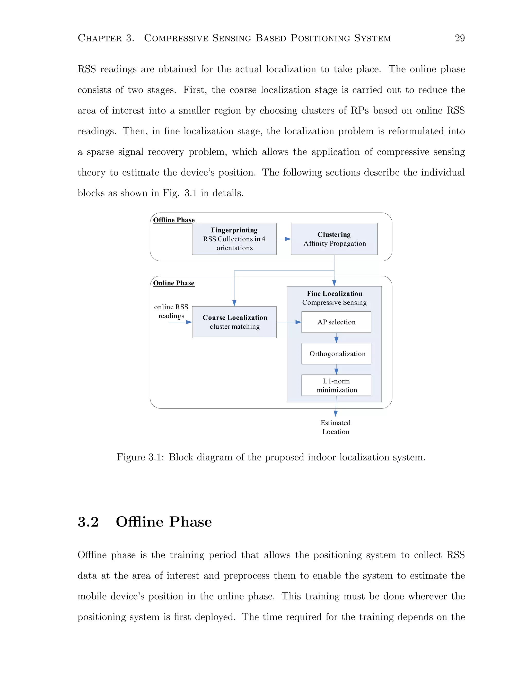
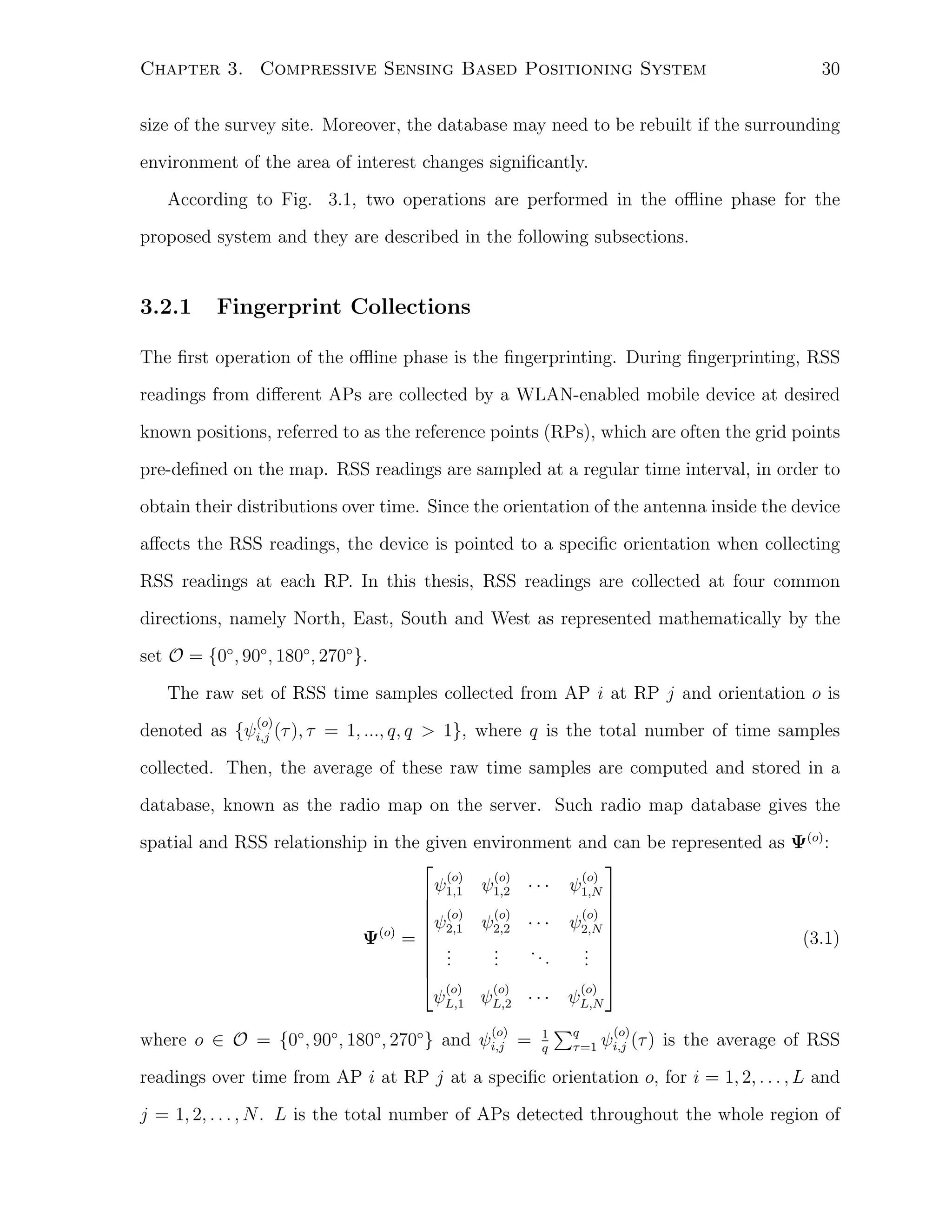
44. Chapter 3. Compressive Sensing Based Positioning System
31
interest and N is the total number of RPs. The columns of Ψ(o) represent the average
RSS readings at each RP, which can be referred to as the radio map vector and is denoted
as
(o)
(o)
ψ j = [ψ1,j
(o)
ψ2,j
···
(o)
ψL,j ]T ,
j = 1, 2, . . . , N
(3.2)
Besides the average RSS reading matrix Ψ(o) , the database server also stores the
variance of these time samples, which are useful in determining which APs should be
selected for localization. The variance vector for each RP is defined as
(o)
(o)
∆j = [∆1,j
(o)
where ∆i,j =
1
q−1
∑q
(o)
τ =1 (ψi,j (τ )
(o)
∆2,j
···
(o)
∆L,j ]T ,
j = 1, 2, . . . , N
(3.3)
(o)
− ψi,j )2 is the unbiased variance of RSS readings from
AP i at RP j for orientation o.
For each RP j, its position represented as Cartesian coordinates (xj , yj ), together with
its average and variance of the RSS readings from different APs at different orientations
(o)
(o)
form a set of (xj , yj ; ψ j ; ∆j ), o ∈ O, which is stored in the fingerprint database. The
database is then preprocessed as described in the next subsection before being used for
the computation of position estimation during online phase. Note that if there is no RSS
readings collected from an AP at a RP and an orientation, the corresponding value in
the fingerprint database is set to a small value to imply its invalidity.
3.2.2
Clusters Generation by Affinity Propagation
Due to the time varying characteristics of the indoor propagation channel, RSS readings
collected during online phase may deviate from those stored in the radio map database.
As a result, these deviation may lead to error estimation of position. In addition, the
computation time for finding position updates increases proportionally to the number of
RPs. Therefore, a coarse localization stage is introduced at the online phase to confine
the localization problem into a smaller region, namely a subset of RPs that have similar
RSS readings to the online measurement, before the fine localization is performed. This

45. Chapter 3. Compressive Sensing Based Positioning System
32
stage can effectively reduce the computation time due to the reduction of number of
relevant RPs, as well as the errors introduced by the potential outliers.
The RPs collected in the offline phase are required to be divided into subsets, so that
a coarse localization stage can take place during the online phase. The RPs whose RSS
readings are similar and physically close to each other should belong to the same group.
This group division process, which is referred to as the clustering process in the proposed
system is done during the offline phase after the fingerprints collection is finished. Since
the RSS readings for the same RP vary for the four orientations, the clustering process
is performed on each of the four radio map databases separately.
The affinity propagation algorithm described in Section 2.5 is used to generate the
desirable clusters, as this algorithm allows all the RPs to have equal chances to be
exemplars and is easily to be implemented. It requires two input parameters, namely the
similarity between pairs of RPs and the preference values. At orientation o, the similarity
between RP i and RP j is defined as
(o)
(o)
s(i, j)(o) = −∥ψ i − ψ j ∥2 , ∀i, j ̸= i ∈ {1, 2, ..., N }, o ∈ O
(3.4)
Since all of the RPs are equally desirable to be exemplars, their preferences are set
to a common value. In order to generate a moderate number of clusters, the common
preference for orientation o is defined as
p(o) = γ (o) · median{s(i, j)(o) , ∀i, j ̸= i ∈ {1, 2, ..., N }}, o ∈ O
(3.5)
where γ (o) is a real number which is experimentally determined, such that a desired
number of clusters is generated.
For each orientation, o ∈ O, the affinity propagation algorithm takes the above definitions of similarity (3.4) and preference (3.5) as inputs and then it recursively updates
the responsibility messages and availability messages according to (2.12) to (2.15) until
a good set of exemplars and the corresponding clusters emerges [15]. This set of generated exemplars is denoted as H(o) and the corresponding cluster member set with RP

46. Chapter 3. Compressive Sensing Based Positioning System
33
(o)
j as the exemplar is represented as Cj , j ∈ H(o) . In general, the RPs that are within
the same cluster should be physically in close proximity, as the neighboring RPs should
attain similar RSS readings. However, due to the varying characteristics of RSS readings
(such as the shadowing effects), there exist RPs that are physically far away from their
assigned clusters. These RPs, referred to as outliers, are manually assigned back to the
clusters that are physically closeby to reduce the potential errors in position estimations.
3.2.3
Interaction between the database server and the mobile
device during offline phase
Fig. 3.2 illustrates how the proposed positioning system is set up on the mobile device
and the server during offline phase to obtain and process the training data required for the
localization. The mobile device collects RSS time samples from detectable APs at specific
positions (RPs) and transmits these data to the server. After the fingerprint collection is
done by the device, the server creates the radio map database and generates clusters for
each orientation by applying the affinity propagation algorithm. This algorithm is run
on the server as it is an iterative process that consumes a large amount of memory and
processing power that may not be supported by the mobile device. At the end of the
offline phase, the server obtains the coordinates of the RPs, radio map matrices, variance
of RSS readings and also clusters information for each orientation. These data are then
used in the online phase for the computation of position estimations.
3.3
Online Phase
During the online phase, the device, carried by a mobile user and pointed to an unknown
orientation, collects online RSS readings from detectable APs, which are then used together with the fingerprint database to estimate the device’s location. The online RSS

47. Chapter 3. Compressive Sensing Based Positioning System
Mobile Device
34
Server
Collect RSS time samples from APs
at RP j for 4 orientations
Compute the average and variance of
RSS readings over time, _j (o), _ j(o)
∆
ψ
Send RP j’ s information:
_j (o), _j (o) & coordinates (x_j, y_j)
SEND
Collect fingerprint for RP j
in 4 orientations
∆
Use the device to
collect N RPs
ψ
Create overall radio map matrix:
(o)
= [ _ 1(o), _ 2(o),…, _N (o)]
ψ
ψ
ψ
Ψ
Apply affinity propagation on each
radio map to generate sets of
exemplars H(o) and their
corresponding members C_j (o)
Outlier adjustment
for each radio map
Figure 3.2: Interaction between the database server and the mobile device during offline
phase.
measurement vector at time t is denoted as
r(t) = [r1 (t), r2 (t), · · · , rL (t)]T
(3.6)
where {rk (t), k = 1, ..., L} is the online RSS readings from AP k at time t. Since the
positioning system does not take into account the previous estimate, the time dependency
notation (t) is dropped in this chapter for simplicity purpose, i.e. the online RSS reading
is denoted as r instead of r(t).
As shown in Fig. 3.1, the collected measurement vector is the input to the proposed
positioning system. First, it is used in the coarse localization stage to reduce the area of
interest. Then it is also used in the fine localization stage to obtain the final estimated
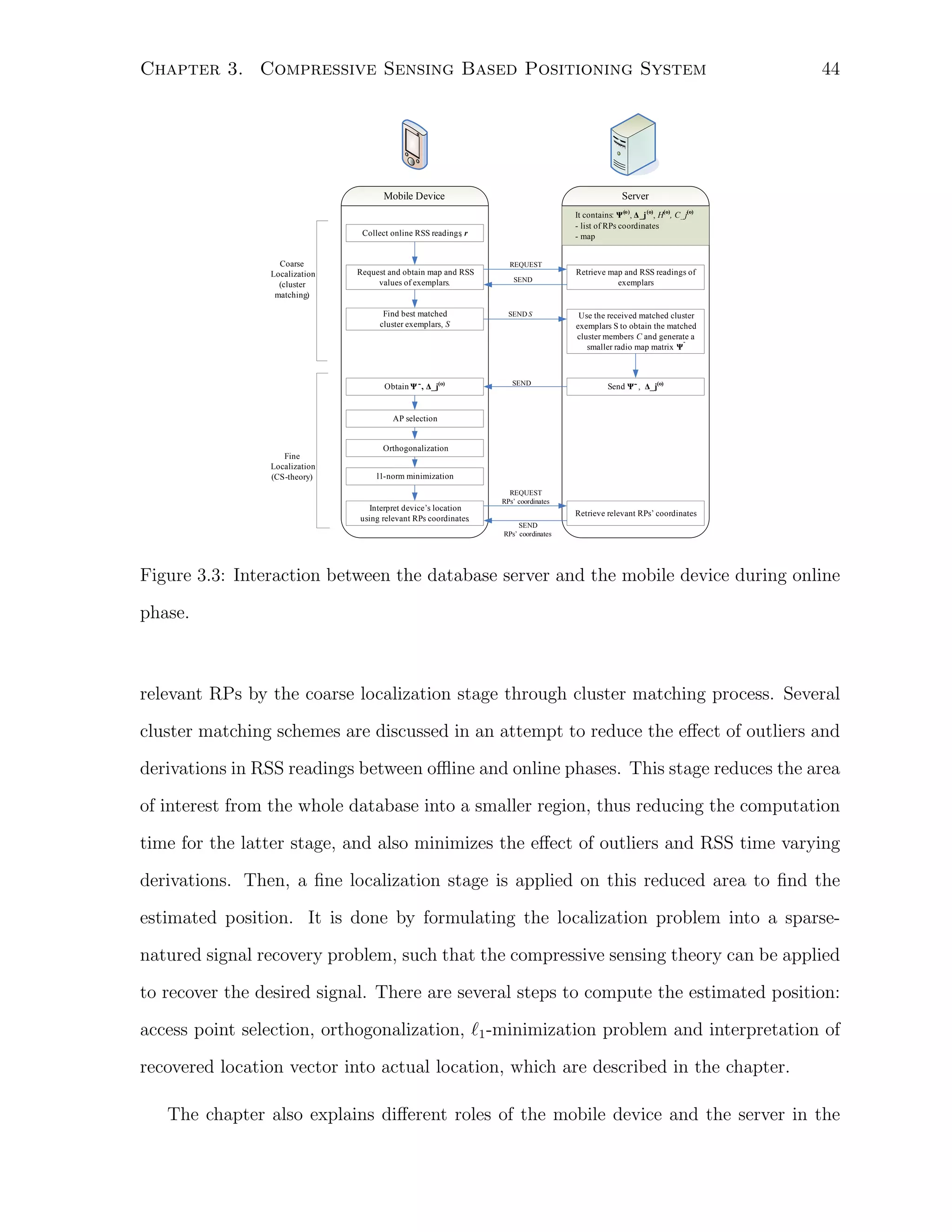
position. The details of these two stages are described in the following sections.

48. Chapter 3. Compressive Sensing Based Positioning System
3.3.1
35
Coarse Localization Stage: Cluster Matching
As mentioned earlier, the goal of the coarse localization stage is to reduce the region of
interest from the whole fingerprint database to a subset of it. Thus, it can reduce the
computation time for the fine localization stage, as fewer RPs are considered. It can also
confine the maximum localization error to be the size of this subset, whereas this error can
be much larger when no coarse localization stage is implemented. The coarse localization
is done by selecting the clusters, as defined in the offline phase, whose RSS radio map
vectors best-match with the online RSS measurement vector r. Since the target device
can be physically located at the boundaries of the defined clusters, a few best-matched
clusters, instead of only one cluster, are selected to eliminate the inaccuracy due to the
edge problem.
The cluster matching process can be interpreted as finding a set of best-matched
exemplars SRSS with their corresponding cluster members set CRSS , such that they have
the highest similarities with the online reading. It is crucial to have a good similarity
function between the online reading r and an exemplar j ∈ H(o) , ∀o ∈ O, denoted
as SM atch (r, j)(o) , so that the clusters for which the online measurement vector r should
belong to can be correctly identified. The worst case scenario, where wrong sets of clusters
are chosen for the online measurement vector r, should be avoided, as this results in a
wrong localization region and thus introduces large localization error. This may happen,
as the online RSS readings may deviate from the fingerprint database due to the time
varying indoor radio propagation channel. In order to reduce the occurrences of such
scenarios, several matching schemes are considered in this thesis. These schemes provide
different ways to define the appropriate similarity function SM atch (r, j)(o) .
1. Exemplar based cluster matching
This is the most basic scheme, which uses the same definition as (3.4) for the
clustering in offline phase. The similarity computes the Euclidean distance of the

49. Chapter 3. Compressive Sensing Based Positioning System
36
online measurement vector r to the individual exemplar’s RSS radio map vector
from each cluster:
(o)
SM atch (r, j)(o) = −∥r − ψ j ∥2 ,
∀j ∈ H(o) ,
∀o ∈ O
(3.7)
2. Average based cluster matching
Instead of using the exemplar RSS radio map vector, the average of the RSS radio
map vectors of all the cluster members, which gives a more comprehensive and
representative readings of the whole cluster, is used to compute the Euclidean
distance against the online measurement vector r:
SM atch (r, j)(o) = −∥r −
∑
1
(o)
|Cj |
(o)
k∈Cj
(o)
ψ k ∥2 ,
∀j ∈ H(o) , ∀o ∈ O
(3.8)
3. Weighted Average cluster matching
This scheme takes into account the stability of the RSS readings from a specific
AP at different RPs. Different weights are added to the similarity function for each
AP of each cluster at each orientation, so that it gives more weight to the stable
RSS readings. The stability of an AP at a RP can be determined as the inverse of
the variance of the RSS readings collected from that AP at that RP calculated in
the offline phase, thus APs with smaller variances are more reliable and have larger
weights. The similarity function is defined as:
(o)
SM atch (r, j)(o) = −∥Wj · (r −
(o)
Wj
1
∑
(o)
|Cj |
(o)
k∈Cj
(o)
ψ k )∥2 , ∀j ∈ H(o) , ∀o ∈ O
√

(o)
w1,j
0
···
0


√


(o)
 0
w2,j 0
0 


= .

..
 .

.
0
0 
 .


√
(o)
0
···
0
wL,j
(3.9)
(3.10)

50. Chapter 3. Compressive Sensing Based Positioning System
(o)
where Wj
37
(o)
is the diagonal weight matrix and wl,j , l = 1, 2, . . . , L is the weight of
AP l for cluster j at orientation o. This weight is proportional to the inverse of the
variance of the AP for the specific cluster, namely
(o)
wl,j ∝
1
¯ (o)
∆
l,j
¯ (o)
∆l,j =
1
(3.11)
∑
(o)
|Cj |
(o)
k∈Cj
Then these weights are normalized, so that
(o)
∆l,k
∑L
k=1
(3.12)
(o)
wl,j = 1.
4. Strongest APs matching
In this scheme, the online measurement vector is first pre-filtered to determine L′
APs that have the strongest RSS readings. Then, the similarity can be calculated
using any of the above schemes by only considering the RSS readings from these
selected APs. Since the APs that have stronger RSS readings tend to be more
stable as the device is with high probability within their coverage area, whereas the
APs with weaker signals tend to vary in time, the scheme is able to provide good
matching similarity definition by only considering the reliable APs.
All the above cluster matching schemes attempt to reduce the possibility of choosing
the wrong clusters used by the fine localization and thus improving the system’s stability
and accuracy. The performances of these schemes are evaluated in details in Chapter 7.
By evaluating the similarity function described above, the set of best matched exemplars SRSS with their corresponding cluster members set CRSS can be found as:
SRSS = {(j, o)| SM atch (r, j)(o) > α, j ∈ H(o) , o ∈ O}
(o)
CRSS = {(k, o)| k ∈ Cj , (j, o) ∈ SRSS }
(3.13)
(3.14)
where α is a predefined threshold value to determine whether a cluster should be included
into SRSS . Since only a few set of clusters are desired to be included in SRSS , α is set to

51. 38
Chapter 3. Compressive Sensing Based Positioning System
be a high percentage, α1 , of the maximum similarity difference, that is
α = α1 ·
max
j∈H(o) ,o∈O
{
}
SM atch (r, j)(o) + (1 − α1 ) ·
min
j∈H(o) ,o∈O
{
SM atch (r, j)(o)
}
(3.15)
Finally, the region of interest of the localization problem can be reduced to the set of
˜ ˜ ˜
CRSS . The modified radio map matrix ΨL×N , N = |CRSS | can be obtained as
(o)
˜
Ψ = [ψ j , ∀(k, o) ∈ CRSS ].
(3.16)
This matrix will then be used by the following fine localization stage. Note it is
possible that this matrix may contain the radio map vectors from the same RP but at
different orientations, as all clusters from different orientations are considered for cluster
matching.
3.3.2
Fine Localization Stage: Compressive Sensing Recovery
The fingerprint-based localization problem can be reformulated as a sparse signal recovery
problem, as the position of the mobile user is unique in the discrete spatial domain. By
assuming that the mobile user is located exactly at RP j and facing at orientation o, such
that (j, o) ∈ CRSS , the user’s location can be represented relative to these RPs instead
of the actual location. The mathematical representation is a 1-sparse vector, denoted as
θ N ×1 , whose elements are all equal to zero except the n-th element, so that θ(n) = 1,
˜
where n is the corresponding index of the RP at which the mobile user is located, that is
θ = [0, ..., 0,
1
, 0, ..., 0]T
(3.17)
nth element
Then, the online RSS measurement r obtained by the mobile device can be expressed
as:
˜
y = Φr = ΦΨθ + ε
(3.18)
˜
where Ψ is the modified radio map matrix as defined in (3.16) and ϵ is an unknown
measurement noise. The matrix ΦM ×L is an AP selection operator applied on the online

52. 39
Chapter 3. Compressive Sensing Based Positioning System
RSS measurement vector r to obtain vector y, where M < L is the desired number of
APs to be selected.
Based on this sparse signal recovery formulation, the following parts explain how the
location of the mobile user can be recovered by using the compressive sensing theory.
A. Access Points Selection
Since most modern buildings are equipped with a large number of APs to ensure good
quality of wireless services, the total number of detectable APs in these buildings, L is
often much greater than that required for positioning. These extra APs lead to excessive
computations and possibly biased estimations if some of the APs are not reliable. Inclusion of RSS readings from unstable APs may introduce error to the estimations, as online
RSS values may deviate from the readings in the offline database. Therefore, an access
point selection step is introduced to select a subset of reliable and stable APs from the
available ones to be used for the actual positioning, in order to eliminate the errors due
to large number of APs. Denote the set of all available APs found within all the RPs by
L with |L| = L. Then the AP selection step is to determine a subset of APs, M ⊆ L,
such that |M| = M ≤ L.
The AP selection process is carried out by applying the AP selection operator Φ on
the online measurement vector r as defined in (3.18). Each row of Φ, is a 1 × L vector
th
that selects the desired lm AP, where lm ∈ M, by assigning ϕ(lm ) = 1 and zero to the
rest of the elements, namely:
ϕm = [0, ..., 0,
1
, 0, ..., 0],
lm ∈ M, ∀m = 1, 2, . . . , M
(3.19)
lm −th element
In this thesis, three AP selection schemes are used based on APs stabilities and
differentiability in spatial domain. Their performances are evaluated in a later chapter.
1. Strongest APs [39]

53. Chapter 3. Compressive Sensing Based Positioning System
40
This scheme selects the set of M APs with the strongest RSS readings from the
online RSS measurement vector. These APs with strong RSS readings are more
reliable than the ones with weak RSS readings, as they provide a high probability
of coverage over time. The set of APs can be obtained by sorting the elements
of the online measurement vector r in descending order and selecting indices of
the first M values that correspond to the APs with highest RSS readings. Since
the online RSS readings are different for each run, the AP selection operator Φ is
created dynamically on the device for each update during the online phase.
2. Fisher Criterion [38, 66]
This scheme selects the APs which discriminate themselves the best within RPs.
The discrimination ability for each AP i, i ∈ {1, 2, . . . , L} can be quantified through
the Fisher criterion. The metric for AP i, denoted as ξi is defined as
∑
ξi =
(o)
(j,o)∈CRSS (ψi,j
∑
(j,o)∈CRSS
¯
where ψi =
1
˜
N
∑
(j,o)∈CRSS
¯
− ψi )2
(o)
(3.20)
∆i,j
(o)
ψi,j . The APs with highest ξi are chosen to construct
the AP selection operator Φ for the actual localization. This metric accounts
for two factors: the denominator ensures that RSS values should not vary too
much over time, thus implies that the offline and online values are similar and
the numerator evaluates the discrimination ability of each AP by considering the
strength of variations of mean RSS across RPs. Since this metric calculations are
done across the RPs j at orientation o chosen in the coarse localization stage,
(j, o) ∈ CRSS , the AP selection operator Φ is created dynamically on the device for
each update during the online phase.
3. Random Combination
Unlike the above two schemes, which select the appropriate APs based on different
criteria and create the AP selection operator Φ dynamically for each update, the

54. Chapter 3. Compressive Sensing Based Positioning System
41
random combination scheme does not take into account the performance of the
APs and thus have less computation complexity during online phase and also does
not require large number of RSS time samples for the variance calculation in the
offline phase as required by the Fisher criterion. The AP selection operator Φ is
defined as a randomly generated i.i.d. Gaussian M × L matrix. Thus, according to
(3.18), y = Φr, y is a set of M linear combinations of online RSS values from L
APs. Since the same matrix can be reused for each update, it can be generated and
stored first during the training period and retrieved for use directly in the online
phase, saving the time to dynamically generate the matrix as required by the other
two schemes.
B. Orthogonalization and Signal Recovery using ℓ1 -minimization
Compressive sensing theory requires both sparsity and incoherence of the signal, so that
it can be recovered accurately. Although the localization problem as defined in (3.18)
˜
satisfies the sparsity requirement, Φ and Ψ are in general coherent in the spatial domain.
Thus, an orthogonalization procedure is applied to induce the incoherence property as
required by the CS theory [67, 68].
The orthogonalization process is done by applying an orthogonalization operator, T,
on the vector y, such that z = Ty. The operator is defined as
T = QR†
(3.21)
˜
where R = ΦΨ, and Q = orth(RT )T , where R† is a pseudo-inverse of matrix R and
orth(R) is an orthogonal basis for the range of R. By applying this operator on y, (3.18)
becomes:
z = Ty = QR† y
= QR† Rθ + QR† ε
= Qθ + ε′
(3.22)

55. Chapter 3. Compressive Sensing Based Positioning System
42
˜
where ε′ = Tε. If M is in the order of log N , the minimum bound required by the
CS theory, θ can be well-recovered from z with very high probability, by solving the
following ℓ1 -minimization problem [67, 68].
ˆ
θ = arg min ∥θ∥1 ,
s.t. z = Qθ + ε′ .
(3.23)
˜
θ∈RN
The computation complexity of the ℓ1 -minimization algorithm grows proportional to
the dimension of vector θ, which is the number of potential RPs. Therefore, the coarse
localization stage, which reduces the area of interest from all the N RPs into a subset
˜
of N < N RPs, reduces the computational time and resources required for solving the
ℓ1 -minimization problem, and thus allows this procedure to be carried out by resourcelimited mobile devices.
C. Interpretation of Actual Position
The above procedure is able to recover the exact position, if the mobile user is located at
one of the RPs facing one of the orientations in the set of O, which is the assumption made
earlier in order to formulate the localization problem into a 1-sparse natured problem.
However, in real situation, the mobile user may not be located at an RP facing a certain
ˆ
orientation. Thus, in actual implementation, the recovered position vector θ is not a
1-sparse vector, rather a vector with a few non-zero coefficients. A post-processing step
ˆ
is conducted to interpret this recovered location vector θ into an actual location and
compensate the error induced by the grid assumption. The procedure chooses the set of
ˆ
all indices of the dominant elements in θ, which are above a certain threshold λ, denoted
as R
ˆ
R = {n|θ(n) > λ}
(3.24)
ˆ
λ = λ1 max(θ)
(3.25)
where λ1 is a parameter within a range (0, 1) and is adjusted experimentally. Then, the
estimated location of the mobile user can be calculated as a weighted average of these

56. Chapter 3. Compressive Sensing Based Positioning System
43
ˆ
potential candidate points, using the normalized value in θ as the corresponding weight
for each potential RP, that is
p = (ˆ, y ) =
ˆ
x ˆ
∑
ηn · (xn , yn )
(3.26)
n∈R
∑
ˆ
ˆ
where ηn = θ(n)/ n∈R θ(i) and (xn , yn ) is the cartesian coordinates of RP n.
3.3.3
Interaction between the database server and the mobile
device during online phase
The roles of the mobile device and the server during the online phase are illustrated in
Fig. 3.2. First, the device collects the online RSS readings from all the detectable APs,
namely r. Then the device requests the map and the representative RSS readings for each
cluster from the server, in order to perform coarse localization. After the best-matched
clusters are found, the device communicates with the server to obtain the relevant radio
˜
map matrix Ψ for the following fine localization. The device carries out steps of AP
selection, orthogonalization and ℓ1 -minimization to obtain the recovered location vector
ˆ
θ. Finally, the device asks the server for the potential candidate RP’s coordinates and
ˆ
computes the estimated position according to θ.
3.4
Chapter Summary
In this chapter, the proposed compressive sensing based positioning system is described
in details. The system involves two phases. The offline phase is the training period
that collects RSS values from detectable access points at reference points to create the
fingerprint database. It also runs the affinity propagation algorithm to create different
clusters of RPs with similar RSS reading patterns and within physical proximity. The
actual localization takes place in the online phase, which consists of two stages. First,
the mobile device collects the online RSS readings, which are used to find the subset of

57. Chapter 3. Compressive Sensing Based Positioning System
Mobile Device
Coarse
Localization
(cluster
matching)
Server
Collect online RSS readings r
,
44
It contains: Ψ (o), ∆_j (o), H(o), C_j(o)
- list of RPs coordinates
- map
REQUEST
Request and obtain map and RSS
values of exemplars.
SEND
Retrieve map and RSS readings of
exemplars
Find best matched
cluster exemplars, S
SEND S
Use the received matched cluster
exemplars S to obtain the matched
cluster members C and generate a
smaller radio map matrix Ψ
Obtain Ψ ͂ , ∆_j(o)
SEND
Send Ψ ͂ , ∆_j(o)
͂
AP selection
Orthogonalization
Fine
Localization
(CS-theory)
l1-norm minimization
Interpret device’s location
using relevant RPs coordinates.
REQUEST
RPs’ coordinates
Retrieve relevant RPs’ coordinates
SEND
RPs’ coordinates
Figure 3.3: Interaction between the database server and the mobile device during online
phase.
relevant RPs by the coarse localization stage through cluster matching process. Several
cluster matching schemes are discussed in an attempt to reduce the effect of outliers and
derivations in RSS readings between offline and online phases. This stage reduces the area
of interest from the whole database into a smaller region, thus reducing the computation
time for the latter stage, and also minimizes the effect of outliers and RSS time varying
derivations. Then, a fine localization stage is applied on this reduced area to find the
estimated position. It is done by formulating the localization problem into a sparsenatured signal recovery problem, such that the compressive sensing theory can be applied
to recover the desired signal. There are several steps to compute the estimated position:
access point selection, orthogonalization, ℓ1 -minimization problem and interpretation of
recovered location vector into actual location, which are described in the chapter.
The chapter also explains different roles of the mobile device and the server in the

58. Chapter 3. Compressive Sensing Based Positioning System
45
proposed system. The server is mainly served as a database storage, which when requested by the device, sends required information, such as map and RSS readings to
the device. It is also responsible for running the affinity propagation algorithm to form
clusters during offline phase, as the device does not have enough computation resources
to run such clustering scheme. The mobile device collects the RSS readings and obtains
information from the server, in order to estimate its location locally.

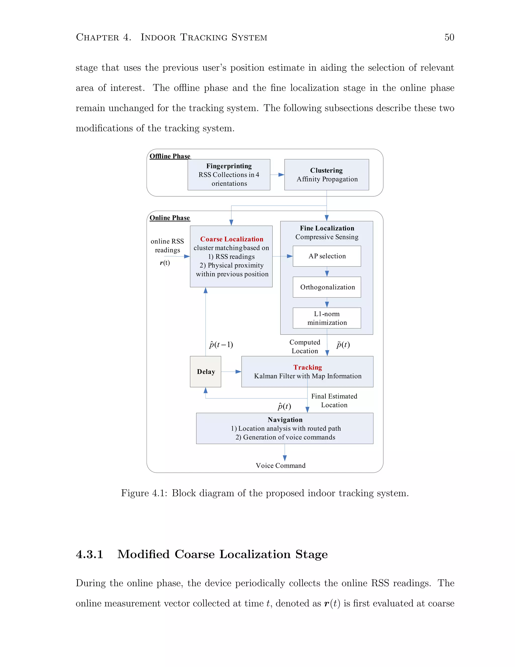
59. Chapter 4
Indoor Tracking System
The previous chapter describes a positioning system that can accurately estimate a stationary user’s position. This positioning system is modified in this chapter in order to
track the dynamic mobile user. The proposed indoor tracking system uses the Kalman
filter with map information to smooth out the location estimate and also uses previous
position estimate to choose the relevant region of interest in the coarse localization stage.
This chapter first describes the Kalman filter and then the proposed indoor tracking
system.
In this chapter, the tracking problem is defined as follows. The device carried by
the mobile user periodically collects the online RSS readings from each APs at a time
interval ∆t, which is limited by the device’s network card and hardware performances.
The online RSS readings vector is denoted as r(t) = [r1 (t), r2 (t), . . . , rL (t)], t = 0, 1, 2, ...,
where rl (t) corresponds to the RSS from AP l at time t. Then, the indoor tracking system
uses these RSS readings to estimate the user’s location at time t, which is denoted as
p(t) = [ˆ(t), y (t)]T .
ˆ
x
ˆ
46

60. Chapter 4. Indoor Tracking System
4.1
47
General Bayesian Tracking Model
The tracking problem of a mobile user can be modeled by a general Bayesian tracking
model as follows [41] and [47]:
x(t) = ft (x(t − 1), w(t))
(4.1)
z(t) = ht (x(t), v(t))
(4.2)
where x(t) = [x(t), y(t), vx (t), vy (t)] is the state of the user at time t with (x(t), y(t))
as the Cartesian coordinates of the user’s location and vx (t) and vy (t) as the velocities
in x and y directions, respectively. Assuming the tracking is a Markov process of order
one, the state evolves as a function ft of previous state and w(t), i.i.d. process noise
vector only. In addition, the measurement z(t) depends on the current state and the
i.i.d. measurement noise vector v(t) through the function ht .
The current location of the mobile user, x(t) can then be estimated recursively from
the set of measurements up to time t, i.e. z(1 : t) = {z(i), i = 1, ..., t}, in terms of the
probability distributive function (pdf), denoted as p(x(t)|z(1 : t)). Assuming that the
initial pdf p(x0 |z 0 ) ≡ p(z 0 ) and p(x(t−1)|z(1 : t−1)) are known, the pdf p(x(t)|z(1 : t))
can be obtained by the following prediction and update stages:
1. Prediction Stage:
The prior pdf p(x(t)|z(1 : t−1)) can be predicted based on p((x(t)|x(t−1)), which
is defined by the state process equation (4.1) and the previous state pdf.
∫
p(x(t)|z(1 : t − 1)) =
p((x(t)|x(t − 1))p(x(t − 1)|z(1 : t − 1))dx(t − 1) (4.3)
2. Update Stage:
Then, the prior pdf can be updated by the measurement z(t) obtained at time t

61. 48
Chapter 4. Indoor Tracking System
using the Bayes’ rule,
p(z(t)|x(t))p(x(t)|z(1 : t − 1))
p(z(t)|z(1 : t − 1))
∫
p(z(t)|z(1 : t − 1)) = p(x(t)|z(1 : t − 1))dx(t)
p(x(t)|z(1 : t)) =
(4.4)
(4.5)
where p(z(t)|x(t)) is defined by the measurement model (4.2).
4.2
Kalman Filter
If the process and measurement noises are assumed to be Gaussian and the motion
dynamic model is linear, i.e. the process and measurement functions ft and ht are linear
in equations (4.1) and (4.2), then the general Bayesian tracking model is reduced to
a Kalman filter. The optimal solution can be obtained for this Kalman filter as the
minimum mean square estimates (MMSE). The process and measurement equations of
the Kalman tracking model can be formulated as
x(t) = Fx(t − 1) + w(t)
(4.6)
z(t) = Hx(t) + v(t)
(4.7)
where x(t) = [x(t), y(t), vx (t), vy (t)]T is the state vector and z(t) is the measurement
vector. The process noise w(t) ∼ N (0, S) and the measurement noise v(t) ∼ N (0, U)
are assumed to be independent with the corresponding covariance matrices S and U.
The matrices F and H in (4.6) define the linear motion model. For the tracking
problem, they are assigned as follows:


1 0 ∆t 0




0 1 0 ∆t


F=



0
0 0 1


0 0 0
1


1 0 0 0
H=

0 1 0 0
(4.8)
That means the current location of the mobile user is assumed to be the previous location
of the user plus distance traveled, which is computed as the time interval ∆t times the

62. 49
Chapter 4. Indoor Tracking System
current velocity, and is corrupted with Gaussian noise. The current measurement should
be the current location subject to Gaussian noise.
By assigning the initial conditions of x(0) and P(0), the steps to obtain the final
ˆ
estimates of state vector x(t) and the error covariance P(t) are computed as follows:
ˆ
1. Prediction Stage
x− (t) = Fˆ(t − 1)
ˆ
x
(4.9)
P− (t) = FP(t − 1)FT + S
(4.10)
K(t) = P− (t)HT (HP− (t)HT + U)−1
(4.11)
x(t) = x− (t) + K(t)(z(t) − Hˆ− (t))
ˆ
ˆ
x
(4.12)
P(t) = (I − K(t)H)P− (t)
(4.13)
2. Update Stage
For each time step t, the measurement vector z(t) in (4.12) is the current user’s estimated location computed by the positioning system. After the state vector is estimated,
the final filtered estimate of the user’s location can be found as:
p(t) = Hˆ(t)
ˆ
x
4.3
(4.14)
Overview of Proposed Indoor Tracking System
The Kalman filter can be applied on the CS-based positioning system described in the
previous chapter to improve the accuracy in estimating the dynamic user’s trajectory.
Fig. 4.1 shows the proposed indoor tracking system that is built on top of the CS-based
positioning system. As compared to Fig. 3.1, there are two major modifications for the
tracking system. Besides the introduction of the Kalman filter stage after the end of
the fine localization stage, the tracking system also has a different coarse localization

63. 50
Chapter 4. Indoor Tracking System
stage that uses the previous user’s position estimate in aiding the selection of relevant
area of interest. The offline phase and the fine localization stage in the online phase
remain unchanged for the tracking system. The following subsections describe these two
modifications of the tracking system.
Offline Phase
Fingerprinting
RSS Collections in 4
orientations
Clustering
Affinity Propagation
Online Phase
online RSS
readings
r(t)
Fine Localization
Compressive Sensing
Coarse Localization
cluster matching based on
1) RSS readings
2) Physical proximity
within previous position
AP selection
Orthogonalization
L1-norm
minimization
ˆ
p (t − 1)
Delay
Computed
Location
p (t )
Tracking
Kalman Filter with Map Information
ˆ
p (t )
Final Estimated
Location
Navigation
1) Location analysis with routed path
2) Generation of voice commands
Voice Command
Figure 4.1: Block diagram of the proposed indoor tracking system.
4.3.1
Modified Coarse Localization Stage
During the online phase, the device periodically collects the online RSS readings. The
online measurement vector collected at time t, denoted as r(t) is first evaluated at coarse

64. 51
Chapter 4. Indoor Tracking System
localization stage to reduce the area of interest by selecting the relevant RPs in the
database for the fine localization stage. In addition to using the online RSS readings to
find the relevant RPs, the tracking system also uses the previous user’s position estimate
to select the appropriate RPs. Fig. 4.2 depicts the coarse localization stage employed
by the tracking system. The modified coarse localization stage chooses the relevant RPs
based on two criteria: Group I) online RSS readings, and Group II) physical proximity
of previous estimate.
Fingerprint
Database
r(t)
Group I
Choose clusters of RPs
with similar RSS
CRSS
Find Common
RPs
ˆ
p (t − 1)
Group II
Choose RPs within
physical proximity
C
CDist
O
Figure 4.2: Coarse localization stage for the proposed tracking system.
Group I: RPs with similar online RSS readings
The system first selects the clusters of RPs defined in the offline stage that have similar
RSS reading patterns to the online RSS vector r(t). This cluster matching process is the
same as that described in Section 3.3.1. In summary, the system uses one of the cluster
matching schemes to evaluate the cluster matching similarities to the online RSS vector,
i.e. {SM atch (r(t), j)(o) , ∀j ∈ H(o) , ∀o ∈ O} and then selects the best-matched clusters
CRSS according to (3.13).

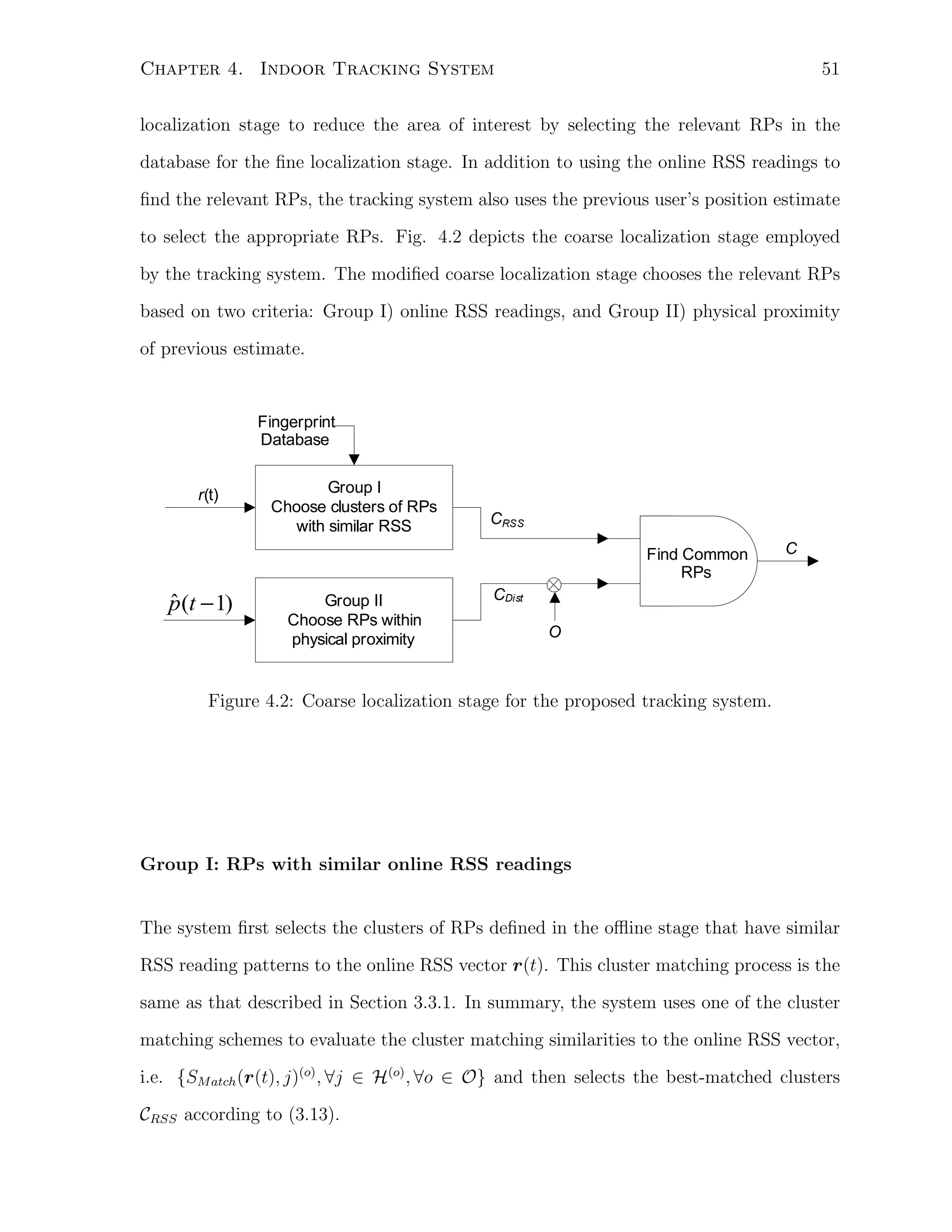
65. Chapter 4. Indoor Tracking System
52
Group II: RPs within physical proximity
Besides the use of the online RSS readings to choose the relevant RPs, they can be
chosen by finding the possible range of the device’s current location based on the previous
estimated location, p(t − 1) = (ˆ(t − 1), y (t − 1)). Since a person cannot walk far away
ˆ
x
ˆ
within a short period of time, it is reasonable that the system can limit the region of
interest into the possible walking range based on the previous estimated position, if it is
known and reliable. There are two schemes to choose this possible walking range and are
discussed as follows.
1. Unpredicted - Based only on previous estimation
This scheme selects a set of RPs that are within walking distance during the specified update time interval to the previous estimated location, that is
√
ˆ
ˆ
CDist = {j| (xj − x(t − 1))2 + (yj − y (t − 1))2 < β, j ∈ {1, . . . , N }}
(4.15)
where (xj , yj ) is the location of RP j and β is the walking distance within the
specified update time interval ∆t.
2. Predicted - Based on previous estimation and prediction using linear motion model
This scheme uses the previous estimated location to predict the current possible
location based on a linear motion model and then chooses the RPs which are within
the walking range of this predicted position. The same linear model used by the
Kalman filter defined in (4.8) and (4.6) without the addition of Gaussian noise can
¯
be used to predict the user’s current locations, denoted as p(t):
p(t) = HF¯(t − 1)
¯
x
(4.16)
where x(t − 1) = [ˆ(t − 1), y (t − 1), vx (t − 1), vy (t − 1)]T is the state vector with
¯
x
ˆ
ˆ
(ˆ(t − 1), y (t − 1)) = p(t − 1) as the previous user’s estimated position computed by
x
ˆ
the tracking system. The velocities in x and y directions, represented as vx (t − 1)

66. 53
Chapter 4. Indoor Tracking System
and vy (t − 1), respectively, can be defined in several ways. First, if both of them
are set to zeros, then the predicted location is the same as the previous estimate,
ˆ
p(t) = p(t − 1). This is equivalent to the previous described scheme. Second, if
¯
the user is known to be walking at a constant speed, these values can be assigned
accordingly. However, for real applications, a user may walk to a random direction
at a random speed. Thus, it is necessary to find a way to predict the user’s velocity
at each time interval, in order to have a good estimation for the current location.
The estimation of these velocities can be obtained from the output of the Kalman
filter, which is implemented after the fine localization stage and will be described
in Section 4.3.2. Then, the state vector for (4.16) can be assigned directly as the
final estimate of the state vector for the Kalman filter, i.e. x(t − 1) = x(t − 1).
¯
ˆ
The system then selects a set of RPs which are in close proximity to this predicted
current location p(t) = [¯1 (t), p2 (t)]T , that is:
¯
p
¯
CDist
√
¯
¯
= {j| (xj − p1 (t))2 + (yj − p2 (t))2 < β, j ∈ 1, . . . , N }
(4.17)
After the selection of these two groups of relevant RPs based on RSS readings similarities and physical proximities, the system then includes the common RPs that appear
in both groups as the set of reduced region, where the final localization stage is applied.
The common RPs is obtained as a set C,
C = CRSS
∪
{(j, o)|j ∈ CDist and o ∈ O}
(4.18)
This set contains RPs that satisfy both conditions of similar RSS readings to the
online RSS measurement and within close range to the user’s previous location. Thus,
they are very likely to be the possible locations that the current user is located. By
introducing the constraint of physical range, the system is able to identify the instants
when the online RSS readings collected is not useful to find the user’s position. In normal
operation, the user must be within a range around his previous location. If the selected

67. 54
Chapter 4. Indoor Tracking System
clusters of RPs in CRSS are far away from the previous location, then the online RSS
readings can be regarded as invalid, as there are large deviations between the online
readings and offline database, so that the cluster matching based on similarities of RSS
readings fails to find the correct clusters of RPs. This scenario leads to an empty set of C
and halts the fine localization stage. If such thing occurs, the system discards this online
RSS measurement vector and obtains a new one to restart the localization process.
There may be a possibility that all the consecutive online RSS measurement vectors
lead to empty sets of C. This makes the system continuously collect a new online RSS
measurement, which is then discarded, preventing it from computing the true estimate of
the user’s location. This happens as the previous position estimate is not accurate and
hence the selection of RPs based on such estimate does not match with the RPs selected
based on the online RSS measurement vector. Thus, the system is reset to use only the
online RSS measurement vector to select the RPs, when Nempty consecutive online RSS
measurement vectors are discarded, arguing that the previous position estimate is no
longer valid to reduce the localization problem into a smaller relevant region.
After a successful computation of finding the non-empty set of C, the modified radio
˜ ˜ ˜
map matrix ΨL×N , N = |C| can be obtained as
(o)
˜
Ψ = [ψ j , ∀(j, o) ∈ C].
(4.19)
This matrix will then be used by the fine localization stage. The fine localization
stage for the tracking system remains the same as the one in the CS-based positioning
system, which is already described in Section 3.3.2. Since the estimated user’s position
computed by the fine localization stage is then fed into the Kalman filter to obtain the
˜
final estimate in the tracking system, such temporal solution is referred to as p(t) in this
chapter, which indicates that it is not the final solution.

68. 55
Chapter 4. Indoor Tracking System
4.3.2
Map-Adaptive Kalman Filter
˜
After the computation of the location estimate, p(t) at the end of the fine localization
stage, the Kalman filter described in Section 4.2 is applied to enhance the tracking
˜
performance. By substituting z(t) = p(t) into the Kalman filter updating equations
ˆ
(4.9) to (4.14), the final estimated position p(t) can be obtained from the estimated
ˆ
state x(t) according to (4.14).
In real situation, the Kalman filter is able to enhance the tracking performance when
the user is walking along a corridor inside a building, as the linear motion assumed by
the filter is sufficient to model the user’s trajectory. However, when the user is making a
turn at an intersection, the linear model does not apply on this behavior which involves
abrupt change in direction and hence the Kalman filter requires several more updates to
reflect the user’s true trajectory and thus leads to more errors in position estimate.
This issue can be addressed by updating the Kalman filter according to the map
information. Since the Kalman filter behaves the best when the user is walking straight
along a corridor but performs poorly around the intersections, the Kalman filter is reset
when the user is in the region of intersection. Prior to the actual tracking, the map of
region of interest is studied to extract a list of intersections which are represented as noni
i
rotated bounding boxes, denoted as a set Rintersection = {(xi , ymin ), (xi , ymax )| i =
min
max
i
i
1, ..., B}, where (xi , ymin ) and (xi , ymax ) are the lower-left and upper-right corners
min
max
respectively of intersection i and B is the number of intersections found on the map.
Thus, the user is within the intersection region i at time tturn if the below two conditions
are satisfied:
ˆ
xi ≤ x(tturn ) ≤ xi
max
min
i
ymin
≤ y (tturn ) ≤
ˆ
(4.20)
i
ymax
When the user is within any of the intersection regions, the Kalman filter is reset
by reassigning the state vector and covariance matrix at time tturn , which are the initial

69. 56
Chapter 4. Indoor Tracking System
conditions for this new Kalman filter. Namely,
x(tturn ) = [p(tturn ), 0, 0]T
ˆ
ˆ
(4.21)
P(tturn ) = P(0)
Then, the Kalman filter is updated as normal according to (4.9) to (4.13) for the next
estimate at time (tturn + 1) using z(tturn + 1) = p(tturn + 1). This removes the inaccurate
˜
estimation by the Kalman filter when the user is making a turn. Fig. 4.3 summarizes
how the Kalman filter is applied on the proposed tracking system.
4.4
Chapter Summary
This chapter modifies the CS-based positioning system described in the previous chapter
into a tracking system, which is able to improve the accuracy in estimating the mobile
user’s locations. By using the user’s previous estimated locations, the tracking system
is able to refine the current estimate in two ways: 1) to select appropriate RPs in the
coarse localization stage and 2) to apply Kalman filter for better location estimate.
First, during the coarse localization stage, a set of RPs that are within walking range
to the i) previous estimated location p(t − 1) or ii) the predicted current location p(t)
ˆ
¯
based on the previous estimated location, are selected as the potential region of interest,
arguing that a user cannot be physically far away within a short period of time in the
indoor environment. The RPs appeared in both set of CDist , found based on previous
estimated location and the set of CRSS , determined by the original cluster matching
scheme for the CS-based positioning system, are then used to generate a modified radio
˜
map matrix Ψ that is required for the fine localization stage. This modified coarse
localization stage ensures that the reduced region of interest are within the walking
range of the user and provides a way to reject the invalid online RSS readings when no
common RPs are found in both sets.
The tracking system also introduces the Kalman filter stage, which uses the temporal

70. Chapter 4. Indoor Tracking System
Given:
i
i
Intersections Set: Rintersection = {(xi , ymin ), (xi , ymax )| i = 1, ..., B}
min
max
Inputs:
Computed estimate from fine localization stage: p(t)
˜
Final estimate of previous update: p(t − 1) = (ˆ(t − 1), y (t − 1))
ˆ
x
ˆ
Outputs:
Final estimate of current update: p(t) = (ˆ(t), y (t))
ˆ
x
ˆ
Kalman Filter:
Initial conditions
x(0) = [p(0), 0, 0]T , P(0)
ˆ
ˆ
Check if user is already at intersection
for i = 1, . . . B
i
i
if (xi ≤ x(t − 1) ≤ xi
ˆ
ˆ
min
max and ymin ≤ y (t − 1) ≤ ymax ) then
At intersection, reset Kalman filter
x(t − 1) = [p(t − 1), 0, 0]T
ˆ
ˆ
P(t − 1) = P(0)
break for loop
endif
endif
Update
set z(t) = p(t) to update the Kalman filter through (4.9) to (4.13)
˜
compute for p(t) according to (4.14)
ˆ
Figure 4.3: Map-Adoptive Kalman Filter
57

71. Chapter 4. Indoor Tracking System
58
position estimation, p(t), computed at the end of the fine localization stage as the input
˜
to update the previous estimated location p(t − 1) into the current final estimation p(t).
ˆ
ˆ
Since the Kalman filter performs poorly when the user makes turns and thus does not
follow the linear model, the proposed tracking system is designed to reset the Kalman
filter whenever the user is in an region of intersection, which is a possible place for the
user to make turns.

72. Chapter 5
Simple Navigation System
The proposed indoor tracking system can be implemented on mobile devices to provide
reliable and accurate real-time location estimates of the mobile user and thus is adequate
to provide location based services to the user. As an illustration and a way to evaluate
the performance of the tracking system, a simple navigation system is designed and
implemented on top of the tracking system to provide real-time guidance to the user to
reach the desired destination. The design and the implementation of such navigation
system is described in details in this chapter.
5.1
Overview of Navigation System
The goal of the navigation system is to decide a path between the user’s current location
and his desired destination and then provide guidance, which can be in the form of voice
instructions to let the user follow this planned path. In addition, the location updates,
{p(t), t = 1, ...}, generated periodically by the tracking system are fed into the navigation
ˆ
system to generate adequate instructions that are helpful to the user to get familiar with
the surrounding area. All of these operations require a detail map database that stores all
the map-related data for path routing and guidance. Fig. 5.1 illustrates the navigation
system. It consists of a map database, which is generated at the initial set up to provide
59

73. 60
Chapter 5. Simple Navigation System
the required map information for the navigation system; a path routing module, which
generates the path that leads the user to reach the destination and a tracking update
analysis module, which generates appropriate voice instructions according to the user’s
locations.
Initial Setup
Map Database Generation
- represent the layout as a connected graph
- define coordinates of special map features
- create audio files for all possible voice commands
During Real-Time
Navigation
Indoor Tracking System
User-defined
destination
ˆ
p (t )
ˆ
p(0)
Path Routing Module
ˆ
p (t )
Routed path
Yes
Tracking Update
Analysis Module
Require
reroute?
No
Voice Instructions
Figure 5.1: Navigation System Overview
5.2
Map Database Generation at Initial Setup
The navigation system relies heavily on the map of the region of interest, which illustrates
the layout of different features such as rooms, corridors, elevators, etc. For the initial
setup, different map features are extracted from the map, which allow the system to
generate a feasible path and descriptive instructions about the surrounding to the user
during the actual navigation process. The map database generation can be divided into
two operations: i) to represent the map layout as a connected path and ii) to define
locations of the map features.

74. Chapter 5. Simple Navigation System
5.2.1
61
Layout Definition
The layout of the map is interpreted as a connected graph, so that the path routing
problem can be transformed into a graph problem [56], which is solved by the path
routing module described in the later section. The nodes of this graph are a set of
Cartesian coordinates of the possible passage points along the corridors or destinations.
Two nodes are connected together with an edge, if both nodes can reach each other
physically without obstacles in their ways. A non-negative weight is assigned to each
edge and is defined as the Euclidean distance between the connected nodes. In order to
ensure that at least one feasible path can be generated for all the destinations defined on
the map, the graph must be connected meaning that there must be a path, which is a
set of edges that connect any pairs of nodes defined in this graph. This connected graph
can be represented as G = (E, V ), where E is a set of edges and V is a set of nodes. The
weight of the edges can be represented as a matrix DG = [dGij ]|V |×|V | , where dGij th entry
corresponds to the Euclidean distance between node i and node j if they are connected
by an edge, otherwise the value is set to infinity which implies the two nodes are not
connected to each other.
5.2.2
Map Features Definition
In order to provide more information about the surrounding environment, which will be
useful to help user to get familiar with the area, a list of map features can be extracted
from the map to generate a more comprehensive map database for the navigation system. This list of the map features can include general facilities and accesses and can be
expanded as needed depending on user’s preferences. Washrooms, elevators and stairs
are some examples of map features that are of interest to users. The list of the features
j
can be stored as a set Fmap = {(pj , Featurej ), j = 1, ..., nF }, where pj = (xj , yf ) is the
f
f
f
location of feature j and Featurej is the feature’s name and nF is the total number of

75. Chapter 5. Simple Navigation System
62
map features defined on the map.
5.3
Path Routing Module
At the beginning of the actual navigation, the device first obtains the user’s input of
the desired destination and user’s current location, which can be either specified by the
user or estimated by the device using the proposed tracking system. Then, the system
identifies the source node, vsource and the target node, vtarget on the connected graph
predefined in the setup stage, that are closest to the user’s current location and the
destination, respectively. The path routing problem is interpreted as finding the shortest
path between these two nodes on the connected graph [56]. This problem can be easily
solved by applying the Dijkstra algorithm, which is described in [69] and is summarized
in Fig. 5.2.
5.3.1
Path Analysis
After a set of nodes sequence, P, which constitutes the shortest path from the user’s
current position to the destination, is generated, the path is then analyzed to produce
necessary navigation information to the user.
The generated path is first divided into series of line segments, such that consecutive
line segments are pointing at different directions and the connected point between the
two segments becomes the turning point. This set of line segments extracted for the path
P can be denoted as Pl = {ℓ1 , ℓ2 , ...ℓS }, where S is the total number of line segments
i
i
and each segment is denoted as ℓi = {pi , pi }, where pi = (xi , ys ) and pi = (xi , ye )
e
e
s
s
e
s
are the starting and ending points of the ith line segment, respectively. The turning
points are identified as the ending points between line segments, that is T = {pi |i =
e
1, . . . , S − 1}. Based on these generated line segments, the system is able to determine
the turning points, the direction of turns and the distance traveled at each line segment

76. 63
Chapter 5. Simple Navigation System
Given:
Connected graph of the map layout with weight: G(E, V ), DG = [dGij ]|V |×|V |
Inputs:
User’s current location: p(t) → Source node: vsource
ˆ
Destination location → Target node: vtarget
Outputs:
A list of nodes of the shortest path from target node to source node: P
Dijkstra:
Initializations:
d = [d(1), ..., d(|V |)];
{d(vi ) = ∞, ∀vi ̸= vsource ∈ V },
e = [e(1), ..., e(|V |)];
{e(vi ) = −1, ∀vi ∈ V }
d(vSource ) = 0
Vunvisited := V
Actual operations:
while Vunvisited is not empty
u = arg min d,
remove u from Vunvisited
Vunvisisted
exit while loop if d(u) = ∞ or u == vtarget
for each v in Vunvisited
exit foreach loop ifdGuv == ∞
a = d(u) + dGuv ;
if a < d(v) then
d(v) = a;
Determine path sequence:
u := vtarget ,
P = {}
insert u at beginning of P and u := e(u) while e(u) ̸= −1
Figure 5.2: Dijkstra Algorithm
e(v) = u

77. 64
Chapter 5. Simple Navigation System
which facilitate the analysis of the user’s current locations in the tracking update analysis
module.
In addition, the system also finds out a list of relevant map features that appeared
along this generated path. For each line segment i, the system chooses the map features
from the set Fmap that are within βf meters from the line segment i and form a set
i
i
Fpath ⊆ Fmap . These sets {Fpath , i = 1, . . . , S} are useful for the system to effectively
determine if the user is close to these map features when he is following the path correctly,
and thus save the system from searching the full map feature set Fmap for each tracking
update.
5.4
Tracking Update Analysis Module
Tracking Module
(periodic update )
ˆ
p (t )
Reach destination ?
(1)
(2)
(3)
(4)
(1)
(5)
(6)
(7)
No
Match to one of line No
segments in path?
Yes
Voice Generation Engine
(7)
Yes
Routing
Module
For Noffpath
consecutive
updates
“Please wait for rerouting”
“Go straight”
“Prepare to turn left /right”
“Turn left/right”
“Wrong direction”
“<map feature> is on your left/right”
“You have arrived at <destination>”
(5)
(3), (4)
Is walking in wrong
direction ?
No
(2)
Yes
For Nwrong direction
consecutive updates
(6)
Determine if user
turn left or right
Yes
Yes
Near end of the line
segment?
No
Are there any
nearby map
feature?
No
Figure 5.3: Tracking update analysis
After the generation of the path that can lead the user to his targets, the device

78. 65
Chapter 5. Simple Navigation System
starts the tracking system to keep track of user’s position. For each tracking update,
the analysis module compares the location estimate to the routed path to check if the
user follows the path properly and then generate voice instructions when necessary. The
analysis process is illustrated in Fig. 5.3.
5.4.1
Analysis Process
The analysis module first determines if the user already reaches the destination by checking the Euclidean distance between the user’s current position and the target being within
a range of βdestination . If the user is at the destination, the module generates the voice instruction stating that the destination is reached and stops tracking system and navigation
module automatically.
ˆ
ˆ
ˆ
p(t ) = ( x(t ), y(t ))
p ie = (xie, yie )
p
i
i
i
i
p s = (x s, y s )
Figure 5.4: A point in close range to a line segment
Otherwise, the module attempts to match the user’s current position p(t) to one of
ˆ
the line segments in the generated path set Pl . If this tracking update is close to line
segment ℓi as illustrated in Fig. 5.4, then we can find the projection and the minimum
distance of the tracking update point p(t) to the line segment ℓi by solving the two
ˆ
equations [70]:
pi = pi + µi (pi − pi )
s
e
s
(5.1)
(p(t) − pi ) · (pi − pi ) = 0
ˆ
s
e
(5.2)
where pi is the projected point which is collinear with pi and pi , and µ is the ratio in
e
s
terms of the distance between pi and pi indicating how far the point pi is away from pi .
s
e
s

79. Chapter 5. Simple Navigation System
66
By substituting (5.1) into (5.2), the solution to µi is
µi =
(p(t) − pi ) · (pi − pi )
ˆ
s
e
s
∥pi − pi ∥2
s
e
(5.3)
If the computed µi is within the range [0, 1], then the projected point falls onto the line
segment, which implies that the update estimate is within the range of this line segment.
By substituting (5.3) back into (5.1), the projected point pi can be computed and the
shortest distance of the tracking update point to the line segment can be obtained as
di = ∥p(t) − pi ∥.
ˆ
min
The system determines that the tracking estimate p(t) follows the line segment ℓi if
ˆ
i) µi ∈ [0, 1] and ii) di < βpath . If there are consecutively Noffpath tracking estimates
min
failing to match with any of the line segments in Pl , the analysis module assumes that
the user does not follow the path properly. Thus, the analysis module will ask the user
to stop walking and inputs the user’s current position as the starting point to the path
routing module to reroute an alternate path for the user to reach the destination.
The value of µi is also a good indicator to tell if the user is walking along the path
properly. In normal situation, where the user follows the path correctly, the value of µi
should increase from zero to one along the same line segment ℓi for consecutive tracking
updates and then eventually move to the next segment ℓi+1 , where the value of µi is no
longer valid and the value of µi+1 is then computed. Thus, when µi , i < S is close to
one, this indicates that the user is close to the end of the line segment ℓi , where a turn is
required for the user to move to the next line segment ℓi+1 . The direction of turn can be
determined by finding the positive angle difference, ∆ρi between the two vectors that are
formed by joining the starting and ending points of the current and next line segments
as illustrated in Fig. 5.5. For simplicity, the module only identifies either a left or right
turn.
The module assumes a very simple scheme to determine the orientation of the mobile
user. For each tracking update, a direction vector is computed between the current update
and the previous one and then is compared with the currently matched line segment

80. 67
Chapter 5. Simple Navigation System
1) ∆ρ i = ρ i +1 − ρ i
2) if ∆ρ i < 0°, then ∆ρ i = ∆ρ i + 360°
pie = (x ie, yie ) = Pi+1s = (x i+1s, yi+1s )
ρ i +1
3) if ∆ρ i ≈ 90°, then it is a right turn
ρi
else if ∆ρ i ≈ 180°, then it is a left turn
pis = (x is, yis )
P
i+1
i+1
e
= (x
e,
y
i+1
e
)
Figure 5.5: Determining the direction of turn based on the two line segments ℓi and ℓi+1
direction. If consecutive Nwrong
direction
tracking updates are in opposite direction of the
line segment, then a voice command of wrong direction is issued to the user.
Finally, the analysis module computes the Euclidean distance between the user’s
i
current estimate p(t) to the map features in Fpath , where i corresponds to the line segment
ˆ
i that the user is currently following. If the distance is smaller than βf , then the module
will generate the corresponding voice command regarding this specific map features to
the user.
5.4.2
Voice Generation
The voice instructions of the analysis module can be generated on-the-fly by using textto-speech (TTS) engine. However, TTS engines are not readily available for free to be
used on smart devices and render delays in giving real-time instructions to the user. Thus,
the navigation system uses an alternate method to obtain the voice commands. Since the
navigation system only has a small library of instructions, all of these commands are first
created and saved as audio files during initial setup. The audio can be generated from
R
text by using the online AT&T Natural Voices⃝ Text-to-Speech Demo [71]. Then, the
analysis module determines which instructions are needed and plays the corresponding
audio files. Although these audio files occupy extra amount of memory spaces on the
smart devices, the system is able to generate reliable voice instructions in real time, which

81. Chapter 5. Simple Navigation System
68
may not be achievable by using the TTS engines.
5.5
Chapter Summary
This chapter describes the navigation system that is built on top of the tracking system
to provide guidance to the user. The navigation system requires an initial setup to
extract information from the map and generates pre-determined voice instructions that
are used by the actual navigation process. The navigation system is then divided into two
modules. One is the path routing module, which takes in the user’s current location and
desired destination as inputs to generate a feasible path based on the connected path
defined according to the layout of the map and identifies the turning points and map
features found along this path. Then, the tracking update analysis module uses the path
information along with the current user’s estimated position to determine the appropriate
voice instructions to be given to the users. This navigation system is implemented on
the smartphone and its details are found in the next chapter.

82. Chapter 6
Software Implementation on Mobile
Devices
This chapter describes how the indoor CS-based positioning and tracking system, along
with the navigation application described in Chapters 3 to 5 are implemented as a software on the PDAs and smartphones.
6.1
Software Platform
The software is developed on PDAs and smartphone that are installed with Windows Mobile operating systems to implement the proposed indoor tracking and navigation system.
Unlike Android platform [72], which has become popular just recently and only available on android-powered smartphones, the Windows Mobile platform has been developed
maturely and in addition to Window Mobile-powered smartphones, such platforms have
also been used on PDAs. The development of software application for the iPhone is also
ruled out as the wifi scanning functionality, which is the core requirement for the indoor
tracking system, is not provided by the Apple’s official software development kit (SDK).
Although there are private libraries available online to provide that function, they require
the jailbreaking of the iphone and thus violate the Apple’s development license [73], [74].
69

83. 70
Chapter 6. Software Implementation on Mobile Devices
The software is written in C# using Microsoft .Net Compact Framework version 3.5 in
Visual Studio 2008. It utilizes two open source libraries available on the internet to relieve
the burden on developing the application on this platform. They are the OpenNetCF
library [75] and the DotNetMatrix library [76], which provide the WiFi RSS scanning
functions and basic matrix operations respectively.
6.2
Devices in Testing
The developed software has been deployed onto three different devices and their specifications in comparison to a standard laptop of the same price level (around $ 600) are
shown in Table 6.1 [77–80].
Devices
Processor
RAM
Speed
Window Mobile
WLAN
Version
hx4700
PDA2: HP iPAQ 624 MHz
128 MB
hx2750
Smartphone:
800 MHz
256 MB
Pocket PC 2003 802.11b
1
ple/second
Pocket PC 2003 802.11b
1
2nd
64 MB
ning Rate
2nd
PDA1: HP iPAQ 624 MHz
ple/second
Professional
802.11b/g 0.67
Samsung Omnia II
Dell
Inspiron
WiFi Scan-
sam-
sam-
sam-
ple/second
15 2.2 GHz
4 GB
Windows 7
802.11g
Laptop
Table 6.1: Devices Specifications
It is obvious that the PDAs and smartphone have much more restricted resources in
processing power and memory than a standard laptop. Thus, indoor tracking systems
that use probabilistic approach [38] and particle filters [47, 51, 81] that require large
computation power may not be realizable on these devices. The proposed indoor tracking

84. Chapter 6. Software Implementation on Mobile Devices
71
system is implemented on these devices to illustrate that such system is a compact
algorithm that is able to provide real-time and accurate estimate of user’s location. The
performances of these devices are evaluated in Chapter 7.
Note that the Samsung smartphone is equipped with an accelerometer and a digital
compass. By using the Samsung Mobile SDK [82], the software is able to access these two
sensors. The maximum sampling interval that can be set by the SDK for these sensors
is 200 milliseconds. Attempts have been made to let the system utilize both sensors in
aiding to determine the user’s travel distances and orientations. However, the phone is
incompetent to handle both sampling of the sensors’ data and scanning the WiFi RSS
from APs at the same time and thus the program becomes unstable and often crashes
unexpectedly. Besides, the sampling rate and the response are too slow for both sensors
to let the system obtain useful real-time data within a short time interval for the tracking
updates. Thus, these sensors are not incorporated into the proposed tracking system in
this thesis.
Both of the PDAs use the WiFi network adaptor as the basic wireless connection
method, unlike the smartphone, which cellular reception precedes the WiFi reception.
Thus, the signal strength level and the refresh rate of the WiFi antenna of the smartphone are inferior to the ones in PDAs. By using the OpenNetCF library, the software
is able to detect the WiFi adaptor on the devices and then scan the detectable APs
with their unique media access control (MAC) address as their identifications and their
RSS readings. All the three devices require a duration of one second to accomplish this
operation. However, tests have shown that the smartphone is required to wait for 500
milliseconds between each scanning operations, rather than 100 milliseconds for both
PDAs, in order to detect valid RSS readings, thus proved that the refresh rate for smartphone is slower. Since the PDAs have a faster refresh rate, the performance evaluations
in the next chapter are focused on these PDAs.

85. 72
Chapter 6. Software Implementation on Mobile Devices
6.3
Software Design
Samsung Mobile
SDK
IndoorLocalizerProg
OpenNetCF
OpenNetCF.Net
LocalizerBasicLibrary
IndoorLocResources
DotNetMatrixCF
MathAlgorithm
Localization
•
•
Tracking
•
•
Config.txt
Fingerprint Database with
clustered information
Map Database
Log files
Navigation
Figure 6.1: The overview of the software design. Arrows shows the dependency of the
libraries and blue colored boxes are the developed modules for the software.
The overall design of the software is illustrated in Fig. 6.1. The screenshot of the
PDA shows the menu of the software, which has five major operations. The flowchart on
the left of the screenshot shows the dependencies of the libraries of the software design
structure. The resources, such as the fingerprint and map databases, which are needed
by the software are stored in a folder on the PDA and represented as the cylindrical
shape on this figure.
6.3.1
Software’s Functionalities
As depicted in Fig. 6.1, the software has five major operations. They are:
1. Detect APs, which run the WiFi scanning function provided by the OpenNetCF
library and displays the MAC address and RSS for each detectable APs in table
format as depicted in Fig. 6.2

86. Chapter 6. Software Implementation on Mobile Devices
73
Figure 6.2: An example screenshot of Detect AP operation.
2. Collect Fingerprints, which let the user to properly setup the tracking system by
collecting fingerprints and defining the map features on the screen;
3. Localize Yourself, which runs the CS-based position system described in Chapter
3 and displays the user’s position on the screen;
4. Tracking, which periodically collects RSS readings and runs the tracking system
described in Chapter 4 and displays the user’s position on the screen;
5. Navigation, which asks the user’s input of destination and implements the navigation system described in Chapter 5.
6.3.2
Resources Folder
There is a folder on the device that contains all the required resources to run the tracking
and navigation system properly and is accessible by the software. This folder, IndoorLocResources, also contains a configuration setting file, namely Config.txt, which defines
the device in test, the map scale ratios and also all the parameters that can be adjusted
for the tracking and navigation system. In addition, an image file, which displays the

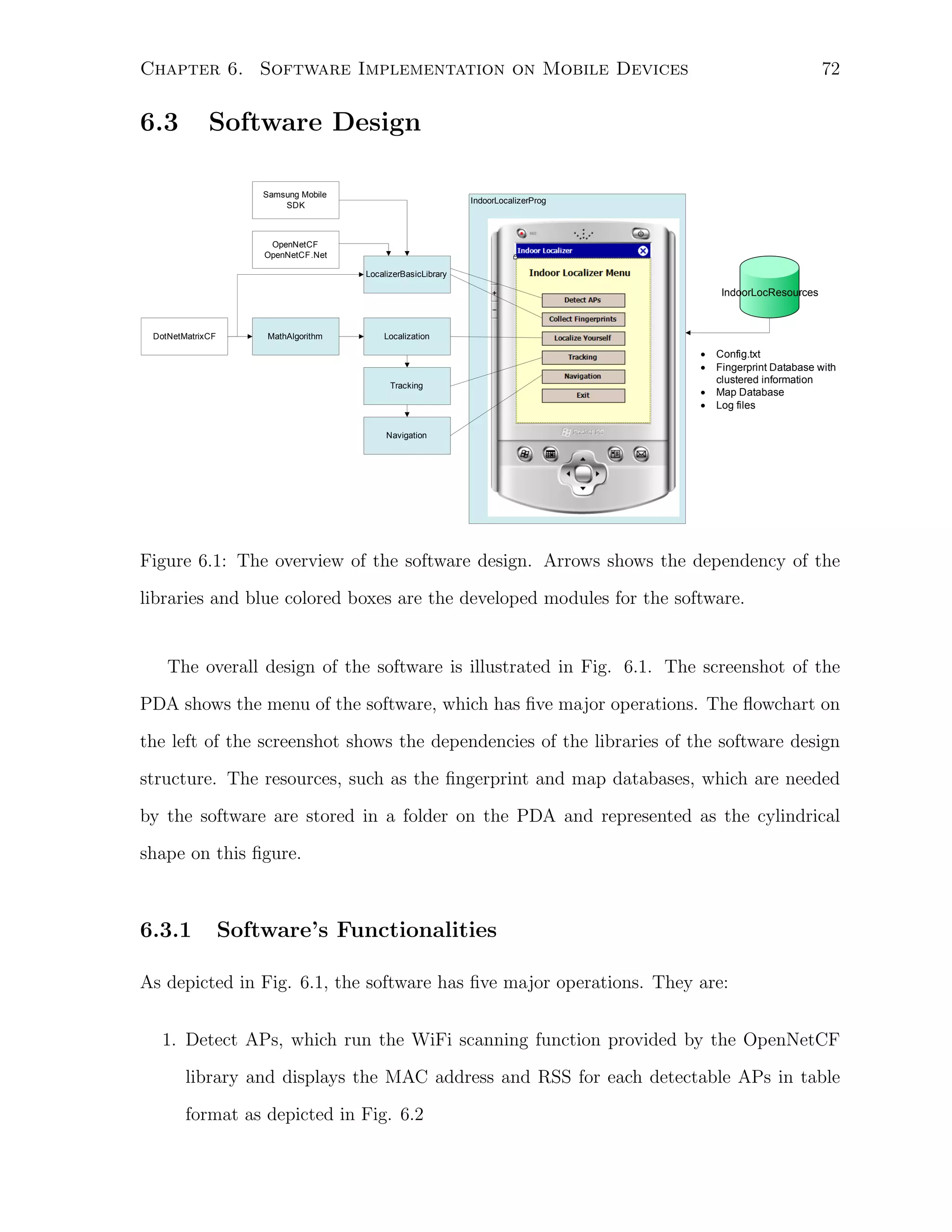
87. Chapter 6. Software Implementation on Mobile Devices
74
map of the region of interest, is included to allow the software to use it to collect fingerprints and displays user’s location properly on the screen. This image map is stored
as a bitmap format and is scaled, so that it can be showed properly on the screen of
smart devices. The same image map file is used by all the three devices and their image
pixel to actual distance meter scale is included in the Config.txt to allow the system to
estimate the actual distance according to the map. During the initial setup, the user
uses the Collect Fingerprint functions to collect fingerprint database and map features
which are all stored in this folder. The raw fingerprint database is then transferred to a
computer to generate clusters based on Section 3.2.2 using affinity propagation algorithm
and put this cluster information back to the PDA’s resources folder. Then, the online
operations: localization, tracking and navigation obtain the fingerprint database and the
map database from this folder to achieve their purposes.
6.3.3
Libraries’ Definitions
Fig. 6.1 shows that the software is divided into six blocks of libraries. These libraries
are organized so that each individual block deals with one specific task and allows the
developer to modify these codes easily. These libraries are:
• MathAlgorithm This library contains the math algorithms that are required by
the proposed system. It uses the open source library DotNetMatrix to perform
the standard matrix operations. The four algorithms defined in this library are i)
affinity propagation algorithm, which is converted from matlab code found in [15];
ii) ℓ1 -minimization by using primal-dual interior point method, known as basis
pursit, which is also converted from matlab code found in CS-solver ℓ1 -Magic [65];
iii) Dijkstra algorithm as depicted in Fig. 5.2 and iv) the Kalman Filter as defined
in Section 4.2. Although the affinity propagation algorithm is implemented, the
software can only handle the computation for a small number of collected RPs.
It complains for the lack of memory and crashes when the number of collected

88. Chapter 6. Software Implementation on Mobile Devices
75
fingerprints exceeds 15. Thus, the clustering process is done by a computer instead.
• LocalizerBasicLibrary This library provides the basic functions that are used by
the rest of the program. It uses the open source libraries OpenNetCF to obtain
the WiFi scanning function and the Samsung Mobile SDK to control the sensors
of the Samsung smartphone. In addition, the config file is read by this library to
set up the software to run properly with user’s defined parameters. The behavior
of the software during its launch is recorded in log files produced by this library
for later observation. Moreover, it contains the functions to collect and write the
fingerprint and map database into the IndoorLocResources folder.
• Localization This library implements the CS-based positioning system described
in Chapter 3. It refers to MathAlgorithm to solve the ℓ1 -minimization problem.
• Tracking This library implements the CS-based tracking system described in
Chapter 4. It is built based on the Localization and MathAlgorithm libraries.
• Navigation This library implements the navigation system described in Chapter
5. It refers to the MathAlgorithm library to run the Dijkstra algorithm for the
path routing module. In addition, it also includes functions to load and play the
voice instructions audio properly.
• IndoorLocalizerProg This is the main program of the software which defines the
user interface and connects all the libraries together to the desirable functionalities.
6.4
Chapter Summary
This chapter describes the software developed on the PDAs and smartphones for the
proposed indoor tracking and navigation system. The software is developed in C# using
Microsoft .Net Compact Framework version 3.5 for Windows Mobile-powered smartdevices. Besides the online operations that localize, track or navigate the user, the software

89. Chapter 6. Software Implementation on Mobile Devices
76
also includes the functions to collect offline fingerprint and map databases. In this thesis,
the software is deployed on three devices: two HP PDAs and one Samsung smartphone
to evaluate the performance of the proposed tracking and navigation system.

90. Chapter 7
Experimental Results
In this chapter, the proposed CS-based positioning and tracking system is evaluated in
different experimental sites using the devices mentioned in the previous chapter. Due to
the dynamic and unpredictable nature of the radio channel in indoor environment, the
RSS varies over time and cannot be modeled accurately by a propagation model. Thus,
RSS readings are collected in real indoor environments to evaluate the performance of
the proposed system. The results obtained by using different parameters for proposed
systems are also examined to illustrate the effect of these parameters. In addition, the
proposed systems are also compared with other positioning and tracking algorithms.
Finally, the implementation of the navigation system for the actual sites is also included.
7.1
7.1.1
Experimental Setup
Experimental Sites
The experiments took place at two different sites: i) Bahen Centre for Information Technology of the University of Toronto and ii) Canadian National Institute for the Blind
(CNIB). Their general information is summarized in Table 7.1.
The proposed positioning and tracking system can be directly used in the buildings
77

91. 78
Chapter 7. Experimental Results
Sites in Study
Dimensions
# of additional Total # Device
#
deployed APs
of APs
in Test
of
RPs
Bahen 4th Floor
30 m × 31 m 8
26
PDA1
72
CNIB 2nd Floor
35 m × 71 m 15
23
PDA2
128
Table 7.1: Comparison of experimental sites
that are already equipped with access points (APs), whose settings and positions are
unknown. Besides the original access points, several additional access points are deployed
in the experimental sites to ensure that the sites have enough reliable RSS readings to
estimate the locations accurately. The additional deployed APs denoted in Table 7.1 are
the off-the-shelf access points, Cisco Linksys Wireless-G Router WRT54G2, which are
set to have maximum transmission power 18dBm and set to transmit signals at channel
1. Note that all RSS readings collected by the devices are in dBm scale.
Bahen Center: Positioning Analysis
The first experimental site is a part of the fourth floor of the eight storey building, Bahen
centre at the University of Toronto [83]. The main focus of this site is to analyze the
performance of the CS-based positioning system as described in Chapter 3. The region
of interest is a office area with a L-shaped corridor with a dimension of 30 m × 31 m,
which is comparable to those experimented in [19, 28, 38, 49]. Including the 8 additional
deployed access points, which are spread across the whole area, a total of 26 access points
can be detected. Both the PDA1 and Smartphone as defined in Table 6.1 are used
for the fingerprint collection, but the analysis of the positioning system is mainly based
on the PDA1 device, as it can obtain a better RSS fingerprint database due to better
antenna and faster WiFi scanning rate than the Smartphone.

92. Chapter 7. Experimental Results
79
Fingerprint Collections For this experimental site, the PDA1 and Smartphone,
each carried by an individual, are used to collect the fingerprints during the offline phase.
At each RP, 50 RSS time samples from 26 APs were collected for each of the four orientations: North, East, South and West, by PDA1 and Smartphone with the sampling
rates of 1 sample/second and 0.67 sample/second respectively. If the devices cannot detect the RSS from a particular AP, a small default value of -110dBm is assigned to that
particular reading. A total of 72 RPs, which were evenly distributed along the corridors
of the site with an average grid spacing of 1.5m were collected on both devices over a
period of 5 days and 8 days for PDA1 and Smartphone respectively. These raw sets
of RSS readings are then processed to generate the required fingerprint database for the
positioning systems. Note that, the samples of default readings (-110dBm) are excluded
when calculating the average and variance of the RSS readings. The positioning system
is then evaluated by the following two RSS sets as the online RSS measurement vectors.
Validation Data The positioning system is first tested by a validation set, which is
extracted from the raw RSS readings of the fingerprint database. That is, at each of the
RPs, choose one of the 50 RSS time samples at one of the four orientations collected
by the device as the online RSS measurement vector to estimate the desired location,
which should be the location of the corresponding RP. This set is used to evaluate the
performance of the system under zero noise interference situation.
Stationary User Testing Data Another set of online RSS readings were collected
by the PDA1 on a different day to evaluate the performance of the system under timevarying environment. In order to obtain the actual locations of the user, the device let
the stationary user orientated at an arbitrary orientation to click on the map, which was
shown on the device’s touchscreen, where he was standing and then the device started the
WiFi scanning process. Each online observation was an average of 2 RSS time samples
which was taken over a period of 2 seconds. In total, 3 online observations of 48 locations

93. Chapter 7. Experimental Results
80
spread across the area of interest were collected as the stationary user set.
CNIB: Tracking and Navigation Analysis
The evaluation of the performance of the proposed tracking and navigation systems
described in Chapter 4 and 5 took place on the second floor of CNIB, located in midtown Toronto. Subject testings were also conducted at this site to evaluate the usefulness
of the navigation system to the visually impaired people. This building is designed to
provide easy accessibility to anyone, especially the visually impaired people [84]. The area
of dimensions 35 m × 71 m, which is larger than the experimental site at Bahen Centre,
consists of a main straight central hallway connected to a C-shaped small corridor that
leads to different conference rooms. Unlike the campus areas, such as the Bahen centre,
which are densely populated with access points, there are only a few APs detectable in
the CNIB. Thus, 15 additional APs are deployed throughout the whole area, creating a
total of 23 APs that can be used in the experiments. All the three devices described in
Table 6.1 are used to collect the fingerprint database, but the analysis of the tracking and
navigation systems is mainly focused on the PDA2 device, as it has the best fingerprint
database in terms of the number of real RSS readings from detectable APs, whereas the
other two devices often cannot obtain the RSS readings from APs during the sampling
periods.
Fingerprint Collections Similar to the fingerprint collection process at the Bahen
Centre, 50 RSS time samples were collected for each orientation at each RP by all the
devices, except the Smartphone, which only 40 RSS time samples were collected instead.
A total of 128 RPs, which were evenly distributed along the hallway and corridors with an
average grid spacing of 1.5m were collected by PDA2. The number of RPs collected by
the PDA1 (120 RPs) and Smartphone (126 RPs) varied slightly as they were operated
by different individuals. It took about 10 days to finish this offline phase.

94. 81
Chapter 7. Experimental Results
Mobile User Testing Data In order to evaluate the performance of the tracking
system, several traces were collected on a different day by PDA2. The user carried the
PDA2 device, which obtained RSS samples at every second, and walked at a constant
speed along 4 different traces, as summarized in Table 7.2. The actual locations of the
user for each step can be deduced based on the user’s speed and elapsed time.
Trace #
# of turns # Repetitions Distance Average Duration
1
2
4
53.63m
156.3s
2
2
4
29.43m
89.2s
3
0
4
30.80m
84.6s
4
4
2
91.84m
279.5s
Table 7.2: Traces Summary
7.1.2
Performance Benchmarks
The performance of the proposed positioning system is compared to two methods. The
first one is the KNN method [19], described in Section 2.2.1, which is a simple technique
that can be easily implemented on the mobile devices. In the following experiments, three
neighbors (k = 3) are used to estimate the user’s location. Another one is the kernelbased method [38], which is summarized in Fig. 2.1. The computation of this probabilistic
approach technique involves all the RSS time samples collected during the offline phase
and thus requires more processing time and resources. It may not be realizable by the
mobile devices, as they have limited processing power and memory.
As for the proposed tracking system, two performance benchmarks are used for comparison. They are the original proposed positioning system and the direct application of
the Kalman filter on the original proposed positioning system.

95. 82
Chapter 7. Experimental Results
7.1.3
Figure of Merit
The performance of the positioning and tracking systems can be evaluated in terms of
the position error, which is defined as the Euclidean distance between the actual location
and its estimation. The average root mean square error (ARMSE) is used as a metric
for the performance evaluations and it is defined below:
Average Root Mean Square Error (ARMSE)
The ARMSE for the stationary user is defined as:
Np
1 ∑
Np i=1
ARMSE
Ti
1 ∑
∥p − pi (t)∥2
ˆ
Ti t=1 i
(7.1)
where pi is the actual location for test point i and pi (t) is the estimated location for test
ˆ
point i using test sample t. Np and Ti are the number of test points and number of test
samples for test point i respectively.
Similarly, the ARMSE for the mobile user is defined as:
ARMSE
1
Ntrace
∑
Ntrace
i=1
Ni
1 ∑
∥p (t) − pi (t)∥2
ˆ
Ni t=1 i
(7.2)
where pi (t) and pi (t) are the actual and estimated locations for a particular trace i at
ˆ
step t. Ntrace is the number of traces and Ni is the number of steps of trace i.
7.2
Positioning Results on Bahen Fourth Floor
This section focuses on the evaluation of the implementation of proposed CS-based positioning system using the PDA1 device on the fourth floor of Bahen Centre.
7.2.1
RSS Distributions
RSS readings in an indoor environment vary due to several factors. The radio channel
impediments such as shadowing and multi-path propagation due to walls and obstacles,

96. Chapter 7. Experimental Results
83
the orientation of the antennas of the wireless devices, the movements of human bodies
are some of the causes that induce the time varying characteristics of the RSS, which
cannot be easily predicted by a radio propagation model. In this section, the RSS distributions collected by PDA1 and Smartphone on the Bahen fourth floor are examined
to illustrate these variations of RSS in indoor environment.
RSS Distribution Over Time
Fig. 7.1 depicts the histograms of RSS time samples from the same access points collected
by both devices at the same reference point. Both histograms show that the RSS varies
around the average values with certain variances. In this example, the mean and variance
of the RSS collected by PDA1 are -48dBm and 23dBm, whereas for Smartphone
(excluding the invalid -110dBm instances) are -68dBm and 18dBm respectively. The
RSS readings collected by Smartphone are much lower than the ones collected by
PDA1. This illustrates that the antenna gain for Smartphone is smaller than the one
for PDA1. In addition, there are several instances that Smartphone is not able to
detect any RSS (which is then assigned to a default value of -110dBm). This may be due
to the hardware limitation of the antenna of the Smartphone. The low quality antenna
of Smartphone makes it not as reliable as the PDA1 to be a WiFi-scanning device.
The actual RSS readings across time are shown in Fig. 7.2a. This figure further
illustrates that the RSS collected by PDA1 is much more stable and higher than the one
collected by Smartphone, thus the RSS data collected by the PDA1 is used for the
analysis of the CS-based positioning system applied on the Bahen fourth floor. Since the
average RSS values are used by the proposed positioning and tracking system to estimate
the user’s location, it is important to obtain a reliable average value. Fig. 7.2b depicts
the average RSS values against the number of RSS samples used. The average RSS for
PDA1 converges to -48dBm after 30 samples are used, thus the fingerprint database
that is generated from 50 time samples should be enough for the system.

97. 84
Chapter 7. Experimental Results
6
5
5
4
4
Frequency
7
6
Frequency
7
3
3
2
2
1
1
0
−55
−50
−45
−40
RSS Readings [dBm]
−35
−30
0
−120
(a) RSS collected by PDA1
−110
−100
−90
−80
RSS Readings [dBm]
−70
−60
−50
(b) RSS collected by Smartphone
Figure 7.1: Example histograms of RSS distributions of the same access point over 50
time samples for different devices pointing North at the same reference point on Bahen
fourth floor.
−45
−30
PDA1 − North
Smartphone − North
−40
−50
PDA1 − North
Smartphone − North
−50
RSS Average [dBm]
RSS readings [dBm]
−55
−60
−70
−80
−60
−65
−70
−90
−75
−100
−110
0
5
10
15
20
25
Time [s]
30
35
40
45
(a) RSS measurements over time
50
−80
0
5
10
15
20
25
30
Number of RSS time samples
35
40
45
50
(b) RSS averages across time samples
Figure 7.2: An example of RSS measurements over time and their averages with respect
to the number of time samples of the same access point for different devices at the same
reference point on Bahen fourth floor.
RSS Distribution Across Reference Points
The RSS distributions in spatial domain are shown in Fig. 7.3. Several observations are
made from these figures. First, the orientation of the antenna of the same device affects
the RSS variations slightly as illustrated in Fig. 7.3a. Second, the variations of RSS are
much larger when different devices are used as shown in Fig. 7.3b. However, the trends

98. 85
Chapter 7. Experimental Results
of the RSS distributions across the spatial domain are similar for all these cases. This
particular access point is located close to the 20th RP, thus the RSS at this RP is the
strongest and decreases as the RPs are moving away from the access point. Note that
there is a second peak of the RSS value at the 6th RP, as this RP is in the same corridor
where the AP is located.
−20
−20
PDA1 − North
PDA1 − South
PDA1 − North
Smartphone − North
−40
RSS Readings [dBm]
−30
−40
RSS Readings [dBm]
−30
−50
−50
−60
−60
−70
−70
−80
0
10
20
30
40
50
Reference Points Indices
60
(a) Different Orientations
70
80
−80
0
10
20
30
40
50
Reference Points Indices
60
70
80
(b) Different Devices
Figure 7.3: An example of averaged RSS of the same access point in spatial domain for
different orientations and different devices on Bahen fourth floor.
7.2.2
Offline Phase: Clustering Results by Affinity Propagation
The fingerprint database collected by the PDA1 are used for the analysis of the CS-based
positioning system. As described in Chapter 3, the fingerprints are first pre-processed
during the offline phase to generate clusters that are required for the later coarse location
stage.
Effect of Preferences on the Number of Clusters Generated
According to (3.5), γ (o) is determined experimentally to obtain desirable number of clusters for the fingerprints. The number of clusters generated by affinity propagation using
different values of γ (o) is shown in Fig. 7.4. Since the medians of the similarities defined
in (3.4) are negative, smaller values of γ (o) result in larger values of preferences and hence

99. 86
Chapter 7. Experimental Results
more clusters; this is a property for the affinity propagation algorithm [15]. The number
of clusters generated for different orientations are very similar for the same value of γ (o)
as RSS only varies slightly for different orientations.
40
North − γ(0°)
East − γ(90°)
35
South − γ(180°)
(270°)
West − γ
Number of Clusters
30
25
20
15
10
5
0
0
0.2
0.4
0.6
0.8
1
1.2
1.4
1.6
1.8
2
γ(o)
Figure 7.4: Number of clusters generated by the affinity propagation algorithm depending
on the value of parameter γ (o) for four orientations on Bahen fourth floor.
Generated Clusters Result
The number of desirable clusters required by the CS-based positioning system is determined based on two criteria. First, most of the RPs from the same generated cluster
should be geographically close to each other to minimize the number of distant outliers.
This can be done by observing the clustering results generated in the above section using different values of γ (o) . Second, the number of clusters should reasonably divide the
fingerprints into smaller regions. If there are too few clusters, it leads to more RPs to be
included for the fine localization stage and thus increases the computation cost in solving
the ℓ1 minimization problem, whereas too many clusters are undesirable as well, as the
fine localization stage within a small set of RPs becomes insignificant.
The clustering results used by the CS-based positioning system for the following
experiments are obtained by first setting the parameters γ (o) for the affinity propagation
algorithm as in Table 7.3 and then reassigning the outliers that are physically far away
from their own clusters to their geographically surrounding clusters. A total of 56 clusters

100. 87
Chapter 7. Experimental Results
are generated in four orientations and the clustering results on the map are illustrated
in Fig 7.5.
North East
γ (o)
Number of clusters
South West
0.25
0.26
0.25
0.30
14
14
16
14
Table 7.3: Actual parameters γ (o) used for experiments on Bahen fourth floor.
7.2.3
Online Phase: Coarse Localization Analysis
By using the validation set and the stationary user testing set collected by the PDA1,
the performance of the CS-based positioning system is evaluated. This section examines
the different settings and schemes used by the coarse localization stage as described in
Section 3.3.1. In order to ensure that only a few set of best-matched clusters are selected
for the fine localization stage, the value of α1 defined in (3.15) is set to 0.99. In addition,
the settings for the fine localization stage remain the same in this section, which are i)
the random combination is used for the AP selection scheme and ii) the threshold defined
in (3.24) is set to λ1 = 0.4.
Effect of the Number of Generated Clusters
As shown in Fig. 7.6, the number of generated clusters affects the ARMSE of the positioning system when the same cluster matching scheme, namely the average-based plus
strongest APs matching scheme as described in Section 3.3.1 is applied. The same trend
is observed for both the validation and stationary user testing data. When the system
skips the coarse localization stage, which corresponds to the ‘No clustering’ curve in the
figure, the system has the highest ARMSE. This proves that the coarse localization stage
is able to reduce the errors in estimating the user’s position by reducing the area of

101. 88
Chapter 7. Experimental Results
(a) North
(b) East
(c) South
(d) West
Figure 7.5: The clustering results on the four fingerprint databases collected by PDA1
on Bahen fourth floor. Each circle is a RP collected in the database and each color
represents one cluster.
interest into a smaller region and hence minimizing the effect of outliers. Furthermore,
increasing the number of clusters also reduces the ARMSE, as the system is able to
confine the problem into a much smaller region in the coarse localization stage.
The ARMSE remains fairly the same when eight or higher number of APs are used.
Fig. 7.7 depicts the cumulative error distributions of the system using different number
of generated clusters when eight APs are selected. The figure shows that the 58 clusters

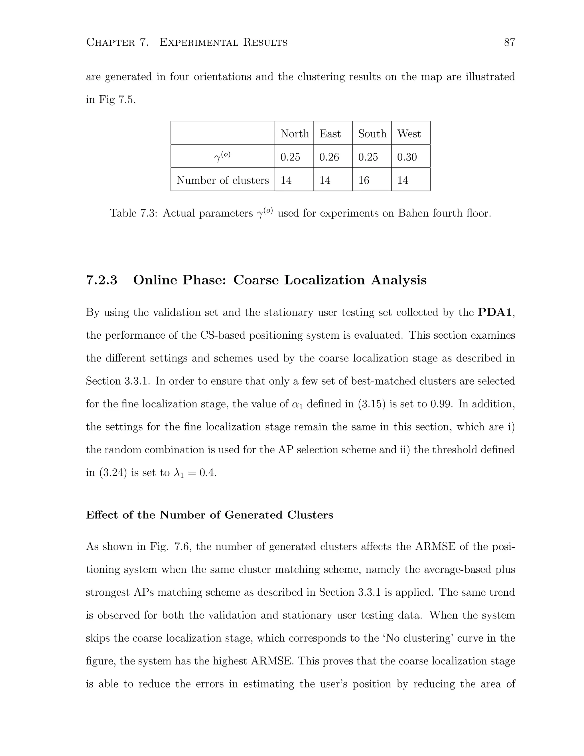
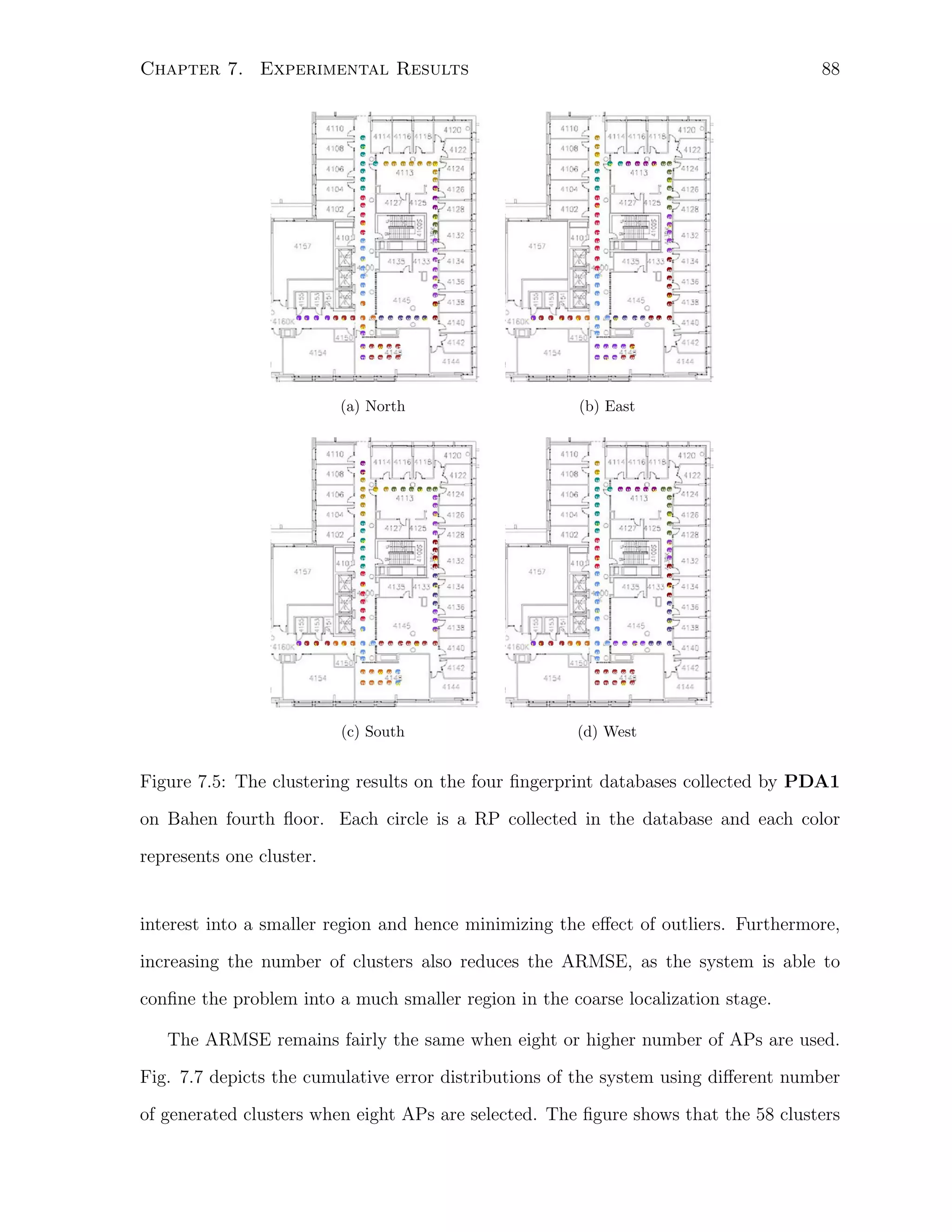
102. 89
Chapter 7. Experimental Results
used by the system achieve the best performance and attain the smallest maximum error.
Note that the error obtained from the stationary user testing set is slightly higher. This
is justified, as this set of data is collected on a different day and thus their RSS readings
are varied from the fingerprint database, introducing errors in estimations.
10
10
No clustering
No clustering
(o)
29 clusters; γ =1
9
9
29 clusters; γ(o)=1
8
43 clusters; γ(o)=0.5
58 clusters; actual clusters used by system
(o)
43 clusters; γ =0.5
58 clusters; actual clusters used by system
8
7
6
6
ARMSE [m]
ARMSE [m]
7
5
4
5
4
3
3
2
2
1
1
0
5
10
15
Number of APs Used
20
0
25
(a) Validation Data
5
10
15
Number of APs Used
20
25
(b) Stationary User Testing Data
Figure 7.6: The ARMSE versus number of used APs, when different number of generated
clusters are used for the coarse localization on Bahen fourth floor
0.9
0.8
0.8
Cumulative Error Probability
1
0.9
Cumulative Error Probability
1
0.7
0.6
0.5
0.4
No clustering
29 clusters; γ(o)=1
0.3
0.2
43 clusters; γ =0.5
58 clusters; actual clusters used by system
2
4
6
8
10
Distance Error [m]
12
(a) Validation Data
14
0.6
0.5
0.4
No clustering
29 clusters; γ(o)=1
0.3
(o)
0
0.7
16
0.2
43 clusters; γ(o)=0.5
58 clusters; actual clusters used by system
0
2
4
6
8
10
Distance Error [m]
12
14
16
(b) Stationary User Testing Data
Figure 7.7: The cumulative error distributions using different number of clusters for the
coarse localization on Bahen fourth floor. (8 APs are used)

103. 90
Chapter 7. Experimental Results
Different Matching Schemes
Section 3.3.1 describes several cluster matching schemes that can be used to select the
clusters, which best matched to the online RSS measurement vector r. Fig. 7.8 shows
the comparison of using different matching schemes. It is obvious that in the validation
set, the schemes that are applied on the strongest APs set have better accuracies and
they have similar performances, except that the exemplar-based scheme has a higher
maximum error. However, this trend is not as obvious as in the stationary user testing
set, as the gap between the schemes with and without the use of strongest APs set is very
small. In fact, the weighted average applied on the strongest APs set attains the highest
maximum error. According to both sets of data, the average based strongest APs cluster
matching scheme is a good choice for the system and is selected as the default operation
for the coarse localization stage as it gives reliable results in both sets.
1
0.9
0.8
0.8
Cumulative Error Probability
Cumulative Error Probability
1
0.9
0.7
0.6
0.5
Exemplar−based
Average−based
Weighted Average
Exemplar−based + Strongest APs
Average−based + Strongest APs
Weighted Average + Strongest APs
0.4
0.3
0.2
0
2
4
6
8
Distance Error [m]
10
0.7
0.6
0.5
Exemplar−based
Average−based
Weighted Average
Exemplar−based + Strongest APs
Average−based + Strongest APs
Weighted Average + Strongest APs
0.4
0.3
0.2
12
(a) Validation Data
0
2
4
6
8
Distance Error [m]
10
12
(b) Stationary User Testing Data
Figure 7.8: The cumulative error distributions using different cluster matching schemes
on Bahen fourth floor. (8 APs are used)
7.2.4
Online Phase: Fine Localization Analysis
This section focuses on the evaluation of using different settings for the fine localization
stage.

104. Chapter 7. Experimental Results
91
AP Selection Schemes
There are three access point selection schemes for the fine localization stage as described
in Section 3.3.2. The performances of using these schemes are compared in Fig. 7.9. For
the random combination AP selection scheme, the x-axis refers to the number of linear
random combinations of online RSS values from L APs according to (3.18). When the
number of used APs is less than 14, both the Fisher criterion and the random combination
AP selection schemes have similar results and achieve slightly better than the strongest
APs scheme. However, when the number used APs is higher than 14, the strongest APs
and Fisher criterion schemes achieve the same ARMSE in both sets of data, whereas,
the random combination results in a slightly higher ARMSE. Although the random combination may sometime leads to slightly higher ARMSE than the other two schemes,
it is chosen to be the default operation of the CS-based position system, as i) it does
not require large samples of RSS data for the calculations of variance as required by the
Fisher criterion; ii) it achieves better results when a small number of APs is used and iii)
the same random matrix Φ can be reused, unlike the other two online RSS schemes that
require on-the-fly generation of the AP selection matrix Φ and thus reduce the online
update time.
Sensitivity to Threshold λ1
Another parameter that is required to be determined experimentally is the threshold λ1
ˆ
defined in (3.24), as it determines how many non-zero entries of the θ should be used
to interpret the actual location of the user. Fig. 7.10 illustrates the effect of λ1 on
the ARMSE results. It shows that the ARMSE can vary for a range of 0.4m, which is
not very significant when comparing to the magnitude of the ARMSE, just by setting
a different value of λ1 . Although the value of λ1 does not have a linear relationship
to the ARMSE, the figures show that the λ1 should not be set to a high value, which
implies that the system only obtains a few entries with highest value for the location

105. 92
Chapter 7. Experimental Results
3.4
3.4
Strongs APs
Fisher Criterion
Random Combination
3.2
3
2.8
ARMSE [m]
3
2.8
ARMSE [m]
Strongs APs
Fisher Criterion
Random Combination
3.2
2.6
2.4
2.2
2.6
2.4
2.2
2
2
1.8
1.8
1.6
1.6
1.4
5
10
15
Number of APs Used
20
1.4
25
(a) Validation Data
5
10
15
Number of APs Used
20
25
(b) Stationary User Testing Data
Figure 7.9: The ARMSE versus number of used APs, using different AP schemes for fine
localization on Bahen fourth floor.
interpretation. According to this experiments, this threshold should be set to λ1 = 0.4
to let the system have the best performance.
2.2
2.1
2.1
ARMSE [m]
2.3
2.2
ARMSE [m]
2.3
2
1.9
2
1.9
1.8
1.8
1.7
1.7
1.6
0.3
1.6
0.4
0.5
0.6
λ1
0.7
0.8
0.9
(a) Validation Data
0.3
0.4
0.5
0.6
λ1
0.7
0.8
0.9
(b) Stationary User Testing Data
Figure 7.10: Effect of the threshold λ1 on ARMSE on Bahen fourth floor. (8 APs are
used)
7.2.5
Performance Comparison
Throughout the above experimentations, a set of optimal parameters that gives the best
performance of the CS-based positioning system can be determined and is given in Table

106. 93
Chapter 7. Experimental Results
7.4. The performance of this positioning system is then compared to the KNN and
kernel-based techniques in terms of the position error and computation time.
Total number of generated clusters
58
Coarse Localization - cluster matching scheme Average-based + Strongest APs
Coarse Localization - α1
Fine Localization - AP selection scheme
0.99
Random combination
Fine Localization - λ1
0.4
Number of APs used
8
Table 7.4: A set of optimal parameters for the CS-based position system applied on
Bahen fourth floor.
Position Error
The position errors of the three methods are compared in Fig. 7.11 in terms of their
cumulative error distributions. Table 7.5 and 7.6 summarize the statistics of their position
errors.
For validation set, the performance of the CS-based positioning system outperforms
the other two methods. It reduces the ARMSE by 0.45m (22%) and 0.30m (16%) over
the KNN and Kernel-based methods. In addition, the system also improves significantly
in terms of maximum error (46%) and variance (62%).
The position error is slightly higher for the stationary user testing set, as these RSSs
are collected on a different day. Although the improvement of the CS-based positioning
system is not significant in terms of ARMSE (4% for KNN and 12% for Kernel-based),
the system still outperforms the other two methods in terms of maximum errors and
variances.

107. 94
Chapter 7. Experimental Results
0.9
0.8
0.8
Cumulative Error Probability
1
0.9
Cumulative Error Probability
1
0.7
0.6
0.5
0.4
KNN
Kernel−based
CS−based Positioning
0.3
0.2
0
2
4
6
8
10
Distance Error [m]
12
14
0.7
0.6
0.5
0.4
KNN
Kernel−based
CS−based Positioning
0.3
16
(a) Validation Data
0.2
0
2
4
6
8
10
Distance Error [m]
12
14
16
(b) Stationary User Testing Data
Figure 7.11: The cumulative error distributions using different positioning systems on
Bahen fourth floor. (8 APs are used)
Method
ARMSE [m]
Mean [m]
90th Percentile [m]
Max[m] Variance [m2 ]
KNN
2.02
1.78
3.15
17.3
5.74
Kernel-based
1.87
1.56
3.78
13.39
3.99
CS-based
1.57
1.29
2.84
7.19
1.51
Table 7.5: Position error statistics for different methods on Bahen fourth floor. (For
validation set)
Method
ARMSE [m]
Mean [m]
90th Percentile [m]
Max[m] Variance [m2 ]
KNN
2.00
1.76
3.39
8.35
2.51
Kernel-based
2.19
1.86
3.81
10.54
3.81
CS-based
1.92
1.67
3.38
7.16
1.76
Table 7.6: Position error statistics for different methods on Bahen fourth floor. (For
stationary user testing set)
Computation Time
R
Fig. 7.12 shows the computation time required for each step on a 2.50GHz Intel⃝ Core
TM
2 Quad processor with 4GB RAM using the three different localization techniques. Since

108. 95
Chapter 7. Experimental Results
the Kernel-based method is a probabilistic approach that incorporates all RSS time
samples from the fingerprint database for computation, it requires much more time to
obtain the estimated position than the other two methods. Its computation time also
increases as the number of used APs increases. Due to its high-volume computation cost,
it is not desirable to implement on the resource-limited mobile devices as a real-time
positioning system. Although the CS-based system requires a little more computation
time than the KNN method, its simplicity and accuracy makes it a good method to be
implemented on any mobile device.
0.03
0.025
0.025
Mean Computation Time [s]
0.035
0.03
Mean Computation Time [s]
0.035
0.02
KNN
Kernel−based
CS−based Positioning
0.015
0.02
KNN
Kernel−based
CS−based Positioning
0.015
0.01
0.01
0.005
0.005
0
4
6
8
10
12
14
16
Number of APs Used
18
20
22
24
(a) Validation Data
26
0
4
6
8
10
12
14
16
Number of APs Used
18
20
22
24
26
(b) Stationary User Testing Data
Figure 7.12: Comparison of mean computation time using different positioning systems
in Bahen fourth floor. (8 APs are used)
7.3
Tracking Results on CNIB Second Floor
In this section, the performance of the proposed tracking system described in Chapter 4
is evaluated based on the RSS data collected by the PDA2 device on the second floor of
CNIB.

109. Chapter 7. Experimental Results
7.3.1
96
RSS Distributions
The RSS distributions based on the three sets of fingerprint databases collected by
PDA1, PDA2 and Smartphone are examined briefly in this section. Fig. 7.13, 7.14
and 7.15 show the RSS distributions in terms of different parameters for all the three
devices. Several observations can be made from these figures:
• There are some instances during the RSS sampling period that PDA1 and Smartphone are not able to detect the RSS from certain APs, thus their fingerprint
databases are degraded.
• Although the RSS collected by PDA1 is the strongest, its RSS distribution in
spatial domain fluctuates significantly when comparing to the other two devices as
shown in Fig. 7.15b. This large fluctuation is undesirable as it introduces error to
the positioning system.
• The RSS collected by Smartphone is significantly lower than the other two methods, as the device’s antenna is of poor quality.
• The fingerprint database collected by PDA2 is the most stable over all the three
devices and thus is used by the proposed tracking analysis for the following sections.
7.3.2
CS-based Positioning Results
Before the analysis of the tracking system, the original CS-based positioning system is
first compared to the KNN and Kernel-based methods. The generated cluster results
after the modification of outliers are shown in 7.16 and the optimal set of parameters
used by the system is summarized in Table 7.7.
Fig. 7.17 and Table 7.8 compare the performances of the three localization methods
on the mobile user testing set. The CS-based method behaves slightly worse than the
KNN method unlike the results obtained for the Bahen fourth floor. This happens as a

110. 97
Chapter 7. Experimental Results
12
6
10
5
8
10
4
9
8
7
5
Frequency
Frequency
Frequency
6
6
3
4
4
2
2
1
3
2
1
0
−120
−110
−100
−90
−80
−70
RSS Readings [dBm]
−60
−50
−40
(a) RSS collected by PDA1
0
−66
−65
−64
−63
−62 −61 −60 −59
RSS Readings [dBm]
−58
−57
0
−120
−56
−110
−100
−90
RSS Readings [dBm]
−80
−70
−60
(b) RSS collected by PDA2 (c) RSS collected by Smartphone
Figure 7.13: Example histograms of RSS distributions of the same access point over
50 time samples (40 time samples for Smartphone) for different devices at the same
reference point in CNIB second floor.
−45
−40
PDA1 − North
PDA2 − North
Smartphone − North
−50
−50
−55
RSS Average [dBm]
RSS readings [dBm]
−60
−70
−80
−60
−65
−70
−90
−110
−75
PDA1 − North
PDA2 − North
Smartphone − North
−100
−80
0
5
10
15
20
25
Time [s]
30
35
40
45
(a) RSS distributions across time
50
−85
0
5
10
15
20
25
30
Number of RSS time samples
35
40
45
50
(b) RSS averages across time samples
Figure 7.14: An example of RSS distributions across time and their averages with respect
to the number of time samples of the same access point for different devices at the same
reference point in CNIB second floor.
part of the CNIB second floor does not have a good coverage of the APs, which leads
to poor clustering results around that region and makes the system hard to identify the
correct clusters during the coarse localization stage. This also explains why the system
attains very high maximum error, as it selects the wrong regions for localization. This
effect is less prominent for the KNN method, as it compares the online RSS measurement

111. 98
Chapter 7. Experimental Results
−40
−40
PDA2 − North
PDA2 − South
PDA1 − North
PDA2 − North
Smartphone − North
−60
RSS Readings [dBm]
−50
−60
RSS Readings [dBm]
−50
−70
−80
−70
−80
−90
−90
−100
−100
−110
0
5
10
15
Reference Points Indices
20
25
(a) Different Orientations
30
−110
0
5
10
15
Reference Points Indices
20
25
30
(b) Different Devices
Figure 7.15: An example of RSS distributions of the same access point in spatial domain
for different orientations and different devices in CNIB second floor. (only a part of the
fingerprints are shown)
(a) North (11 Generated Clusters)
(b) East (17 Generated Clusters)
(c) South (15 Generated Clusters)
(d) West (16 Generated Clusters)
Figure 7.16: The clustering results on the four fingerprint databases collected by PDA2
on CNIB second floor
readings to each of the RP’s RSS values instead of a subset of them.
The proposed tracking system described in Chapter 4 is able to improve the CS-

112. 99
Chapter 7. Experimental Results
Total number of generated clusters
59
Coarse Localization - cluster matching scheme Average-based + Strongest APs
Coarse Localization - α1
0.99
Fine Localization - AP selection scheme
Random combination
Fine Localization - λ1
0.4
Number of APs used
10
Table 7.7: A set of optimal parameters for the CS-based position system applied on
CNIB second floor.
based positioning system by using previous history to ensure it chooses the correct relevant region during the coarse localization stage and smooths out the trajectory by the
application of the Kalman filter. Their analysis are in the following sections.
1
0.9
Cumulative Error Probability
0.8
0.7
0.6
0.5
0.4
0.3
0.2
KNN
Kernel−based
CS−based
0.1
0
0
2
4
6
8
10
12
Distance Error [m]
14
16
18
Figure 7.17: The cumulative error distributions for different positioning systems on CNIB
second floor. (10 APs are used)
7.3.3
Modified Coarse Localization Analysis
In this section, the use of different schemes to choose the RPs which are in physical proximity to the previous estimate, described in Section 4.3.1, are examined. The covariances

113. 100
Chapter 7. Experimental Results
Method
ARMSE [m]
Mean [m]
90th Percentile [m]
Max[m] Variance [m2 ]
KNN
3.02
2.56
4.84
16.55
3.49
Kernel-based
3.73
3.06
6.24
15.30
6.31
CS-based
3.28
2.68
5.26
26.64
4.79
Table 7.8: Positioning error statistics for different positioning methods on CNIB second
floor. (For mobile user testing set)
of the process and measurement noises of the Kalman filter are set to S = diag(1) and
U = diag(80), where diag(d) refers to a diagonal matrix with the diagonal entries set to
the scalar value d.
According to Section 4.3.1, there are two parameters to be set for choosing the relevant
RPs depending on their geographical locations to the previous user’s location. The first
parameter is to decide whether the previous estimated location (Unpredicted ) should be
used for the distance calculations to the RPs or the predicted location using the Kalman
filter estimated state vector (Predicted ) should be used. The second parameter is the
walking distance range β defined in (4.15) and (4.17).
Fig. 7.18 shows the ARMSE versus the walking distance range β when different
schemes are used. Both schemes work the best when β = 4. In addition, the Unpredicted
one works better than the Predicted one. This happens as the Predicted scheme may
not be able to predict the correct user’s current location and thus introduce errors when
including non-relevant RPs for the fine localization stage.
7.3.4
Map Adaptive Kalman Filter Analysis
In this section, the unpredicted user’s location and β = 0.4 are used for the coarse
localization stage and different parameters for the Kalman filter are examined.

114. 101
Chapter 7. Experimental Results
2.9
2.8
Unpredicted
Predicted
2.7
ARMSE [m]
2.6
2.5
2.4
2.3
2.2
2.1
2
3
3.5
4
4.5
β [m]
5
5.5
6
Figure 7.18: Effect of the walking distance β on ARMSE in CNIB second floor. (10 APs
are used)
Sensitivity to the Covariances of Process and Measurement Noises.
Fig. 7.19 illustrates the performances of the proposed tracking system using different
combinations of covariances of process and measurement noises, S = diag(ds) and U =
diag(du), respectively. The performances are very similar for most of the combinations,
except for the case when ds = 10 and du = 80. It shows that the performance of the
proposed tracking system is not affected significantly by changing the parameters of the
Kalman filter.
1
0.9
Cumulative Error Probability
0.8
0.7
0.6
0.5
0.4
0.3
ds = 1, du = 80
ds = 1, du = 100
ds = 1, du = 50
ds = 10, du = 80
ds = 0.5, du = 80
0.2
0.1
0
0
2
4
6
Distance Error [m]
8
10
12
Figure 7.19: The cumulative error distributions using different Kalman filter parameters
in CNIB second floor. (10 APs are used)

115. 102
Chapter 7. Experimental Results
Resetting Kalman Filter at Intersections
Section 4.3.2 mentions that the Kalman filter should be reset at the intersections, where
there are a higher chance for the user to make turns and thus violate the linear motion
model assumed by the Kalman filter. Fig. 7.19 compares the performance with and
without resetting the Kalman filter at the intersections. Resetting the Kalman filter
at intersections improves the system’s accuracy. For the ARMSE, the resetting scheme
improves from 2.20m to 2.07m (6%) and at the 90th percentile, it improves from 3.76m
to 3.33m (11%).
1
0.9
Cumulative Error Probability
0.8
0.7
0.6
0.5
0.4
0.3
0.2
0.1
0
No reset Kalman filter at corner
Reset Kalman filter at corner
0
2
4
6
Distance Error [m]
8
10
12
Figure 7.20: The cumulative error distributions for different Kalman filter update schemes
in CNIB second floor. (10 APs are used)
7.3.5
Performance Comparison
From the above analysis, a set of optimal parameters that gives the best performance for
the proposed tracking system is shown in Table 7.9. This tracking system is compared
with the original CS-based positioning system and the direct applications of the Kalman
filter on both the KNN method and the CS-based positioning system. Fig. 7.21 shows the
comparison results in terms of cumulative error distributions and Table 7.10 shows the
position error statistics for these four systems. The proposed tracking system outperforms

116. 103
Chapter 7. Experimental Results
the other three methods. It reduces the ARMSE by 1.27m (39%), 0.64m (27%) and 0.53m
(21%) over the CS-based positioning system, the KNN method with the Kalman filter
and the CS-based position system with the Kalman filter, respectively. In addition, the
proposed tracking system also has the smallest 90th percentile error and variance when
compared to the other systems.
Modified Coarse Localization - Comparison schemes
Non-Prediction scheme
Modified Coarse Localization - β
4m
Kalman Filter Covariances
S = diag(1) U = diag(80)
Table 7.9: A set of optimal parameters for the proposed tracking system applied on CNIB
second floor.
1
0.9
0.8
Cumulative Error Probability
0.7
0.6
0.5
0.4
0.3
0.2
CS−based
KNN + Kalman Filter
CS−based + Kalman Filter
Proposed Tracking
0.1
0
0
2
4
6
Distance Error [m]
8
10
12
Figure 7.21: The cumulative error distributions using the CS-based positioning system
and the three tracking systems in CNIB second floor. (10 APs are used)
Some of the example trace results are shown in Fig. 7.22. The estimated traces by the
proposed tracking system are able to follow the actual traces walked by the user. These
traces certainly improve the locations estimated by the CS-based positioning system
shown as green dots on the figures.

117. 104
Chapter 7. Experimental Results
Method
ARMSE [m]
Mean [m]
90th Percentile [m]
Max [m] Var [m2 ]
CS-based Positioning
3.28
2.68
5.26
26.64
4.79
KNN +
2.75
2.41
4.41
10.95
2.42
2.54
2.17
4.15
24.10
2.69
2.01
1.74
3.36
17.93
1.91
Kalman Filter
CS-based +
Kalman Filter
Proposed Tracking
Table 7.10: Position error statistics for the CS-based positioning system and the two
tracking systems on CNIB second floor. (For mobile user testing set)
(a) Trace #1
(b) Trace #2
(c) Trace #3
(d) Trace #4
Figure 7.22: Example trace results. The black line is the actual trace, the green dots
are the CS-based positioning results and the purple line is the results of the proposed
tracking system.
7.3.6
Navigation and Real Time Implementations
Using the PDA2, which is installed with the developed software that implemented the
proposed positioning and tracking system as described in Chapter 6, the user is able to

118. Chapter 7. Experimental Results
105
obtain the real-time estimated position updates periodically from the device. In addition,
the user is able to use the navigation function provided by the software.
The navigation module of the software requires the input of the map database, which
helps the module to generate useful guidance to the user according to his locations. Fig.
7.23 depicts the definition of the connected graph and the map features on CNIB second
floor, which are obtained according to Section 5.2.
Figure 7.23: The definition of the connected graph and the map features on CNIB second
floor. The blue lines and blue circles represent the edges and nodes of the connected
graph. The red squares represents the destinations. The diamonds represents the map
features and the pink circles represents the locations of the 15 deployed access points
At the beginning of the navigation, the device asks the user to enter the desired target
and then the module will route the path and play appropriate audio files to ask the user
to follow the path. The actual operations of the navigation can be found in Chapter 5.
Fig. 7.24 shows an example screenshot that is obtained from the device at the end of the
real experiment carried on the CNIB second floor. The device is able to track the user’s
trajectory and give appropriate commands accordingly. Several video files can be found
online in [85] to show the actual experiments conducted on CNIB second floor.

119. Chapter 7. Experimental Results
106
Figure 7.24: Example screenshot of the software that shows the actual track that the
user is walking. The line shows the routed path generated by the navigation module.
The squares denote the user’s locations and the circle denotes the destination.
7.3.7
Subject Testing
A preliminary research study was conducted over two months (in July and August 2010)
at this site in collaboration with the CNIB research unit to evaluate if such navigation
software developed on the smart device is useful in providing guidance to people with low
vision, as defined according to [86]. Before the actual testing, the subject’s visual acuity
was first examined by a doctor for low vision. A total of 16 visually impaired subjects
with an average age of 55 took part in this study and they were randomly assigned
into two groups, each group contains 8 subjects: i) subjects in the Control group were
only given instructions at the beginning of the test to reach the target by themselves;
whereas ii) subjects in the Testing group were given the PDA2, which provided real-time
navigation to guide them to the target. Each subject carried either a mobility cane or a
guide dog and was required to walk three pre-determined paths, which are the same as
the first three testing traces in the mobile user testing data. Table 7.11 gives a summary
about these traces. The results of this study are summarized in Table 7.12. Successful
trial means that the subject is able to reach the destination at the end of the test.
Several observations can be made according to the results in Table 7.12:
• The Testing group has a higher successful rate than the Control group. Since the

120. 107
Chapter 7. Experimental Results
Trace
Start Position
Destination
# of Turns
Distance
1 (Fig. 7.22a)
Rm 207
Rm 218E
2
53.63m
2 (Fig. 7.22b)
Rm 218E
Spring Water Fountain
2
29.43m
3 (Fig. 7.22c)
Spring Water Fountain
Elevator
0
30.80m
Table 7.11: Summary of the three traces tested by the subjects
Trace
Group
Number of successful
Average Elapsed Time
trials (out of 8)
(for successful trials)
1
Control
4
180.3 s
1
Testing
6
252.4 s
2
Control
3
83.3 s
2
Testing
8
130.5 s
3
Control
7
76.4 s
3
Testing
8
97.5 s
Table 7.12: Subjects testing results on CNIB second floor
device is able to identify the user’s location and informs that the subject has reached
the destination, the users are able to stop accordingly. However, the users from the
Control group have no extra assistance in identifying the destinations except the
instructions given at the beginning, thus they have to rely on their limited visions
to identify the targets and have difficulties to stop at the correct destinations. This
is especially obvious for the second trace, as the target is a spring water fountain,
which is small and is easy to be missed by the subjects.
• The time required for the subjects from the Testing group to reach the destinations
is longer than the one required for the Control group. This happens because of
two reasons. First, since the device generates additional descriptive instructions

121. Chapter 7. Experimental Results
108
about the surrounding area, the users spend extra time to get familiar with the
building. Second reason is due to hardware limitations of the PDA2. The slow
response of the WiFi network adaptor of the PDA2 and the duration time to play
the instructions lead to the slow actual update rate of the tracking system. Hence,
the subjects are required to walk slowly to accommodate these limitations.
This study shows positive results that the navigation software is useful to give realtime guidance to the visually impaired people. However, further research is required to
improve the actual tracking rate of the system. This may be done by using a different
device that has a better processor, memory or WiFi network adaptor than PDA2.
7.4
Chapter Summary
This chapter evaluates the performances of the proposed CS-based positioning and tracking system. There are two experimental sites. The experiments carried on the fourth
floor of Bahen Centre focus on the analysis of the CS-based positioning system, whereas
the analysis of the proposed tracking system is done on second floor of the CNIB. The
CS-based positioning system outperforms the KNN and kernel-based methods on the Bahen fourth floor and the proposed tracking system is able to further improve the accuracy
in estimating the user’s locations on the CNIB second floor. This lightweight algorithm
can be implemented as a software on the resource-limited mobile devices, such as PDAs
and smartphones. Furthermore, a simple navigation module is included and the real-time
performance can be found in [85].

122. Chapter 8
Conclusion
In this thesis, a RSS-based WLAN indoor positioning system, which can be implemented
on resource-limited mobile devices, is proposed. It is a fingerprint-based localization
system, which an offline phase, also known as a training phase, is required to collect the
RSS readings from access points (APs) at known positions, referred to as the reference
points (RPs). Unlike the probabilistic methods, which incorporate each individual RSS
time samples collected in the database for computation of the position estimate, the
proposed system uses only the averages of those RSS samples and perhaps their variances
depending on the choice of AP selection scheme. Thus, its computation complexity is
much less than the probabilistic methods and can be implemented on the mobile devices
without exhausting their computation powers. After the fingerprint database collection is
done, a clustering process is carried on to group the RPs with similar RSS values together
by applying the affinity propagation algorithm. The cluster members in the same cluster
should also be geographically close to each other and the outliers are manually assigned
back to the clusters that are physically close to them. The proposed positioning system
contains two stages for the actual positioning that happens in the online phase. First, the
coarse localization stage confines the localization problem into a smaller relevant region
by choosing the clusters of RPs, which are most similar to the online RSS measurement
109

123. Chapter 8. Conclusion
110
values. Then, the fine localization stage translates the fingerprint-based localization
problem into a sparse-signal recovery problem, so that the compressive sensing (CS)
theory can be applied and the user’s location can be estimated by solving a ℓ1 norm
minimization problem.
This CS-based positioning system can be easily extended to improve the accuracy by
using the previous estimate to refine the position estimates. First, the tracking system
uses the previous position estimate, in addition to the online RSS values to select the
subset of relevant RPs in the coarse localization stage. Second, the Kalman filter is used
to post-process the estimate computed at the end of fine localization stage to obtain
the final estimate. Resetting the Kalman filter when the location estimate is within a
intersection region helps to improve the accuracy, as the user is more likely to make
turns at intersections and thus violates the linear motion model assumed by the Kalman
filter. The tracking system is able to provide real-time estimates on the resource limited
devices, as the computation cost for the Kalman filter is very low when comparing to the
particle filter.
The proposed position and tracking system is implemented as a software which can
be installed on any Windows Mobile based handheld devices. The performance of the
proposed positioning and tracking system is evaluated in two different experimental sites:
fourth floor of Bahen centre and second floor of CNIB, where the RSS readings are
collected by two different PDAs. Experimental results show that the CS-based positioning
system performs better than the KNN and kernel-based methods on the Bahen fourth
floor in terms of average, maximum and 90th percentile errors, whereas on the CNIB
second floor, the proposed tracking system is able to further improve the accuracy in
estimating the user’s locations.
Finally, the simple navigation system is also implemented on top of the proposed
tracking system on the software. This software installed on the PDA was tested by
several visually impaired subjects on the second floor of CNIB. Results from this study

124. Chapter 8. Conclusion
111
show that the system is able to track the users’ trajectories properly and give useful
guidance.
8.1
Future Works
There are several problems that can be explored to further enhance the performance of
the proposed WLAN positioning and tracking system. They are listed as follow:
• Besides the WiFi adapter, most of the smartphones and PDAs are now equipped
with extra sensors, such as accelerometer and digital compass. The information
generated from these sensors can be interpreted as user’s walking distances and
orientations. Although the samsung smartphone evaluated in this thesis is incompetent to handle the WiFi scanning and the operations of the sensors together,
recent smartphones are equipped with higher performance processor [87] and may
allow the sensors to be used in conjunction to the WLAN positioning system.
Thus, the proposed positioning system should be extended to use the information
obtained from these sensors to improve the accuracy of the estimated position.
• One of the disadvantages of using a fingerprinting based methods is the high labour
and time cost for collecting the required fingerprint database during the offline
phase. Since the fingerprints can be considered sparse in terms of the spatial
domain for the whole region of interest, the compressive sensing theory may be
applied on a smaller set of RPs to produce a larger radio map to reduce the time
to collect the fingerprints.
• In addition to using the CS theory to reduce the number of fingerprints, empirical
indoor radio propagation models may be used in conjunction to the fingerprinting
process to interpolate the RSS of extra RPs based on a small set of fingerprints, as
Fig. 7.3 and Fig. 7.15 show that the signal strength varies smoothly over spatial

125. Chapter 8. Conclusion
112
domain.
• The proposed positioning system is device-dependent, thus the fingerprinting process must be done for each different mobile devices. Recent studies show that using
signal strength differences (SSD) between pairs of APs instead of RSS can improve
the accuracy of the position estimate when different devices are used in a small
region [33]. Thus, research and analysis can be done to evaluate if the proposed
positioning system can use the SSD as the measurement metric.

126. Bibliography
[1] K. W. Kolodziej and J. Hjelm, Local Positioning Systems: LBS Applications and
Services. Taylor & Francis Group, 2006.
[2] A. Kushki, K. N. Plataniotis, and A. N. Venetsanopoulos, “Kernel-Based Positioning
in Wireless Local Area Networks,” Mobile Computing, IEEE Transactions on, vol. 6,
no. 6, pp. 689 –705, June 2007.
[3] A. Brimicombe and C. Li, Location-Based Services and Geo-Information Engineering. Wiley-Blackwell, 2009.
[4] M. Rodriguez, J. Favela, E. Martinez, and M. Munoz, “Location-Aware Access
to Hospital Information and Services,” IEEE Trans. Information Technology in
Biomedicine, vol. 8, no. 4, pp. 448–455, 2004.
[5] P. Thornycroft, “Location-based services for cellular phones using Wi-Fi: The University of Cincinnati’s system for emergency call location,” University of Cincinnati,
White Paper, 2009.
[6] A. LaMarca and E. de Lara, Location Systems: An Introduction to the Technology Behind Location Awareness, ser. Synthesis Lectures on Mobile and Pervasive
Computing. Morgan and Claypool Publishers, 2008.
113

127. 114
Bibliography
[7] G. Sun, J. Chen, W. Guo, and K. J. R. Liu, “Signal Processing Techniques in
Network-Aided Positioning: A Survey of State-of-the-art Positioning Designs,”
IEEE Signal Processing Magazine, vol. 22, no. 4, pp. 12–23, 2005.
[8] H. Liu, H. Darabi, P. Nanerjee, and J. Liu, “Survery of Wireless Indoor Positioning
Techniques and Systems,” IEEE Transactions on Systems, Man and CyberneticsPart C: Applications and Reviews, vol. 37, no. 6, pp. 1067–1080, Novermber 2007.
[9] A. Varshavsky, D. Pankratov, J. Krumm, and E. de Lara, “Calibree: Calibration-free
localization using relative distance estimations,” in Sixth International Conference
on Pervasive Computing (Pervasive), Sydney, Australia, May 2008.
[10] A. Varshavsky, E. de Lara, J. Hightower, A. LaMarca, and V. Otsason, “GSM Indoor
Localization,” Pervasive and Mobile Computing Journal (PMC), vol. 3, no. 6, pp.
698–720, December 2007.
[11] W. ur Rehman, E. de Lara, and S. Saroiu, “CILoS: A CDMA Indoor Localization
System,” in 10th International Conference on Ubiquitous Computing (Ubicomp),
Seoul, South Korea, September 2008.
[12] R. Mautz, “The challenges of indoor environments and specification on some alternative positioning systems,” in Positioning, Navigation and Communication, 2009.
WPNC 2009. 6th Workshop on, March 2009, pp. 29 –36.
[13] L. Jing, P. Liang, C. Maoyong, and S. Nongliang, “Super-resolution time of arrival
estimation for indoor geolocation based on IEEE 802.11 a/g,” in Intelligent Control
and Automation, 2008. WCICA 2008. 7th World Congress on, June 2008, pp. 6612
–6615.
[14] “Aeroscout company.” [Online]. Available:
difference
http://www.aeroscout.com/content/

128. 115
Bibliography
[15] B. J. Frey and D. Dueck,
“Clustering by Passing Messages Between
Data Points,” Science, vol. 315, pp. 972–976, 2007. [Online]. Available:
www.psi.toronto.edu/affinitypropagation
[16] E. J. Cand`s and M. B. Wakin, “An introduction to compressive sampling,” IEEE
e
Signal Processing Magazine, vol. 25, no. 2, pp. 21–30, March 2008.
[17] J. Hightower and G. Borriello, “Location systems for ubiquitous computing,” Computer, vol. 34, no. 8, pp. 57 –66, August 2001.
[18] “Ekahau Real Time Location System (RTLS) Overview,” 2010. [Online]. Available:
http://www.ekahau.com/products/real-time-location-system/overview.html
[19] P. Bahl and V. N. Padmanabhan, “RADAR: an in-building RF-based user location
and tracking system,” in INFOCOM 2000. Nineteenth Annual Joint Conference of
the IEEE Computer and Communications Societies. Proceedings. IEEE, vol. 2, 2000,
pp. 775 –784.
[20] ——, “Enhancements to the RADAR User Location and Tracking System,” Microsoft Research, Tech. Rep., February 2000.
[21] “Place lab:
A privacy-observant location system.” [Online]. Available:
http:
//www.placelab.org/
[22] K. Kaemarungsi and P. Krishnamurthy, “Properties of indoor received signal
strength for wlan location fingerprinting,” in Mobile and Ubiquitous Systems: Networking and Services, 2004. MOBIQUITOUS 2004. The First Annual International
Conference on, aug. 2004, pp. 14 – 23.
[23] C. Feng, W. S. A. Au, S. Valaee, and Z. Tan, “Compressive Sensing Based Positioning Using RSS of WLAN Access Points,” in INFOCOM, 2010 Proceedings IEEE,
March 2010, pp. 1 –9.

129. Bibliography
116
[24] ——, “Orientation-aware indoor localization using affinity propagation and compressive sensing,” in Computational Advances in Multi-Sensor Adaptive Processing
(CAMSAP), 2009 3rd IEEE International Workshop on, December 2009, pp. 261
–264.
[25] A. Bensky, Wireless Positioning Technologies and Applications. Artech House, Inc.,
2008.
[26] R. Singh, L. Macchi, C. Regazzoni, and K. Plataniotis, “A statistical modelling
based location determination method using fusion in WLAN,” in Proceedings of the
International Workshop on Wireless Ad-hoc Networks, 2005.
[27] N. K. Sharma, “A weighted center of mass based trilateration approach for locating
wireless devices in indoor environment,” in Proceedings of the 4th ACM international
workship on Mobility management and wireless access, 2006, pp. 112–115.
[28] K. Kaemarungsi and P. Krishnamurthy, “Modeling of indoor positioning systems
based on location fingerprinting,” in INFOCOM 2004. Twenty-third AnnualJoint
Conference of the IEEE Computer and Communications Societies, vol. 2, March
2004, pp. 1012 – 1022 vol.2.
[29] A. Goldsmith, Wireless Communications, 1st ed. Cambridge University Press, 2005.
[30] B. Li, Y. Wang, H. K. Lee, A. Dempster, and C. Rizos, “Method for yielding a
database of location fingerprints in WLAN,” Communications, IEEE Proceedings-,
vol. 152, no. 5, pp. 580 – 586, October 2005.
[31] J. Yin, Q. Yang, and L. M. Ni, “Learning Adaptive Temporal Radio Maps for SignalStrength-Based Location Estimation,” Mobile Computing, IEEE Transactions on,
vol. 7, no. 7, pp. 869 –883, July 2008.

130. Bibliography
117
[32] K. Kaemarungsi, “Distribution of WLAN received signal strength indication for
indoor location determination,” in Wireless Pervasive Computing, 2006 1st International Symposium on, January 2006, p. 6 pp.
[33] A. K. M. Mahtab Hossain, H. N. Van, Y. Jin, and W.-S. Soh, “Indoor Localization
Using Multiple Wireless Technologies,” in Mobile Adhoc and Sensor Systems, 2007.
MASS 2007. IEEE Internatonal Conference on, October 2007, pp. 1 –8.
[34] V. Honkavirta, T. Perala, S. Ali-Loytty, and R. Piche, “A comparative survey of
WLAN location fingerprinting methods,” in Positioning, Navigation and Communication, 2009. WPNC 2009. 6th Workshop on, March 2009, pp. 243 –251.
[35] B. Li, J. Salter, A. G. Dempster, and C. Rizos, “Indoor positioning techniques based
on wireless lan,” in 1st IEEE Internal Conference on Wireless Broadband & Ultra
Wideband Communications, March 2006, pp. 13–16.
[36] M. Youssef and A. Agrawala, “The Horus WLAN location determination system,”
in MobiSys ’05: Proceedings of the 3rd international conference on Mobile systems,
applications, and services. New York, NY, USA: ACM, 2005, pp. 205–218.
[37] T. Roos, P. Myllym¨ki, H. Tirri, P. Misikangas, and J. Siev¨nen, “A Probabilistic
a
a
Approach to WLAN User Location Estimation,” Internation Journal of Wireless
Information Networks, vol. 9, no. 3, pp. 155–164, July 2002.
[38] A. Kushki, “A Cognitive Radio Tracking System for Indoor Environments,” Ph.D.
dissertation, University of Toronto, 2008.
[39] M. Youssef, A. Agrawala, and A. U. Shankare, “WLAN Location Determination via
Clustering and Probability Distributions,” in Proc, First IEEE Int’l Conf, Pervasive
Computing and Comm, 2003, pp. 143–155.

131. Bibliography
118
[40] Y. Chen, Q. Yang, J. Yin, and X. Chai, “Power-Efficient Access-Point Selection
for Indoor Location Estimation,” IEEE Transactions on Knowledge and Data Engineering, vol. 19, no. 7, pp. 877–888, July 2006.
[41] I. Guvenc, C. T. Abdallah, R. Jordan, and O. Dedeoglu, “Enhancements to RSS
Based Indoor Tracking Systems Using Kalman Filters,” in Global Signal Processing
Expo and International Signal Processing Conference, 2003.
[42] J. A. Besada, A. M. Bernardos, P. Tarrio, and J. R. Casar, “Analysis of tracking
methods for wireless indoor localization,” in Wireless Pervasive Computing, 2007.
ISWPC ’07. 2nd International Symposium on, February 2007.
[43] A. Kushki, K. N. Plataniotis, and A. N. Venetsanopoulos, “Location Tracking in
Wireless Local Area Networks with Adaptive Radio MAPS,” in Acoustics, Speech
and Signal Processing, 2006. ICASSP 2006 Proceedings. 2006 IEEE International
Conference on, vol. 5, May 2006, pp. V –V.
[44] F. Evennou and F. Marx, “Improving positioning capabilities for indoor environments with Wifi,” in IST Summit, 2005.
[45] J. Yim, S. Jeong, J. Joo, and C. Park, “Utilizing Map Information for WLANBased Kalman Filter Indoor Tracking,” in Future Generation Communication and
Networking Symposia, 2008. FGCNS ’08. Second International Conference on, vol. 5,
December 2008, pp. 58 –62.
[46] Y. Song and H. Yu, “A RSS Based Indoor Tracking Algorithm via Particle Filter
and Probability Distribution,” in Wireless Communications, Networking and Mobile
Computing, 2008. WiCOM ’08. 4th International Conference on, October 2008, pp.
1 –4.

132. Bibliography
119
[47] M. S. Arlampalam, S. Maskell, N. Gordon, and T. Clapp, “A Tutorial on Particle
Filters for Online Nonlinear/NonGaussian Bayesain Tracking,” IEEE Transactions
on Signal Processing, vol. 50, no. 2, pp. 174–188, February 2002.
[48] H. Wang, H. Lenz, A. Szabo, J. Bamberger, and U. D. Hanebeck, “Enhancing
the map usage for indoor location-aware systems,” in HCI’07: Proceedings of the
12th international conference on Human-computer interaction. Berlin, Heidelberg:
Springer-Verlag, 2007, pp. 151–160.
[49] C.-H. Chao, C.-Y. Chu, and A.-Y. Wu, “Location-Constrained Particle Filter human
positioning and tracking system,” in Signal Processing Systems, 2008. SiPS 2008.
IEEE Workshop on, October 2008, pp. 73 –76.
[50] Widyawan, M. Klepal, and S. Beauregard, “A novel backtracking particle filter
for pattern matching indoor localization,” in MELT ’08: Proceedings of the first
ACM international workshop on Mobile entity localization and tracking in GPS-less
environments. New York, NY, USA: ACM, 2008, pp. 79–84.
[51] H. Wang, H. Lenz, A. Szabo, J. Bamberger, and U. Hanebeck, “WLAN-Based Pedestrian Tracking Using Particle Filters and Low-Cost MEMS Sensors,” in Positioning,
Navigation and Communication, 2007. WPNC ’07. 4th Workshop on, March 2007,
pp. 1 –7.
[52] O. Woodman and R. Harle, “Pedestrian localisation for indoor environments,” in
UbiComp ’08: Proceedings of the 10th international conference on Ubiquitous computing. New York, NY, USA: ACM, 2008, pp. 114–123.
[53] I.-E. Liao and K.-F. Kao, “Enhancing the accuracy of WLAN-based location determination systems using predicted orientation information,” Inf. Sci., vol. 178, no. 4,
pp. 1049–1068, 2008.

133. Bibliography
120
[54] R. Zhou, “Wireless Indoor Tracking System (WITS),” in doIT Conference on Software Research, 2006, pp. 163–177.
[55] A. Kushki, K. N. Plataniotis, and A. N. Venetsanopoulos, “Intelligent Dynamic
Radio Tracking in Indoor Wireless Local Area Networks,” Mobile Computing, IEEE
Transactions on, vol. 9, no. 3, pp. 405 –419, March 2010.
[56] P.-Y. Gilli´ron and B. Merminod, “Personal Navigation System for Indoor Applicae
tions,” in Proceedings of the 11th IAIN World Congress, 2003.
[57] A. Butz, J. Baus, A. Kr¨ger, and M. Lohse, “A hybrid indoor navigation system,”
u
in IUI ’01: Proceedings of the 6th international conference on Intelligent user interfaces. New York, NY, USA: ACM, 2001, pp. 25–32.
[58] H. Huang, G. Gartner, M. Schmidt, and Y. Li, “Smart Environment for Ubiquitous
Indoor Navigation,” in New Trends in Information and Service Science, 2009. NISS
’09. International Conference on, June 2009, pp. 176 –180.
[59] H. Wu, A. Marshall, and W. Yu, “Path Planning and Following Algorithms in
an Indoor Navigation Model for Visually Impaired,” in Internet Monitoring and
Protection, 2007. ICIMP 2007. Second International Conference on, July 2007, pp.
38 –38.
[60] M. Swobodzinskia and M. Raubalb, “An Indoor Routing Algorithm for the Blind:
Development and Comparison to a Routing Algorithm for the Sighted ,” International Journal of Geographical Information Science, vol. 23, pp. 1315–1343, October
2009.
[61] T. Kanungo, D. M. Mount, N. Netanyahu, C. Piatko, R. Silverman, and A. Y.
Wu, “An Efficient k-Means Clustering Algorithm: Analysis and Implementation,”
IEEE Transactions on Pattern Analysis and Machine Intelligence, vol. 24, no. 7, pp.
881–892, July 2002.

134. Bibliography
121
[62] D. Donoho, “Compressive sensing,” IEEE Transactions on Information Theory,
vol. 4, no. 4, pp. 1289–1306, April 2006.
[63] R. Baraniuk, “Compressive sensing,” IEEE Signal Processing Magazine, vol. 24,
no. 4, pp. 118–121, July 2007.
e
[64] E. Cand`s, J. Romberg, and T. Tao, “Robust uncertainty principles: Exact recovery
from highly incomplete Fourier information,” IEEE Transactions on Information
Theory, vol. 52, no. 2, pp. 489–509, February 2006.
[65] E. Cand`s and J. Romberg, “ℓ1 -MAGIC: Recovery of Sparse Signals via Convex
e
Programming,” October 2005. [Online]. Available: http://www.acm.caltech.edu/
l1magic/
[66] J. Shawe-Taylor and N. Cristianini, Kernel Methods for Pattern Analysis.
Cam-
bridge University Press, 2004.
[67] C. Feng, S. Valaee, and Z. Tan, “Multiple target localization using compressive sensing,” in Global Telecommunications Conference, 2009. GLOBECOM 2009. IEEE,
November. 2009, pp. 1 –6.
[68] ——, “Localization of wireless sensors using compressive sensing for manifold learning,” in Personal, Indoor and Mobile Radio Communications, 2009 IEEE 20th International Symposium on, September 2009, pp. 2715 –2719.
[69] E. W. Dijkstra, “A Note on Two Problems in Connexion with Graphs,” Numerische
Mathematik, vol. 1, pp. 269–271, 1959.
[70] P. Bourke, “Minimum Distance Between A Point And A Line,” October 1988.
[Online]. Available: http://local.wasp.uwa.edu.au/∼pbourke/geometry/pointline/
R
[71] AT&T Labs, Inc. - Research, “AT&T Labs Natural Voices⃝ Text-to-Speect Demo.”
[Online]. Available: http://www2.research.att.com/∼ttsweb/tts/demo.php

135. 122
Bibliography
[72] “Android developers,” 2010. [Online]. Available: http://developer.android.com/
index.html
[73] Z. Kaleem, “iPhone WiFi Scanner Apps Banned By Apple,” March 2010. [Online].
Available: http://www.wlanbook.com/iphone-wifi-scanner-apps-banned-by-apple/
[74] R. Ritchie, “Apple Removing Wi-Fi Scanning Apps from App Store,” iPhone Dev
SDK Forum, March 2010. [Online]. Available: http://www.tipb.com/2010/03/04/
apple-removing-wifi-scanning-apps-app-store/
[75] “OpenNetCF, Smart Device Framework,” 2010. [Online]. Available:
http:
//www.opennetcf.com/cf/products/sdf.ocf
[76] “DotNetMatrix:
Simple Matrix Library for .NET,” 2010. [Online]. Available:
http://www.codeproject.com/KB/recipes/psdotnetmatrix.aspx
[77] “HP iPAQ hx4700 Specifications.” [Online]. Available: http://www.davespda.com/
hardware/pda/pocketpc/devicea8ba.html?142
[78] “HP iPAQ hx2750 Specifications.” [Online]. Available: http://reviews.cnet.com/
pdas/hp-ipaq-hx2750/4507-3127 7-31218727.html
[79] “Samsung Omnia II Specifications.” [Online]. Available: http://www.phonearena.
com/htmls/Samsung-Omnia-II-phone-p 3790.html
[80] “Dell Inspiron 15 Laptop Specifications.” [Online]. Available: http://www.dell.
com/ca/p/inspiron-15/pd?oc=ni152 f 2e&model id=inspiron-15
[81] F. Evennou, F. Marx, and E. Novakov, “Map-aided indoor mobile positioning system
using particle filter,” in Wireless Communications and Networking Conference, 2005
IEEE, vol. 4, 13-17 2005, pp. 2490 – 2494 Vol. 4.
[82] “Samsung mobile Innovator - Windows Mobile.” [Online]. Available:
//innovator.samsungmobile.com/platform.main.do?platformId=2
http:

136. 123
Bibliography
[83] “The Bahen Centre for Information Technology.” [Online]. Available:
http:
//www.greatspaces.utoronto.ca/projects/bahen.htm
[84] “CNIB Centre, Toronto: Accessibility.” [Online]. Available: http://www.cnib.ca/
en/about/facility/centre/accessibility/Default.aspx
[85] Wireless and I. R. Laboratory, “Indoor Navigation Demo - Route 1,” July
2010. [Online]. Available: http://www.wirlab.utoronto.ca/wirlab/Members/chen/
Demo-Navigation%20-%20Router%201.mp4/view
[86] CNIB, “Eye Conditions:
What is Low Vision?”
[Online]. Available:
http://www.cnib.ca/en/your-eyes/eye-conditions/low-vision/Default.aspx
[87] T. Wimberly, “LG to deliver first dual-core Android smartphones in Q4,”
September 2010. [Online]. Available: http://androidandme.com/2010/09/phones/
lg-to-deliver-first-dual-core-android-smartphones-in-q4/