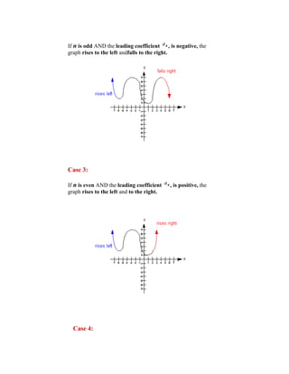
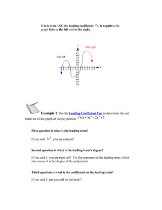
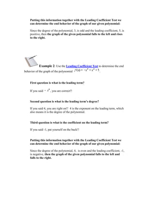
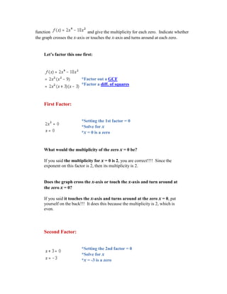
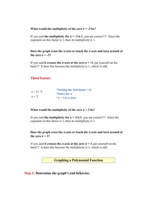
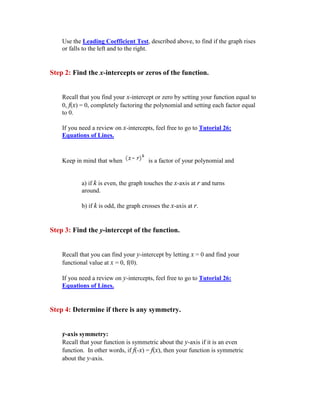
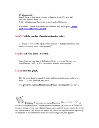
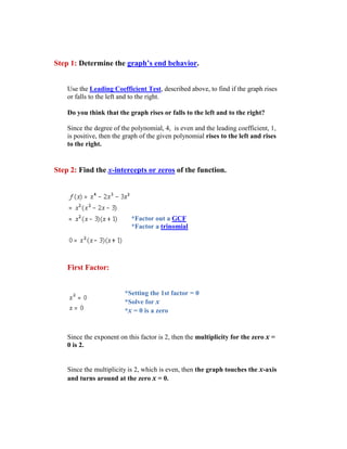
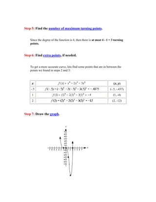
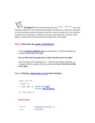
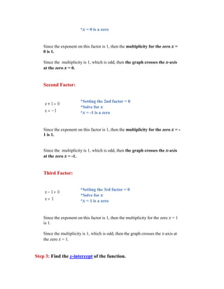
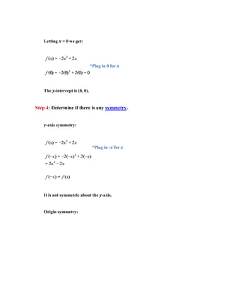
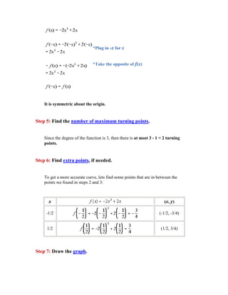
The document discusses graphing polynomial functions. It begins by stating the learning objectives, which include identifying polynomial functions, using the leading coefficient test to determine graph end behavior, finding zeros, determining zero multiplicity, knowing the maximum number of turning points, and graphing polynomial functions. It then provides an introduction and definitions of key polynomial function concepts like leading term, leading coefficient, degree of a term and function, and the leading coefficient test. The document uses examples to demonstrate how to apply the leading coefficient test and find zeros and their multiplicities. It states that a polynomial can have at most n-1 turning points if it has degree n. Finally, it outlines the steps to graph a polynomial function.
The document describes a problem involving combined variation, where the variable z varies jointly as w and x, and inversely as y. It gives the equation of variation as z = kwx/y, where k is the constant of variation. It solves for k when z = 100, w = 4, x = 5, and y = 15, finding that k = 75. Therefore, the equation of combined variation is z = 75wx/y. It then uses this to solve for z when w = 1, x = 5, and y = 3, finding that z = 125.
This document defines and provides examples of arithmetic sequences. An arithmetic sequence is a sequence where each term after the first is obtained by adding a constant value, called the common difference, to the preceding term. The document provides the arithmetic sequence formula and examples of using it to find terms and sums of arithmetic sequences. Various activities are presented for students to practice identifying, describing, and working with arithmetic sequences.
This learner's module discusses about the Six Trigonometric Ratios. It also teaches about the definition and characteristics of each of the Six Trigonometric Ratio.
The document discusses arithmetic and geometric sequences and series. It defines arithmetic and geometric sequences, and provides the formulas for calculating the nth term of each type of sequence. Specifically, it states that the formula for the nth term of an arithmetic sequence is Tn = a + (n-1)d, where a is the first term and d is the common difference. The formula for the nth term of a geometric sequence is Tn = arn-1, where a is the first term and r is the common ratio. The document also provides examples of using these formulas to find terms, common differences or ratios, and to write the formulas for given sequences.
Math 8 - Solving Problems Involving Linear FunctionsCarlo Luna
This document is a mathematics lesson on solving problems involving linear functions. It contains 4 practice problems. Problem 1 has students solve for the number of wallets to be sold to make a Php 30 profit and express the profit function in terms of wallets sold. Problem 2 deals with the cost of manufacturing shoes. Problems 3 has students model the number of math problems Cassandrea solves each day as a linear function and use it to determine how many problems she will solve on specific days. The document concludes by providing an asynchronous learning activity for students to complete.
This module discusses radical expressions and how to simplify them. It covers identifying the radicand and index of radical expressions, simplifying radicals by removing perfect nth roots from the radicand, and rationalizing denominators by removing radicals. The module is designed to teach students to simplify radical expressions, rationalize fractions with radical denominators, and identify radicands and indexes. It provides examples and exercises for students to practice these skills.
Solving Word Problems Involving Quadratic Equationskliegey524
This document provides instructions for solving word problems involving quadratic equations. It explains how to write let statements and equations, solve for consecutive integers or areas, and check solutions. Sample problems are worked through, such as finding two consecutive integers whose sum is 13, or the dimensions of a rectangular garden with an area of 27 square units.
The document discusses solving systems of nonlinear equations in two variables. It provides examples of nonlinear systems that contain equations that are not in the form Ax + By = C, such as x^2 = 2y + 10. Methods for solving nonlinear systems include substitution and addition. The substitution method involves solving one equation for one variable and substituting into the other equation. The addition method involves rewriting the equations and adding them to eliminate variables. Examples demonstrate both methods and finding the solution set that satisfies both equations.
This document provides instructions for using synthetic division to divide polynomials. It contains the following key points:
1. Synthetic division can be used to divide polynomials when the divisor has a leading coefficient of 1 and there is a coefficient for every power of the variable in the numerator.
2. The procedure involves writing the terms of the numerator in descending order, bringing down the constant of the divisor, multiplying and adding down the columns to obtain the coefficients of the quotient polynomial and the remainder.
3. An example problem walks through each step of synthetic division to divide (5x^4 - 4x^2 + x + 6) / (x - 3), obtaining a quotient of 5x^3 + 15
This document provides information about a mathematics instructional material for Grade 9 learners in the Philippines. It was developed collaboratively by educators and reviewed by DepEd. The material covers variations, including direct, inverse, joint, and combined variations. It encourages teachers to provide feedback to DepEd to help improve the material. The material aims to help learners understand different types of variations and solve problems involving variations.
This document discusses arithmetic sequences and their properties. It defines an arithmetic sequence as a sequence where the difference between consecutive terms is constant. It provides the formula for the nth term of an arithmetic sequence as an = a1 + (n-1)d, where a1 is the first term, n is the term number, and d is the common difference. It gives examples of finding specific terms and summarizing sequences. It also discusses the arithmetic mean and arithmetic sum formulas.
This document introduces sequences and series. It defines a sequence as a list of numbers in a specific order, and a series as the sum of the numbers in a sequence. It then discusses two types of sequences: arithmetic and geometric. It provides examples of finite and infinite sequences, and explains how to find partial sums and use summation notation to represent the sum of the first n terms of a sequence.
This document discusses linear functions and how to represent them using equations, graphs, and tables of values. It defines a linear function as one that can be written in the form f(x) = mx + b, where m is the slope and b is the y-intercept. Examples are provided to illustrate determining the slope and y-intercept from an equation and representing a linear function using an equation, table of values, or graph. It is explained that a linear function will produce a straight line on a graph and have constant differences in x- and y-coordinates in its table of values.
1) The document defines algebraic curves as geometric figures formed by the set of points satisfying a given equation relating x and y.
2) Key properties of algebraic curves include their extent (domain and range), symmetry, intercepts, and asymptotes. Symmetry can be tested by substituting -x or -y. Intercepts are where the curve crosses the axes. Asymptotes are lines a curve approaches but never touches.
3) Tracing a curve involves determining its region, testing for symmetry, finding intercepts and asymptotes, and plotting points to sketch the curve.
This document discusses how to graph polynomial functions and find local extrema. It provides instructions on making a table of values, plotting points, connecting them with a smooth curve, and checking end behavior based on the degree and leading coefficient. Extrema are defined as local maxima or minima, where the graph changes from increasing to decreasing. Examples are given to demonstrate graphing polynomials and finding turning points that indicate local extrema.
Grade 10 Math Module 1 searching for patterns, sequence and seriesJocel Sagario
This module introduces sequences and their different types. It discusses finding patterns in sequences to determine the next term. Specific examples are provided to demonstrate writing the first few terms of a sequence given its general formula. The key concepts covered are defining sequences, finite vs infinite sequences, terms of a sequence, increasing vs decreasing sequences, and using the general formula to find specific terms. Students are expected to be able to list terms of sequences, derive the formula, generate terms recursively, and describe arithmetic sequences in different ways.
This document provides a module on linear functions. It defines linear functions as those that can be written in the form f(x) = mx + b, where m is the slope and b is the y-intercept. The module teaches how to determine if a function is linear, rewrite linear equations in slope-intercept form, and graph linear functions given various inputs like two points, x- and y-intercepts, slope and a point, or slope and y-intercept. Examples and practice problems are provided to help students learn to identify, write, and graph different types of linear functions.
The document defines arithmetic sequences and arithmetic means. An arithmetic sequence is a sequence where each term after the first is equal to the preceding term plus a constant value called the common difference. Formulas are provided for calculating any term in the sequence as well as the sum of the first n terms. Arithmetic means refer to the terms between the first and last term of a sequence. Sample problems demonstrate how to find individual terms, sums of terms, and arithmetic means given the first term and common difference of a sequence.
This document discusses how to solve radical equations by isolating the radical expression, removing the radical sign by raising both sides to the appropriate power, and solving the resulting equation. It provides examples of solving various radical equations step-by-step and checking solutions. Key steps include isolating the radical term, removing the radical, solving the resulting equation, and checking for extraneous roots.
This document provides instructions on graphing polynomial functions. It discusses identifying the roots, x-intercepts, and y-intercept from the factored form of the polynomial. It shows working through an example of graphing the function y = (x – 2)(x – 1)(x + 3). The key steps are:
1. Identify the roots and y-intercept
2. Arrange the roots in a table
3. Complete the table by calculating y-values for different x-values
4. Plot the points on a graph
5. Sketch the graph
You will learn how to solve quadratic equations by extracting square roots.
For more instructional resources, CLICK me here! 👇👇👇
https://tinyurl.com/y9muob6q
LIKE and FOLLOW me here! 👍👍👍
https://tinyurl.com/ycjp8r7u
https://tinyurl.com/ybo27k2u
If you are looking for math video tutorials (with voice recording), you may download it on our YouTube Channel. Don't forget to SUBSCRIBE for you to get updated on our upcoming videos.
https://tinyurl.com/y9muob6q
Also, please do visit our page, LIKE and FOLLOW us on Facebook!
https://tinyurl.com/ycjp8r7u
https://tinyurl.com/ybo27k2u
This lesson plan teaches students about inverse functions. It begins with objectives, materials, and a teaching strategy of lecture. Examples are provided to show how to find the inverse of one-to-one functions by interchanging x and y and solving for the new y. Properties are discussed, such as the inverse of an inverse is the original function. Students are asked to find inverses and solve word problems. The lesson concludes by having students generalize their understanding and complete an evaluation with additional inverse problems.
Grade 9: Mathematics Unit 1 Quadratic Equations and Inequalities.Paolo Dagaojes
This document provides an introduction to Module 1 of a mathematics learner's material on quadratic equations and inequalities. It includes 7 objectives that will be covered across 7 lessons. Lesson 1 will illustrate quadratic equations, Lesson 2 will cover solving quadratic equations using extracting square roots, factoring, completing the square, and the quadratic formula. Lesson 3 will discuss the nature of roots of quadratic equations. Lesson 4 will describe the relationship between coefficients and roots. Lesson 5 will solve equations transformable into quadratic equations. Lesson 6 will apply quadratic equations to problems. Lesson 7 will illustrate and solve quadratic inequalities and problems involving them. The document provides the structure and overview of the topics to be discussed in the module.
The document summarizes key characteristics of polynomial functions:
1) Polynomial functions produce smooth, continuous curves on their domains which are the set of real numbers.
2) The graph's x-intercepts, turning points, and absolute/relative maxima and minima are defined.
3) As the degree of a polynomial increases, so do the possible number of x-intercepts and turning points, up to the degree value. The leading coefficient and degree determine whether the graph rises or falls.
This document summarizes key concepts about polynomial functions including:
- Definitions of monomials, polynomials, and polynomial functions
- The standard form and classification of polynomials by degree and number of terms
- How the degree of a polynomial affects the shape of its graph, including the number of turning points and end behavior
- Examples of determining the end behavior and classifying increasing and decreasing parts of polynomial graphs
The document discusses key aspects of polynomials including degree, end behavior, and graph shapes. The degree of a polynomial determines the general shape of its graph and the maximum number of x-intercepts. The end behavior describes what the polynomial function does as it approaches positive and negative infinity, which depends on the sign of the leading term. Polynomials with an even degree and positive leading term have graphs that start and end at positive infinity, while those with an even degree and negative leading term have graphs that start at positive infinity and end at negative infinity.
1. The document discusses writing polynomials in factored form and finding the zeros of polynomial functions. It defines linear factors, roots, zeros, and x-intercepts as equivalent terms.
2. Examples are provided of writing polynomials in factored form using the factor theorem to find the zeros, and then graphing the polynomial function based on its zeros.
3. The factor theorem states that a linear expression x - a is a factor of a polynomial if and only if a is a zero of the related polynomial function. This allows writing a polynomial given its zeros.
This document discusses polynomials, factors, zeros, and graphing polynomial functions. It contains the following key points:
1) A polynomial can be written in factored form by factoring out the greatest common factor and setting each linear factor equal to zero. The zeros of a polynomial function are its x-intercepts.
2) The Factor Theorem states that an expression x - a is a factor of a polynomial if and only if a is a zero of the related polynomial function.
3) To write a polynomial function given its zeros, write each zero as a linear factor and multiply the factors together. Multiple zeros have a linear factor that is repeated, called the multiplicity. The multiplicity indicates if the
This document discusses various methods for estimating and calculating square roots. It begins by defining irrational numbers as non-repeating decimals that can result from taking the square root of a non-perfect square. It then discusses estimating square roots by knowing perfect square numbers and using guess and check methods. Later sections cover using calculators, applying square roots in formulas, exponent rules including multiplication, division, powers, and scientific notation for writing extremely large numbers.
This document discusses polynomial functions including:
1) Identifying polynomials and their degree, evaluating polynomials using synthetic substitution, illustrating polynomial equations, and solving problems involving polynomials.
2) Defining a polynomial function as a function involving only positive integer exponents of a variable and noting the highest power as its degree, with the domain being all real numbers.
3) Providing examples of types of polynomial functions and graphs of polynomial functions, and evaluating polynomials using direct substitution or synthetic substitution.
This document provides an overview of linear equations in one variable. It defines a linear equation as one that can be written in the form ax = b, where a and b are real numbers and a ≠ 0. Parts of a linear equation like the variable, coefficient, constants, and left and right hand sides are explained. It also discusses how to solve linear equations by finding the value of the variable that makes the left and right sides equal. Several examples are provided of how to translate word problems into linear equations and solve them. Real-world applications of linear equations discussed include comparing rates of pay from different jobs and calculating cab fares.
This document provides information about functions and relations in mathematics. It contains the following:
1) A definition of a relation as a set of related information with two types of data that can be graphed on a coordinate plane.
2) An explanation that functions are "well-behaved" relations where each x-value relates to only one y-value.
3) An example of a relation that is a function because each number in the x column corresponds to only one number in the y column.
The document defines terms related to polynomials such as numerical coefficient, literal coefficient, degree, similar terms, monomial, binomial, trinomial, multinomial. It also defines the different kinds of polynomials according to the number of terms and degree such as constant, linear, quadratic, cubic, quartic, quintic polynomials. It provides examples of determining the degree, kind according to number of terms, leading term, leading coefficient of a polynomial and writing it in standard form.
This document discusses evaluating and graphing polynomial functions. It defines a polynomial as a function with positive integer exponents. It explains that polynomials have a leading coefficient, constant term, and degree. Linear functions have a degree of 1, and quadratic functions have a degree of 2. The document provides instructions for writing polynomials in standard form and discusses using tables of values and analyzing end behavior to graph polynomials.
Logarithms relate an input value to the power needed to raise a base to produce that output value. Logarithmic scales are used to measure sound because they match how humans perceive changes in loudness. The key properties of logarithms are:
1) Logarithmic functions are inverses of exponential functions.
2) When working with logarithms or exponents, it helps to rewrite the problem in the other form.
3) For logarithmic equations, setting the arguments equal is valid if the bases are the same.
Logarithms relate an input value to the power needed to raise a base to produce that output value. Logarithmic scales are used to measure sound because they allow for large ranges of intensity to be represented on a linear scale. The key properties of logarithms are:
1) Logarithmic functions are inverses of exponential functions.
2) When working with logarithms or exponentials, it helps to rewrite the problem in the other form.
3) For logarithmic equations, setting the arguments equal is valid if the bases are the same.
The document provides information about linear and nonlinear expressions including:
- Definitions of linear and nonlinear expressions, where linear expressions can only have x terms with an exponent of 1 and nonlinear expressions have exponents not equal to 1 or 0.
- Examples of sorting expressions into linear and nonlinear groups and explaining the reasoning. Linear expressions follow the definition while nonlinear have exponents not 1 or 0.
- The importance of distinguishing between linear and nonlinear expressions is because students will soon learn to solve linear equations, with nonlinear equations addressed later. It also relates to predicting graph shapes.
- Additional examples analyze expressions and identify them as linear or nonlinear based on the definitions and exponents of x terms. Students are instructed to practice identifying expressions
Students will be taking standardized tests from October 26th to 30th so there will be no live classes during that time. The document provides definitions and examples to help students distinguish between linear and nonlinear expressions. Linear expressions can only have variables raised to the power of 1 or 0, while nonlinear expressions have variables raised to other powers. Being able to identify linear and nonlinear expressions is important because students will be learning to solve linear equations, and want to predict the shapes of their graphs. A series of examples are provided to help students apply the definitions.
Advanced functions ppt (Chapter 1) part iiTan Yuhang
This document provides definitions and examples to explain how to graph polynomial functions. It discusses determining the degree of the polynomial, the sign of the leading coefficient, end behavior, x- and y-intercepts, and intervals of increase and decrease. Examples are provided to demonstrate how to find zeros, or x-intercepts, and their multiplicities in order to properly graph the polynomial based on these features.
This document discusses key concepts for graphing polynomial functions including:
1. The degree of the polynomial determines the end behavior and maximum number of turns.
2. The sign of the leading coefficient indicates whether the graph faces up or down on both ends.
3. X-intercepts and y-intercepts are found by setting the polynomial equal to 0 or the variable equal to 0.
4. The multiplicity of intercepts determines whether the graph crosses or touches the x-axis at that point.
This document discusses mathematical language and symbols. It defines a variable as a placeholder that can represent unknown values or elements in a set. Variables allow statements to be generalized rather than restricted to specific values. Different types of mathematical statements are described, including universal statements that are true for all cases, conditional statements with an "if-then" structure, and existential statements that assert the existence of something satisfying a property. Universal conditional and universal existential statements are explained as combining characteristics of different statement types. Examples are provided to illustrate rewriting sentences using variables and different types of mathematical statements.
Requirements.docxRequirementsFont Times New RomanI NEED .docxheunice
Requirements.docx
Requirements:
Font: Times New Roman
I NEED 7 APA Style reference and In-text citation
Spacing: SINGLE
All the number of words are included next to the questions.
__________________________________________________________________________________
BSBLDR511 - Develop and use emotional intelligence
Questions:
1. Explain emotional intelligence principles and strategies (100 words)
2. Describe the relationship between emotionally effective people and the attainment of business objectives (100 words)
3. Explain how to communicate with a diverse workforce which has varying cultural expressions of emotion (100 words)
4. List at least five (5) examples of emotional strengths and weaknesses. Explain all. (100 words)
5. Identify at least three (3) examples of emotional states you might identify in co-workers in the workplace, and outline the common cues for each. (100 words)
6. Why is it essential to consider varying cultural expressions of emotions when working and responding to emotional cues in a diverse workforce? (100 words)
7. There are a variety of opportunities you may provide in your workplace for others to express their thoughts and feelings. List two (2). ( 100 words)
8. Why is it important to assist others to understand the effect of their behavior and emotions on others in the workplace? ( 100 words)
9. What information will you need to consider to ensure you use the strengths of workgroup members to achieve workplace outcomes? (100 words)
Quiz 8 Notes
Scatterplots, Correlation and Regression
We are turning to our last quiz topic; regression. To get to regression, we need to understand several concepts first.
To start with, we will be working with two quantitative variables. The goal is to see if there is a relationship/association between the two variables. As one variable increases, what does the second variable do? If the second variable makes a consistent change then a relationship may exist. MAJOR POINT: saying a relationship exists does NOT mean there is Causation. The greatest abuse of statistical work is here, when a person runs a regression then says Variable A causes Variable B to change. You must have experimental results to establish causation.
Looking at the two variables that will be in a regression you need to know that each variable plays a specific role. One of the variables, X, will be the independent/explanatory variable and the other, Y, will be the dependent/ response variable. In a regression we are looking to see if changes in, Y; occur as X changes. It is very important that you establish at the beginning which of your variables will be X and which will be Y. Swapping the places for the two variables may not work. Let’s do an example.
In economics, we discuss the relationship of the quantity demand and the price of a good. Which one would be the X in a regression, and which would be, Y? The Law of Demand says, “as the price of a good increases, the quantity demanded decreases”. Which is allow.
This document provides an overview of key concepts related to graphing polynomials, including:
1. Definitions of terms like intervals of increase/decrease, odd/even functions, zeros, and multiplicities.
2. Steps for graphing polynomials which include determining behavior, finding intercepts and zeros, and joining points based on multiplicities.
3. Examples are provided to demonstrate finding zeros and their multiplicities, and graphing a polynomial based on the identified features.
4. Information that can be determined from a polynomial graph, such as degree, leading coefficient, end behavior, intercepts, and intervals of increase/decrease.
Nigeria has a varied landscape ranging from tropical rainforest in the south to savannah in the center and the Sahara Desert in the far north. It has over 200 million people and 36 states. The major environmental issues include oil pollution in the Niger Delta, waste management problems in major cities, and risks from climate change like reduced food production. Nigeria's educational system has three levels - basic, post-basic, and tertiary education. It is the shared responsibility of federal, state and local governments and includes public and private institutions.
The document summarizes Finland's educational system from pre-primary education through adult education. It outlines that basic education is compulsory and free for all students between the ages of 7-16 provided at comprehensive schools. Vocational education and training provides qualifications and degrees in fields like technology, health, and business. Polytechnics and universities provide professional degrees and conduct research. Adult education programs are available in vocational schools, polytechnics, universities, and liberal adult education centers to support lifelong learning and professional development. Financial assistance is available to students in the form of grants, housing supplements, and government-backed loans.
Egypt is located in northern Africa, bordered by Libya, the Gaza Strip, Sudan, and the Mediterranean Sea. Arabic is the official language, while English and French are widely understood. Education is state-sponsored and divided into primary, preparatory, secondary, and higher education. Female education has increased over the years, with girls outperforming boys and occupying top ranks. While the number of females in science and engineering fields has risen, cultural stereotypes still influence some to pursue other fields. Overall, Egypt aims to continue improving access to education and educational quality.
Venezuela is a country located on the northern coast of South America with a population of approximately 29 million people. The majority of Venezuelans are Roman Catholic but Evangelical Protestants make up about 10% of the population. Venezuela's population is ethnically diverse, with most identifying as multiracial or white. The official currency is the bolívar fuerte which replaced the bolívar in 2008 due to inflation. While Spanish is the dominant language, indigenous languages like Wayuu and Warao are also recognized. Venezuela has a unicameral legislature and a president who is both head of state and government, elected to a six-year term by popular vote. Education is compulsory for nine years in Venezuela and
Each teacher is provided with a Korean assistant who helps with translation,
cultural issues, paperwork and other daily tasks. This assistant is usually a student or
recent graduate who speaks excellent English.
Vacation Time: Teachers receive paid national holidays and summer/winter breaks.
National holidays include New Years, Lunar New Year, Independence Movement Day
and more. Summer break is usually 6 weeks and winter break is 2 weeks.
Health Insurance: All teachers receive national health insurance which covers the cost
of doctor visits and hospital stays. Some schools also provide additional private
insurance.
Severance Pay: Upon completion of the contract, teachers receive a lump sum
severance payment equal to one month's salary for
Malaysia is located in Southeast Asia and consists of two parts - peninsular Malaysia and east Malaysia. The official language is Bahasa Malaysia and the dominant religion is Islam. During British rule, there were vernacular schools that used different languages but did not foster national unity. After World War 2, committees were formed to develop a national education system using a common syllabus and examinations to unite the multiethnic population through the use of Malay and English as compulsory subjects. This led to the Education Act of 1961 that established the foundation of Malaysia's current education system.
Education in Libya has evolved significantly over time. During Ottoman rule in the 16th-20th centuries, small Koran schools were the primary form of education. Italy expanded the school system when it controlled Libya but excluded Arabs and Bedouins. After independence, Libya built new schools and universities while also reopening Koran schools, and enrollment increased rapidly. However, Libya still struggles with shortages of qualified teachers and low attendance among females in secondary and higher education.
Implementing rules and regulations of k to 12Allan Gulinao
This document provides the implementing rules and regulations for the Enhanced Basic Education Act of 2013. It defines key terms, outlines the scope of basic education which now includes kindergarten and 12 years of elementary and secondary education. It also discusses provisions for developing an inclusive curriculum that follows standards like being learner-centered and using the mother tongue as the primary language of instruction, especially in early grades of elementary school. The rules aim to strengthen and expand basic education in the Philippines as mandated by the new law.
Canada is the second largest country in the world located in North America. It has ten provinces and three territories, with six time zones across the vast country. Ottawa is the capital city located in Ontario. Canada has a diverse population of over 34 million people from many different cultures and nationalities. It has a highly developed economy and ranks highly for quality of living. Some of Canada's major cities include Vancouver, Toronto, Calgary, Montreal, and Edmonton.
This lesson plan aims to teach students about angles formed by parallel lines cut by a transversal. It begins with introducing the objectives of defining a transversal and identifying different angles formed. The instructional procedure includes reviewing perpendicular lines, presenting examples and activities, and having students apply their learning by identifying angles in figures. For evaluation, students are asked to identify exterior, interior, alternate interior, and alternate exterior angles. The lesson concludes with an assignment for students to classify different angles in a figure using a transversal.
The key principles of Finnish education policy are quality, efficiency, equity and internationalization. Education is free at all levels from pre-primary to higher education. The education system consists of pre-primary education, nine years of compulsory basic education, upper secondary education and higher education. Education policy priorities are outlined in five-year development plans which currently focus on promoting equality, quality and lifelong learning. Legislation governs each level of education and most education is publicly funded through state and local authorities. Evaluation of education focuses on both self-evaluation of schools and national evaluations.
A lesson plan guides classroom instruction by detailing the objectives, activities, and assessments for a lesson. It helps teachers stay organized, engage students, and ensure all required topics are covered. While developing detailed lesson plans requires time, it saves effort in the long run and improves teaching skills. Lesson plans provide structure for students and allow teachers to efficiently manage their time and resources.
বাংলাদেশের অর্থনৈতিক সমীক্ষা ২০২৪ [Bangladesh Economic Review 2024 Bangla.pdf] কম্পিউটার , ট্যাব ও স্মার্ট ফোন ভার্সন সহ সম্পূর্ণ বাংলা ই-বুক বা pdf বই " সুচিপত্র ...বুকমার্ক মেনু 🔖 ও হাইপার লিংক মেনু 📝👆 যুক্ত ..
আমাদের সবার জন্য খুব খুব গুরুত্বপূর্ণ একটি বই ..বিসিএস, ব্যাংক, ইউনিভার্সিটি ভর্তি ও যে কোন প্রতিযোগিতা মূলক পরীক্ষার জন্য এর খুব ইম্পরট্যান্ট একটি বিষয় ...তাছাড়া বাংলাদেশের সাম্প্রতিক যে কোন ডাটা বা তথ্য এই বইতে পাবেন ...
তাই একজন নাগরিক হিসাবে এই তথ্য গুলো আপনার জানা প্রয়োজন ...।
বিসিএস ও ব্যাংক এর লিখিত পরীক্ষা ...+এছাড়া মাধ্যমিক ও উচ্চমাধ্যমিকের স্টুডেন্টদের জন্য অনেক কাজে আসবে ...
A Strategic Approach: GenAI in EducationPeter Windle
Artificial Intelligence (AI) technologies such as Generative AI, Image Generators and Large Language Models have had a dramatic impact on teaching, learning and assessment over the past 18 months. The most immediate threat AI posed was to Academic Integrity with Higher Education Institutes (HEIs) focusing their efforts on combating the use of GenAI in assessment. Guidelines were developed for staff and students, policies put in place too. Innovative educators have forged paths in the use of Generative AI for teaching, learning and assessments leading to pockets of transformation springing up across HEIs, often with little or no top-down guidance, support or direction.
This Gasta posits a strategic approach to integrating AI into HEIs to prepare staff, students and the curriculum for an evolving world and workplace. We will highlight the advantages of working with these technologies beyond the realm of teaching, learning and assessment by considering prompt engineering skills, industry impact, curriculum changes, and the need for staff upskilling. In contrast, not engaging strategically with Generative AI poses risks, including falling behind peers, missed opportunities and failing to ensure our graduates remain employable. The rapid evolution of AI technologies necessitates a proactive and strategic approach if we are to remain relevant.
How to Add Chatter in the odoo 17 ERP ModuleCeline George
In Odoo, the chatter is like a chat tool that helps you work together on records. You can leave notes and track things, making it easier to talk with your team and partners. Inside chatter, all communication history, activity, and changes will be displayed.
Introduction to AI for Nonprofits with Tapp NetworkTechSoup
Dive into the world of AI! Experts Jon Hill and Tareq Monaur will guide you through AI's role in enhancing nonprofit websites and basic marketing strategies, making it easy to understand and apply.
How to Manage Your Lost Opportunities in Odoo 17 CRMCeline George
Odoo 17 CRM allows us to track why we lose sales opportunities with "Lost Reasons." This helps analyze our sales process and identify areas for improvement. Here's how to configure lost reasons in Odoo 17 CRM
This slide is special for master students (MIBS & MIFB) in UUM. Also useful for readers who are interested in the topic of contemporary Islamic banking.
A workshop hosted by the South African Journal of Science aimed at postgraduate students and early career researchers with little or no experience in writing and publishing journal articles.
This presentation was provided by Steph Pollock of The American Psychological Association’s Journals Program, and Damita Snow, of The American Society of Civil Engineers (ASCE), for the initial session of NISO's 2024 Training Series "DEIA in the Scholarly Landscape." Session One: 'Setting Expectations: a DEIA Primer,' was held June 6, 2024.
June 3, 2024 Anti-Semitism Letter Sent to MIT President Kornbluth and MIT Cor...Levi Shapiro
Letter from the Congress of the United States regarding Anti-Semitism sent June 3rd to MIT President Sally Kornbluth, MIT Corp Chair, Mark Gorenberg
Dear Dr. Kornbluth and Mr. Gorenberg,
The US House of Representatives is deeply concerned by ongoing and pervasive acts of antisemitic
harassment and intimidation at the Massachusetts Institute of Technology (MIT). Failing to act decisively to ensure a safe learning environment for all students would be a grave dereliction of your responsibilities as President of MIT and Chair of the MIT Corporation.
This Congress will not stand idly by and allow an environment hostile to Jewish students to persist. The House believes that your institution is in violation of Title VI of the Civil Rights Act, and the inability or
unwillingness to rectify this violation through action requires accountability.
Postsecondary education is a unique opportunity for students to learn and have their ideas and beliefs challenged. However, universities receiving hundreds of millions of federal funds annually have denied
students that opportunity and have been hijacked to become venues for the promotion of terrorism, antisemitic harassment and intimidation, unlawful encampments, and in some cases, assaults and riots.
The House of Representatives will not countenance the use of federal funds to indoctrinate students into hateful, antisemitic, anti-American supporters of terrorism. Investigations into campus antisemitism by the Committee on Education and the Workforce and the Committee on Ways and Means have been expanded into a Congress-wide probe across all relevant jurisdictions to address this national crisis. The undersigned Committees will conduct oversight into the use of federal funds at MIT and its learning environment under authorities granted to each Committee.
• The Committee on Education and the Workforce has been investigating your institution since December 7, 2023. The Committee has broad jurisdiction over postsecondary education, including its compliance with Title VI of the Civil Rights Act, campus safety concerns over disruptions to the learning environment, and the awarding of federal student aid under the Higher Education Act.
• The Committee on Oversight and Accountability is investigating the sources of funding and other support flowing to groups espousing pro-Hamas propaganda and engaged in antisemitic harassment and intimidation of students. The Committee on Oversight and Accountability is the principal oversight committee of the US House of Representatives and has broad authority to investigate “any matter” at “any time” under House Rule X.
• The Committee on Ways and Means has been investigating several universities since November 15, 2023, when the Committee held a hearing entitled From Ivory Towers to Dark Corners: Investigating the Nexus Between Antisemitism, Tax-Exempt Universities, and Terror Financing. The Committee followed the hearing with letters to those institutions on January 10, 202
Executive Directors Chat Leveraging AI for Diversity, Equity, and InclusionTechSoup
Let’s explore the intersection of technology and equity in the final session of our DEI series. Discover how AI tools, like ChatGPT, can be used to support and enhance your nonprofit's DEI initiatives. Participants will gain insights into practical AI applications and get tips for leveraging technology to advance their DEI goals.
Strategies for Effective Upskilling is a presentation by Chinwendu Peace in a Your Skill Boost Masterclass organisation by the Excellence Foundation for South Sudan on 08th and 09th June 2024 from 1 PM to 3 PM on each day.
Your Skill Boost Masterclass: Strategies for Effective Upskilling
Graph of polynomial function
1. Learning Objectives
After completing this tutorial, you should be able to:
1. Identify a polynomial function.
2. Use the Leading Coefficient Test to find the end behavior of the graph
of a given polynomial function.
3. Find the zeros of a polynomial function.
4. Find the multiplicity of a zero and know if the graph crosses the x-axis
at the zero or touches the x-axis and turns around at the zero.
5. Know the maximum number of turning points a graph of a polynomial
function could have.
6. Graph a polynomial function.
Introduction
In this tutorial we will be looking at graphs of polynomial functions. If you need a
review on functions, feel free to go to Tutorial 30: Introduction to Functions. If you
need a review on polynomials in general, feel free to go to Tutorial 6: Polynomials.
Basically, the graph of a polynomial function is a smooth continuous curve. There are
several main aspects of this type of graph that you can use to help put the curve
together. I will be going over how to use the leading term of your polynomial function
to determine the end behavior of its graph. We will also be looking at finding the
zeros, aka the x-intercepts, as well as the y-intercept of the graph. If you need a review
on intercepts, feel free to go to Tutorial 26: Equations of Lines. Another important
concept is to know the largest possible number of turning points. This will help you
be more accurate in the graph that you draw. That just about covers it. I guess you are
ready to get to it.
2. Tutorial
Polynomial Function
A polynomial function is a function that can be written
in the form
, where
are real numbers and
n is a nonnegative integer.
Basically it is a function whose rule is given by a polynomial in one variable.
If you need a review on functions, feel free to go to Tutorial 30: Introduction to
Functions. If you need a review on polynomials in general, feel free to go to Tutorial
6: Polynomials.
An example of a polynomial function is .
Leading Term
When the polynomial function is written in standard
form,
,
the leading term is .
3. In other words, the leading term is the term that the variable has its highest exponent.
The leading term of the function would be .
Leading Coefficient
When the polynomial function is written in standard
form,
,
the leading coefficient is .
Basically, the leading coefficient is the coefficient on the leading term.
The leading coefficient of the function would be - 4.
Degree of a Term of a Polynomial Function
The degree of a term of a polynomial function is the exponent on the variable.
Degree of a Polynomial Function
When the polynomial function is written in standard
form,
4. ,
the degree of the polynomial function is n.
The degree of the polynomial is the largest degree of all of its terms.
The degree of the function would be 7.
The Leading Coefficient Test
There are four cases that go with this test:
Given a polynomial function in standard
form :
Case 1:
If n is odd AND the leading coefficient , is positive, the
graph falls to the left andrises to the right:
Case 2:
5. If n is odd AND the leading coefficient , is negative, the
graph rises to the left andfalls to the right.
Case 3:
If n is even AND the leading coefficient , is positive, the
graph rises to the left and to the right.
Case 4:
6. If n is even AND the leading coefficient , is negative, the
graph falls to the left and to the right.
Example 1: Use the Leading Coefficient Test to determine the end
behavior of the graph of the polynomial .
First question is what is the leading term?
If you said , you are correct!!
Second question is what is the leading term’s degree?
If you said 3, you are right on!! 3 is the exponent on the leading term, which
also means it is the degree of the polynomial.
Third question is what is the coefficient on the leading term?
If you said 5, pat yourself on the back!!
7. Putting this information together with the Leading Coefficient Test we
can determine the end behavior of the graph of our given polynomial:
Since the degree of the polynomial, 3, is odd and the leading coefficient, 5, is
positive, then the graph of the given polynomial falls to the left and rises
to the right.
Example 2: Use the Leading Coefficient Test to determine the end
behavior of the graph of the polynomial .
First question is what is the leading term?
If you said , you are correct!!
Second question is what is the leading term’s degree?
If you said 4, you are right on!! 4 is the exponent on the leading term, which
also means it is the degree of the polynomial.
Third question is what is the coefficient on the leading term?
If you said -1, pat yourself on the back!!
Putting this information together with the Leading Coefficient Test we
can determine the end behavior of the graph of our given polynomial:
Since the degree of the polynomial, 4, is even and the leading coefficient, -1,
is negative, then the graph of the given polynomial falls to the left and
falls to the right.
8. Example 3: Use the Leading Coefficient Test to determine the end
behavior of the graph of the polynomial .
First question is what is the leading term?
If you said , you are correct!!
Second question is what is the leading term’s degree?
If you said 5, you are right on!! 5 is the exponent on the leading term, which
also means it is the degree of the polynomial.
Third question is what is the coefficient on the leading term?
If you said -7, pat yourself on the back!!
Putting this information together with the Leading Coefficient Test we
can determine the end behavior of the graph of our given polynomial:
Since the degree of the polynomial, 5, is odd and the leading coefficient, -7,
is negative, then the graph of the given polynomial rises to the left and
falls to the right.
Example 4: Use the Leading Coefficient Test to determine the end
behavior of the graph of the polynomial .
First question is what is the leading term?
If you said , you are correct!!
9. Second question is what is the leading term’s degree?
If you said 6, you are right on!! 6 is the exponent on the leading term, which
also means it is the degree of the polynomial.
Third question is what is the coefficient on the leading term?
If you said 1, pat yourself on the back!!
Putting this information together with the Leading Coefficient Test we
can determine the end behavior of the graph of our given polynomial:
Since the degree of the polynomial, 6, is even and the leading coefficient, 1,
is positive, then the graph of the given polynomial rises to the left and
rises to the right.
Zeros (or Roots) of Polynomial Functions
A zero or root of a polynomial function is the value of x such that f(x) =
0.
In other words it is the x-intercept, where the functional value or y is equal to
0.
Zero of Multiplicity k
If is a factor of a polynomial
function f and
is not a factor of f, then r is called a
10. zero of
multiplicity k of f.
In other words, when a polynomial function is set equal to zero and has been
completely factored and each different factor is written with the highest
appropriate exponent, depending on the number of times that factor occurs in
the product, the exponent on the factor that the zero is a solution for, gives
the multiplicity of that zero.
The exponent indicates how many times that factor would be written out in
the product, this gives us a multiplicity.
Multiplicity of Zeros and the x-intercept
There are two cases that go with this concept:
Case 1:
If r is a zero of even multiplicity:
This means the graph touches the x-axis at r and turns around.
This happens because the sign of f(x) does not change from
one side to the other side of r.
Case 2:
If r is a zero of odd multiplicity:
This means the graph crosses the x-axis at r.
This happens because the sign of f(x) changes from one side
to the other side of r.
11. Turning Points
If f is a polynomial function of degree n, then
there is at most n - 1 turning points on the graph of f.
A turning point is a point at which the graph changes direction.
Keep in mind that you can have fewer than n - 1 turning points, but it will never
exceed n - 1 turning points.
Example 5: Find the zeros for the polynomial
function and give the multiplicity for each zero. Indicate
whether the graph crosses the x-axis or touches the x-axis and turns around at each
zero.
First Factor:
The first factor is 3, which is a constant. Therefore, there are no zeros that go
with this factor.
Second Factor:
*Setting the 2nd factor = 0
*Solve for x
*x = -1/2 is a zero
12. What would the multiplicity of the zero x = -1/2 be?
If you said the multiplicity for x = -1/2 is 4, you are correct!!!! Since the
exponent on this factor is 4, then its multiplicity is 4.
Does the graph cross the x-axis or touch the x-axis and turn around at
the zero x = -1/2?
If you said it touches the x-axis and turns around at the zero x = -1/2, pat
yourself on the back!!! It does this because the multiplicity is 4, which is
even.
Third Factor:
*Setting the 3rd factor = 0
*Solve for x
*x = 4 is a zero
What would the multiplicity of the zero x = 4 be?
If you said the multiplicity for x = 4 is 3, you are correct!!!! Since the
exponent on this factor is 3, then its multiplicity is 3.
Does the graph cross the x-axis or touch the x-axis and turn around at
the zero x = 4?
If you said it crosses the x-axis at the zero x = 4, pat yourself on the
back!!! It does this because the multiplicity is 3, which is odd.
Example 6: Find the zeros for the polynomial
13. function and give the multiplicity for each zero. Indicate whether
the graph crosses the x-axis or touches the x-axis and turns around at each zero.
Let’s factor this one first:
*Factor out a GCF
*Factor a diff. of squares
First Factor:
*Setting the 1st factor = 0
*Solve for x
*x = 0 is a zero
What would the multiplicity of the zero x = 0 be?
If you said the multiplicity for x = 0 is 2, you are correct!!!! Since the
exponent on this factor is 2, then its multiplicity is 2.
Does the graph cross the x-axis or touch the x-axis and turn around at
the zero x = 0?
If you said it touches the x-axis and turns around at the zero x = 0, pat
yourself on the back!!! It does this because the multiplicity is 2, which is
even.
Second Factor:
*Setting the 2nd factor = 0
*Solve for x
*x = -3 is a zero
14. What would the multiplicity of the zero x = -3 be?
If you said the multiplicity for x = -3 is 1, you are correct!!!! Since the
exponent on this factor is 1, then its multiplicity is 1.
Does the graph cross the x-axis or touch the x-axis and turn around at
the zero x = -3?
If you said it crosses the x-axis at the zero x = -3, pat yourself on the
back!!! It does this because the multiplicity is 1, which is odd.
Third Factor:
*Setting the 3rd factor = 0
*Solve for x
*x = 3 is a zero
What would the multiplicity of the zero x = 3 be?
If you said the multiplicity for x = 3 is 1, you are correct!!!! Since the
exponent on this factor is 1, then its multiplicity is 1.
Does the graph cross the x-axis or touch the x-axis and turn around at
the zero x = 3?
If you said it crosses the x-axis at the zero x = 3, pat yourself on the
back!!! It does this because the multiplicity is 1, which is odd.
Graphing a Polynomial Function
Step 1: Determine the graph’s end behavior.
15. Use the Leading Coefficient Test, described above, to find if the graph rises
or falls to the left and to the right.
Step 2: Find the x-intercepts or zeros of the function.
Recall that you find your x-intercept or zero by setting your function equal to
0, f(x) = 0, completely factoring the polynomial and setting each factor equal
to 0.
If you need a review on x-intercepts, feel free to go to Tutorial 26:
Equations of Lines.
Keep in mind that when is a factor of your polynomial and
a) if k is even, the graph touches the x-axis at r and turns
around.
b) if k is odd, the graph crosses the x-axis at r.
Step 3: Find the y-intercept of the function.
Recall that you can find your y-intercept by letting x = 0 and find your
functional value at x = 0, f(0).
If you need a review on y-intercepts, feel free to go to Tutorial 26:
Equations of Lines.
Step 4: Determine if there is any symmetry.
y-axis symmetry:
Recall that your function is symmetric about the y-axis if it is an even
function. In other words, if f(-x) = f(x), then your function is symmetric
about the y-axis.
16. Origin symmetry:
Recall that your function is symmetric about the origin if it is an odd
function. In other words, if
f(-x) = -f(x), then your function is symmetric about the origin.
If you need a review on even and odd functions, feel free to go to Tutorial
32: Graphs of Functions, Part II.
Step 5: Find the number of maximum turning points.
As discussed above, if f is a polynomial function of degree n, then there is at
most n - 1 turning points on the graph off.
Step 6: Find extra points, if needed.
Sometimes you may need to find points that are in between the ones you
found in steps 2 and 3 to help you be more accurate on your graph.
Step 7: Draw the graph.
Plot the points found in steps 2, 3, and 6 and use the information gathered in
steps 1, 2, 4, and 5 to draw your graph.
The graph of polynomial functions is always a smooth continuous curve.
Example 7: Given the polynomial function a)
use the Leading Coefficient Test to determine the graph’s end behavior, b) find the x-
intercepts (or zeros) and state whether the graph crosses the x-axis or touches the x-axis
and turns around at each x-intercept, c) find the y-intercept, d) determine the symmetry
of the graph, e) indicate the maximum possible turning points, and f) graph.
17. Step 1: Determine the graph’s end behavior.
Use the Leading Coefficient Test, described above, to find if the graph rises
or falls to the left and to the right.
Do you think that the graph rises or falls to the left and to the right?
Since the degree of the polynomial, 4, is even and the leading coefficient, 1,
is positive, then the graph of the given polynomial rises to the left and rises
to the right.
Step 2: Find the x-intercepts or zeros of the function.
*Factor out a GCF
*Factor a trinomial
First Factor:
*Setting the 1st factor = 0
*Solve for x
*x = 0 is a zero
Since the exponent on this factor is 2, then the multiplicity for the zero x =
0 is 2.
Since the multiplicity is 2, which is even, then the graph touches the x-axis
and turns around at the zero x = 0.
18. Second Factor:
*Setting the 2nd factor = 0
*Solve for x
*x = 3 is a zero
Since the exponent on this factor is 1, then the multiplicity for the zero x =
3 is 1.
Since the multiplicity is 1, which is odd, then the graph crosses the x-axis
at the zero x = 3.
Third Factor:
*Setting the 3rd factor = 0
*Solve for x
*x = -1 is a zero
Since the exponent on this factor is 1, then the multiplicity for the zero x = -1
is 1.
Since the multiplicity is 1, which is odd, then the graph crosses the x-axis at
the zero x = -1.
Step 3: Find the y-intercept of the function.
Letting x = 0 we get:
*Plug in 0 for x
19. The y-intercept is (0, 0).
Step 4: Determine if there is any symmetry.
y-axis symmetry:
*Plug in -x for x
It is not symmetric about the y-axis.
Origin symmetry:
*Plug in -x for x
*Take the opposite of f(x)
It is not symmetric about the origin.
20. Step 5: Find the number of maximum turning points.
Since the degree of the function is 4, then there is at most 4 - 1 = 3 turning
points.
Step 6: Find extra points, if needed.
To get a more accurate curve, lets find some points that are in between the
points we found in steps 2 and 3:
x (x, y)
-.5 (-.5, -.437)
1 (1, -4)
2 (2, -12)
Step 7: Draw the graph.
21. Example 8: Given the polynomial function a) use the
Leading Coefficient Test to determine the graph’s end behavior, b) find the x-intercepts
(or zeros) and state whether the graph crosses the x-axis or touches the x-axis and turns
around at each x-intercept, c) find the y-intercept, d) determine the symmetry of the
graph, e) indicate the maximum possible turning points, and f) graph.
Step 1: Determine the graph’s end behavior.
Use the Leading Coefficient Test, described above, to find if the graph rises
or falls to the left and to the right.
Do you think that the graph rises or falls to the left and to the right?
Since the degree of the polynomial, 3, is odd and the leading coefficient, -2,
is negative, then the graph of the given polynomial rises to the left and falls
to the right.
Step 2: Find the x-intercepts or zeros of the function.
*Factor out a GCF
*Factor a diff. of squares
First Factor:
*Setting the 1st factor = 0
*Solve for x
22. *x = 0 is a zero
Since the exponent on this factor is 1, then the multiplicity for the zero x =
0 is 1.
Since the multiplicity is 1, which is odd, then the graph crosses the x-axis
at the zero x = 0.
Second Factor:
*Setting the 2nd factor = 0
*Solve for x
*x = -1 is a zero
Since the exponent on this factor is 1, then the multiplicity for the zero x = -
1 is 1.
Since the multiplicity is 1, which is odd, then the graph crosses the x-axis
at the zero x = -1.
Third Factor:
*Setting the 3rd factor = 0
*Solve for x
*x = 1 is a zero
Since the exponent on this factor is 1, then the multiplicity for the zero x = 1
is 1.
Since the multiplicity is 1, which is odd, then the graph crosses the x-axis at
the zero x = 1.
Step 3: Find the y-intercept of the function.
23. Letting x = 0 we get:
*Plug in 0 for x
The y-intercept is (0, 0).
Step 4: Determine if there is any symmetry.
y-axis symmetry:
*Plug in -x for x
It is not symmetric about the y-axis.
Origin symmetry:
24. *Plug in -x for x
*Take the opposite of f(x)
It is symmetric about the origin.
Step 5: Find the number of maximum turning points.
Since the degree of the function is 3, then there is at most 3 - 1 = 2 turning
points.
Step 6: Find extra points, if needed.
To get a more accurate curve, lets find some points that are in between the
points we found in steps 2 and 3:
x (x, y)
-1/2 (-1/2, -3/4)
1/2 (1/2, 3/4)
Step 7: Draw the graph.
25. Practice Problems
These are practice problems to help bring you to the next level. It will allow you to
check and see if you have an understanding of these types of problems. Math works
just like anything else, if you want to get good at it, then you need to practice it.
Even the best athletes and musicians had help along the way and lots of practice,
practice, practice, to get good at their sport or instrument. In fact there is no such
thing as too much practice.
To get the most out of these, you should work the problem out on your own and
then check your answer by clicking on the link for the answer/discussion for that
problem. At the link you will find the answer as well as any steps that went into
finding that answer.
Practice Problems 1a - 1b: Given the polynomial function a) use the
Leading Coefficient Test to determine the graph’s end behavior, b) find the x-
intercepts (or zeros) and state whether the graph crosses the x-axis or touches
the x-axis and turns around at each x-intercept, c) find the y-intercept, d)
26. determine the symmetry of the graph, e) indicate the maximum possible turning
points, and f) graph.
1a.
1b.
(answer/discussion to 1b)
(answer/discussion to 1a)