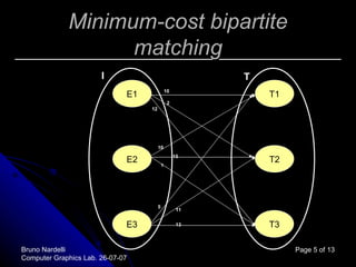
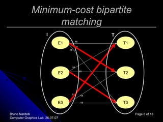
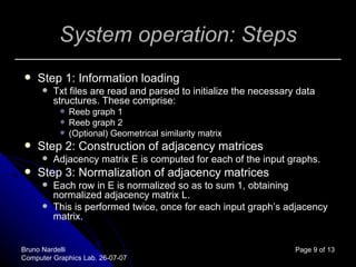
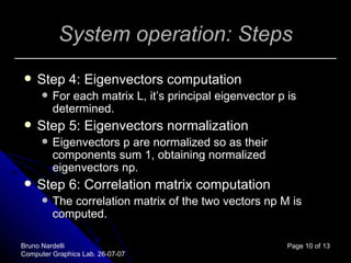
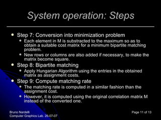
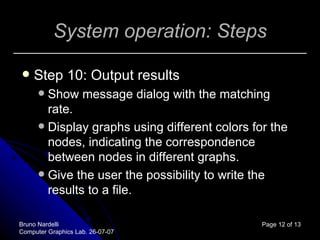
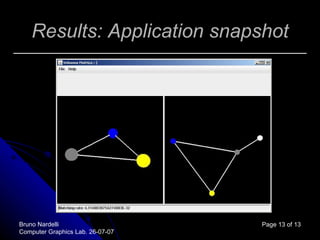
Graph Matching An implementation based on Khun-Munkres Algorithm
Problem description Consider two Reebgraphs describing topological features of two objects. The goal is to check for similarities between these two graphs and to return a possible assignment of correspondence between nodes in different graphs (graph matching). Page   of 13 Bruno Nardelli Computer Graphics Lab. 26-07-07
Problem description The problem is similar to that of finding isomorphisms and subisomorphisms between the graphs. However, to reduce the complexity of the algorithm we can reduce the original problem to a bipartite matching problem. This allows us to reuse existing algorithms for solving bipartite matching problem. One of these algorithms is the Khun-Munkres “Hungarian” Algorithm. Page   of 13 Bruno Nardelli Computer Graphics Lab. 26-07-07
Minimum-cost bipartite matching The typical example for understanding this problem considers a bipartite set with two classes (sets) of nodes Employees I Tasks T Each employee can perform a task with a different cost, according to his capabilities. The goal is to find an assignment (f: I    T) for which the overall cost is minimized. Page   of 13 Bruno Nardelli Computer Graphics Lab. 26-07-07
Minimum-cost bipartite matching Page   of 13 Bruno Nardelli Computer Graphics Lab. 26-07-07 E1 E2 E3 T1 T2 T3 10 15 10 2 1 12 11 5 13 I T
Minimum-cost bipartite matching The overall cost of an assignment f is the sum of the cost of (i, f(i)) for each element i in set I. For instance, in the previous example the overall assignment cost is 2+1+5 = 8. Since there exists no assignment with cost less than 8 for the given bipartite set. Page   of 13 Bruno Nardelli Computer Graphics Lab. 26-07-07
Formalization of the original problem Input: Txt file with the topological Reeb graph 1 enriched with geometrical information . Txt file with the topological Reeb graph 2 enriched with geometrical information . (Optional) Txt file with the geometrical similarity matrix between nodes in the two different graphs . Output: Matching rate as a number . Node-to-node correspondence . Graphical visualization of results. Page   of 13 Bruno Nardelli Computer Graphics Lab. 26-07-07
System operation: Steps Step 1: Information loading Txt files are read and parsed to initialize the necessary data structures .  These comprise: Reeb graph 1 Reeb graph 2 (Optional) Geometrical similarity matrix Step 2: Construction of adjacency matrices Adjacency matrix E is computed for each of the input graphs. Step 3: Normalization of adjacency matrices Each row in E is normalized so as to sum 1, obtaining normalized adjacency matrix L. This is performed twice, once for each input graph’s adjacency matrix. Page   of 13 Bruno Nardelli Computer Graphics Lab. 26-07-07
System operation: Steps Step 4: Eigenvectors computation For each matrix L, it’s principal eigenvector p is determined. Step 5: Eigenvectors normalization Eigenvectors p are normalized so as their components sum 1, obtaining normalized eigenvectors np. Step 6: Correlation matrix computation The correlation matrix of the two vectors np M is computed. Page   of 13 Bruno Nardelli Computer Graphics Lab. 26-07-07
System operation: Steps Step 7: Conversion into minimization problem Each element in M is substracted to the maximum so as to obtain a suitable cost matrix for a minimum bipartite matching problem. New rows or columns are also added if necessary, to make the matrix become square. Step 8: Bipartite matching Apply Hungarian Algorithm using the entries in the obtained matrix as assignment costs. Step 9: Compute matching rate The matching rate is computed in a similar fashion than the assignment cost. However, it is computed using the original correlation matrix M instead of the converted one. Page   of 13 Bruno Nardelli Computer Graphics Lab. 26-07-07
System operation: Steps Step 10: Output results Show message dialog with the matching rate. Display graphs using different colors for the nodes, indicating the correspondence between nodes in different graphs. Give the user the possibility to write the results to a file. Page   of 13 Bruno Nardelli Computer Graphics Lab. 26-07-07
Results: Application snapshot Page   of 13 Bruno Nardelli Computer Graphics Lab. 26-07-07
Conclusions Hungarian algorithm can be considered an instance of a backtracking algorithm. A lot of attention must be paid to its implementation, specially in handling particular or exceptional cases. Graph matching is approximate, but fast, and can still give good results in many cases. Page   of 13 Bruno Nardelli Computer Graphics Lab. 26-07-07

Graph Matching

  • 1.
    Graph Matching Animplementation based on Khun-Munkres Algorithm
  • 2.
    Problem description Considertwo Reebgraphs describing topological features of two objects. The goal is to check for similarities between these two graphs and to return a possible assignment of correspondence between nodes in different graphs (graph matching). Page of 13 Bruno Nardelli Computer Graphics Lab. 26-07-07
  • 3.
    Problem description Theproblem is similar to that of finding isomorphisms and subisomorphisms between the graphs. However, to reduce the complexity of the algorithm we can reduce the original problem to a bipartite matching problem. This allows us to reuse existing algorithms for solving bipartite matching problem. One of these algorithms is the Khun-Munkres “Hungarian” Algorithm. Page of 13 Bruno Nardelli Computer Graphics Lab. 26-07-07
  • 4.
    Minimum-cost bipartite matchingThe typical example for understanding this problem considers a bipartite set with two classes (sets) of nodes Employees I Tasks T Each employee can perform a task with a different cost, according to his capabilities. The goal is to find an assignment (f: I  T) for which the overall cost is minimized. Page of 13 Bruno Nardelli Computer Graphics Lab. 26-07-07
  • 5.
    Minimum-cost bipartite matchingPage of 13 Bruno Nardelli Computer Graphics Lab. 26-07-07 E1 E2 E3 T1 T2 T3 10 15 10 2 1 12 11 5 13 I T
  • 6.
    Minimum-cost bipartite matchingPage of 13 Bruno Nardelli Computer Graphics Lab. 26-07-07 E1 E2 E3 T1 T2 T3 10 15 10 2 1 12 11 5 13 I T
  • 7.
    Minimum-cost bipartite matchingThe overall cost of an assignment f is the sum of the cost of (i, f(i)) for each element i in set I. For instance, in the previous example the overall assignment cost is 2+1+5 = 8. Since there exists no assignment with cost less than 8 for the given bipartite set. Page of 13 Bruno Nardelli Computer Graphics Lab. 26-07-07
  • 8.
    Formalization of theoriginal problem Input: Txt file with the topological Reeb graph 1 enriched with geometrical information . Txt file with the topological Reeb graph 2 enriched with geometrical information . (Optional) Txt file with the geometrical similarity matrix between nodes in the two different graphs . Output: Matching rate as a number . Node-to-node correspondence . Graphical visualization of results. Page of 13 Bruno Nardelli Computer Graphics Lab. 26-07-07
  • 9.
    System operation: StepsStep 1: Information loading Txt files are read and parsed to initialize the necessary data structures . These comprise: Reeb graph 1 Reeb graph 2 (Optional) Geometrical similarity matrix Step 2: Construction of adjacency matrices Adjacency matrix E is computed for each of the input graphs. Step 3: Normalization of adjacency matrices Each row in E is normalized so as to sum 1, obtaining normalized adjacency matrix L. This is performed twice, once for each input graph’s adjacency matrix. Page of 13 Bruno Nardelli Computer Graphics Lab. 26-07-07
  • 10.
    System operation: StepsStep 4: Eigenvectors computation For each matrix L, it’s principal eigenvector p is determined. Step 5: Eigenvectors normalization Eigenvectors p are normalized so as their components sum 1, obtaining normalized eigenvectors np. Step 6: Correlation matrix computation The correlation matrix of the two vectors np M is computed. Page of 13 Bruno Nardelli Computer Graphics Lab. 26-07-07
  • 11.
    System operation: StepsStep 7: Conversion into minimization problem Each element in M is substracted to the maximum so as to obtain a suitable cost matrix for a minimum bipartite matching problem. New rows or columns are also added if necessary, to make the matrix become square. Step 8: Bipartite matching Apply Hungarian Algorithm using the entries in the obtained matrix as assignment costs. Step 9: Compute matching rate The matching rate is computed in a similar fashion than the assignment cost. However, it is computed using the original correlation matrix M instead of the converted one. Page of 13 Bruno Nardelli Computer Graphics Lab. 26-07-07
  • 12.
    System operation: StepsStep 10: Output results Show message dialog with the matching rate. Display graphs using different colors for the nodes, indicating the correspondence between nodes in different graphs. Give the user the possibility to write the results to a file. Page of 13 Bruno Nardelli Computer Graphics Lab. 26-07-07
  • 13.
    Results: Application snapshotPage of 13 Bruno Nardelli Computer Graphics Lab. 26-07-07
  • 14.
    Conclusions Hungarian algorithmcan be considered an instance of a backtracking algorithm. A lot of attention must be paid to its implementation, specially in handling particular or exceptional cases. Graph matching is approximate, but fast, and can still give good results in many cases. Page of 13 Bruno Nardelli Computer Graphics Lab. 26-07-07