


![Graduation Project 2020
Section 02
82
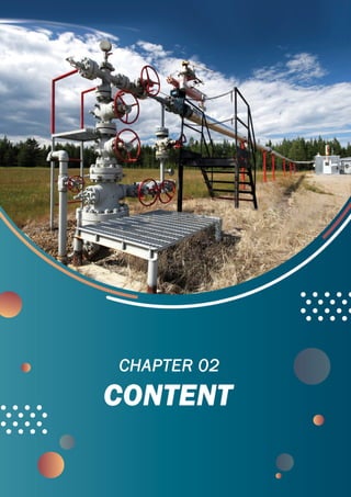
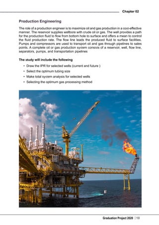
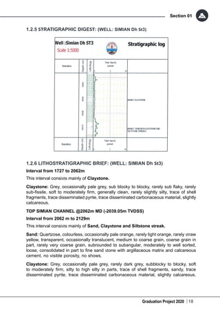
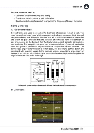
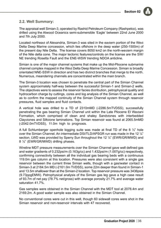
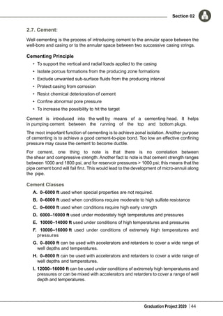
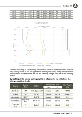
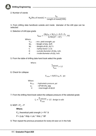
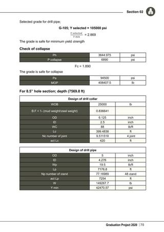
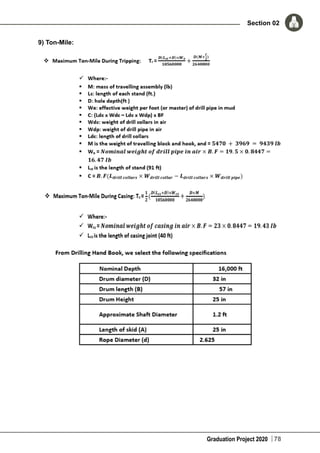
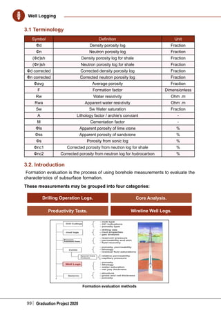
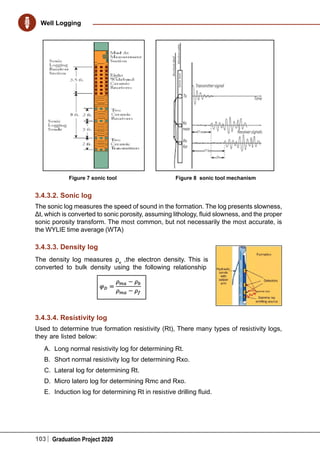
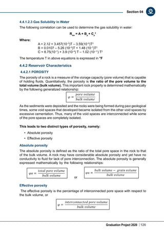
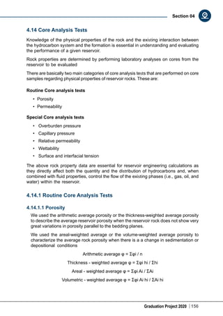
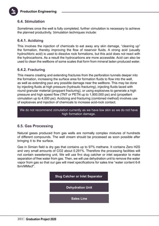
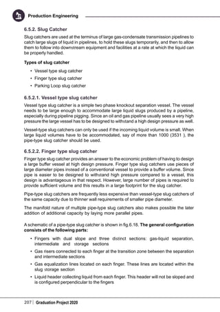
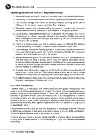
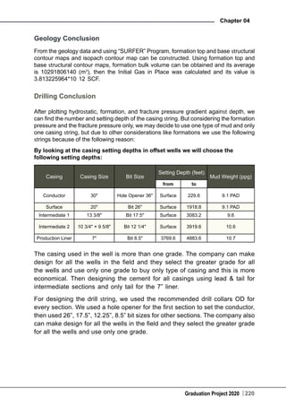
Drilling Instrumentation
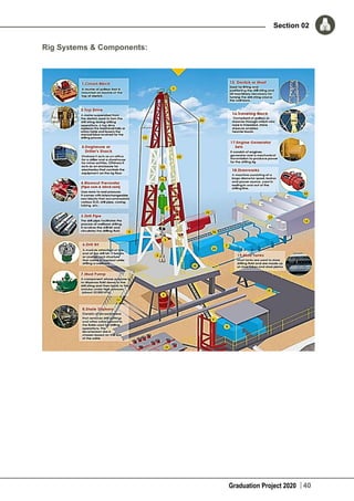
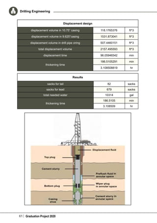
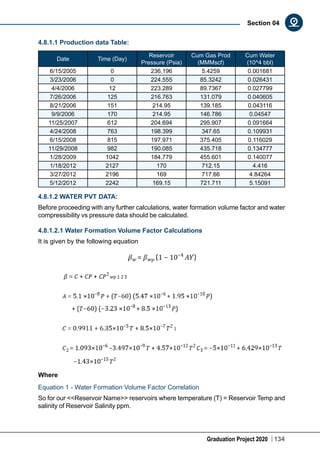
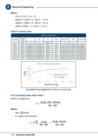
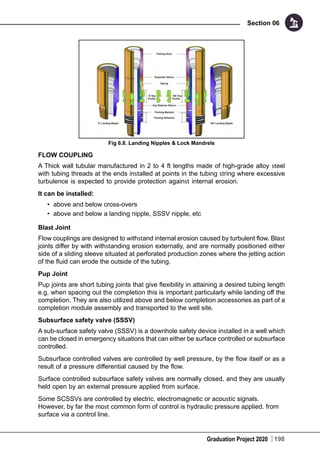
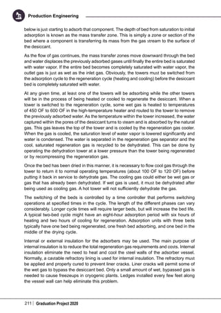
Petron driller cabin containing Petron Networked Distributed Drilling Data (3D)
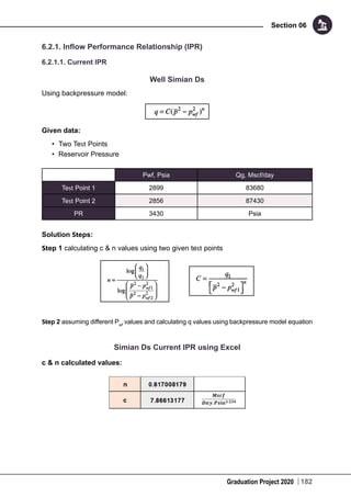
Instrumentation System consisting of:
1. Integrated drilling recorder function
2. Dual rig floor touch screen display with dual master panel capability
3. Drilling data hub monitoring:
a) Top drive torque f) Mud pump pressure (2) each
b) Top Drive RPM g) Cement pump pressure
c) Hydraulic hook load h) Casing/annular pressure
d) Hydraulic tong torque i) Flow sensor
e) Crown sensor depth and ROP
4. Mud pit data hub monitoring:
a) Riser boost pressure
b) Mud pump strokes (3 each)
c) Mud pit volume – thirteen (13) sensors in main mud pit system (three [3] pits
have dual sensors) and two (2) sensors in trip tank
5. Drilling data hub and Mud pit data hub are networked to workstation in Toolpusher’s
office and Company Rep’s office (optional)
6. Drillers console consisting of controls, gauges, and lights for the control and
monitoring of approximately 90 items
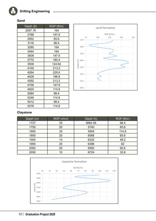
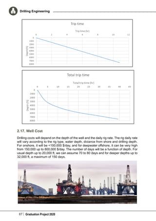
2.16. Graphically Plots
1) ROP](https://image.slidesharecdn.com/graduationbook2020-200811145324/85/Graduation-Project-Book-2020-86-320.jpg)


![105 Graduation Project 2020
Well Logging
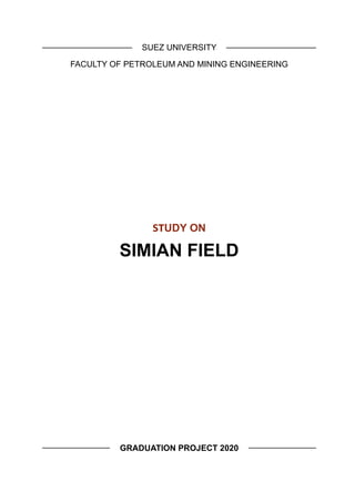
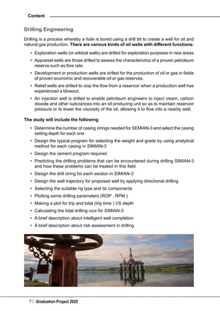
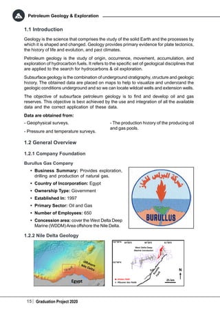
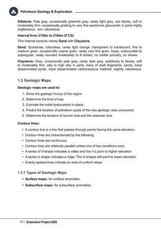
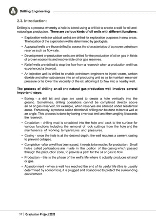
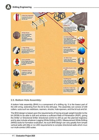
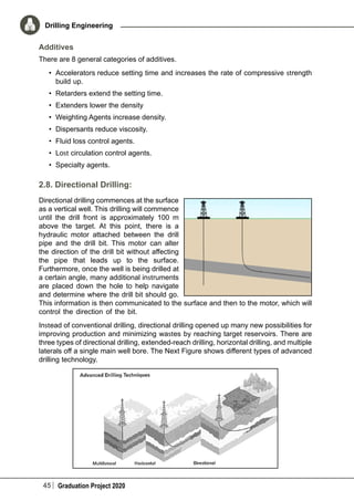
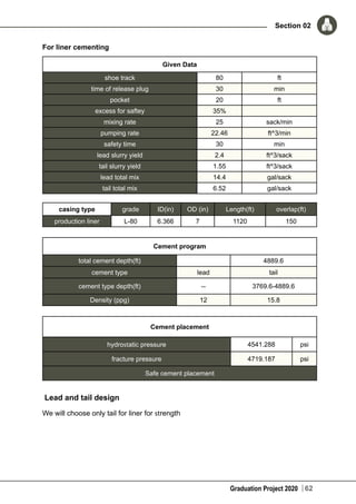
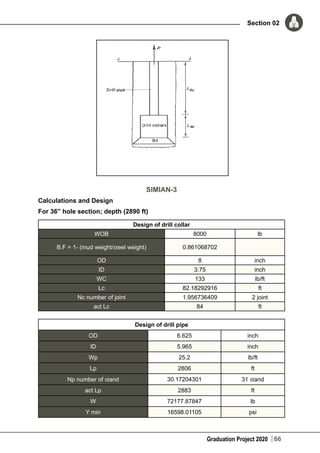
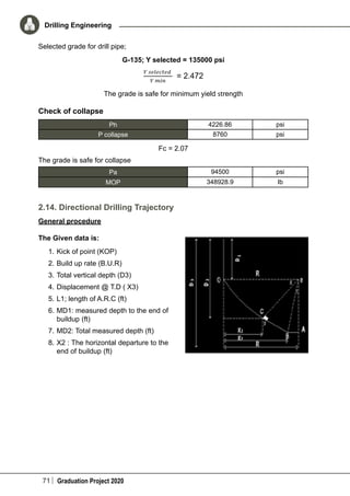
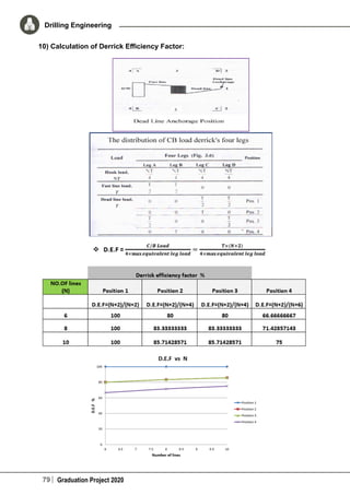
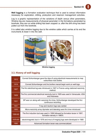
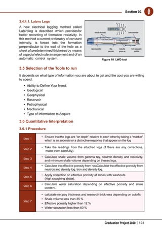
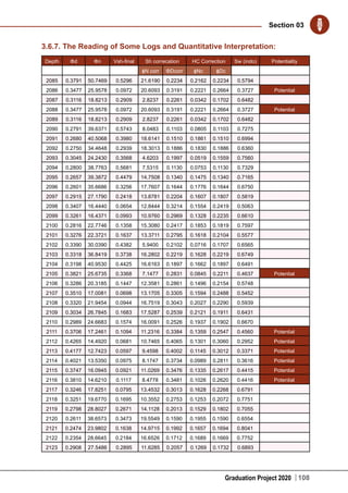
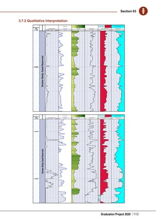
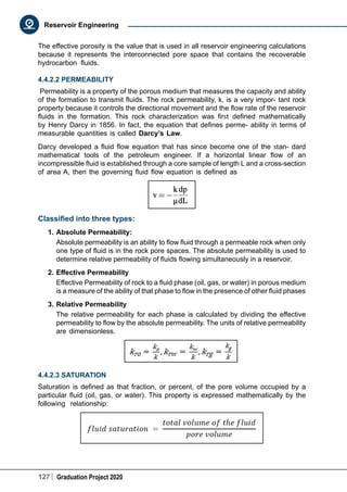
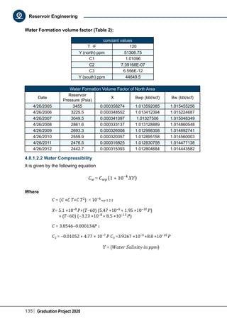
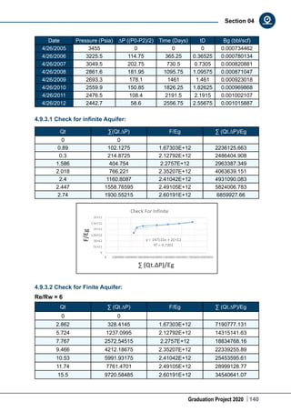
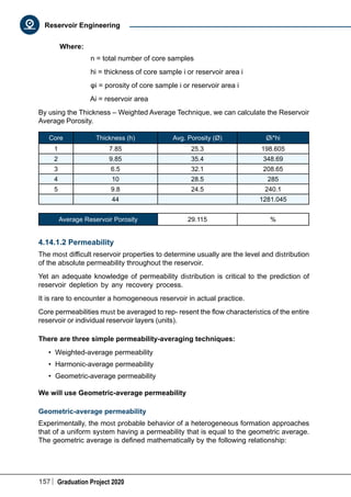
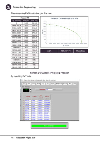
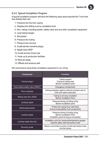
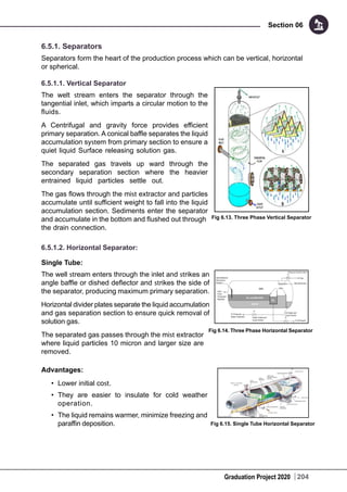
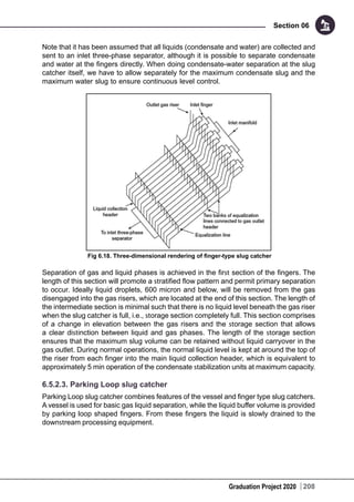
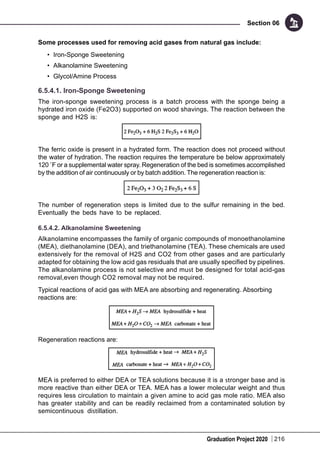
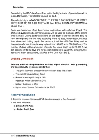
3.6.2. Correlations
3.6.2.1 Calculation of shale index (Ish):
From gamma ray log:
Where
Υ gamma ray response in the zone of interest.
γ min the average gamma ray response in the clean sand formation.
γ max the average gamma ray response in the cleanest shale formation
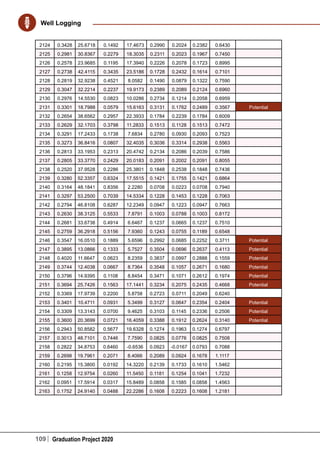
3.6.2.2 Calculation of Vshale (Vsh)
From gamma ray log:
- For linear relationship:
Vsh
= Ish
- For larionov equation for tertiary rocks
V = 0.083 × (23.7×Ish
− 1) sh
- For stieper equation
V =Ish
/(3−2Ish
)
- For older rocks, larionov equation
V = 0.33(22 Ish
− 1) sh
- For clavier et. Al equation
V = 1.7−[3.38−(I +0.7)2
]1/2
- From neutron porosity log
Where
Vsh
= (ØN
/ ØNsh
)
3.6.2.2.1 Density correction Neutron correction
ØN
Neutron porosity log reading at zone of interest.
ØNsh
Neutron porosity log reading opposite to the cleanest shale zone.
Porosities corrections
ØDC
= ØDC
− ØDSH
VSH
ØNC
= ØDC
− ØNSH
VSH
3.6.2.2.2 Correction for hydrocarbon effect
Light oil or gas will cause the formation density (ρb) to decrease by an amount of ∆ ρb &
apparent porosity (ØD & ØN) to increase by an amount of ( ∆ØD & ∆ØN ) respectively.](https://image.slidesharecdn.com/graduationbook2020-200811145324/85/Graduation-Project-Book-2020-109-320.jpg)


![Graduation Project 2020 136
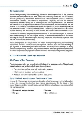
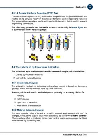
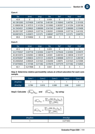
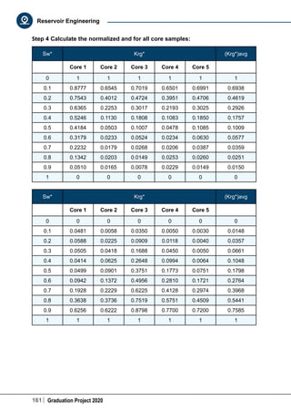
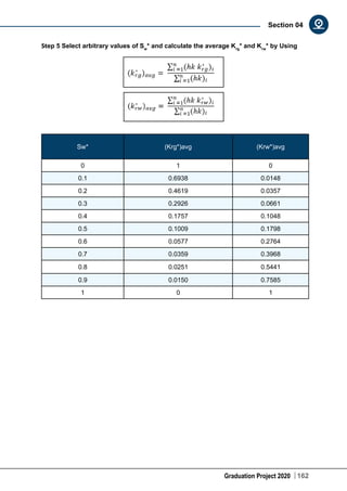
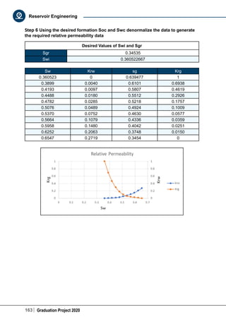
Section 04
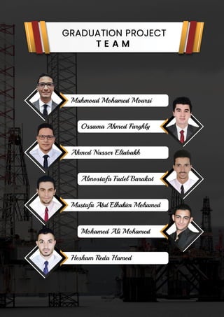
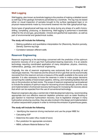
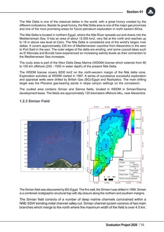
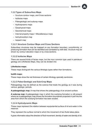
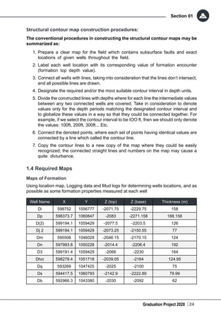
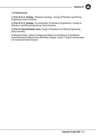
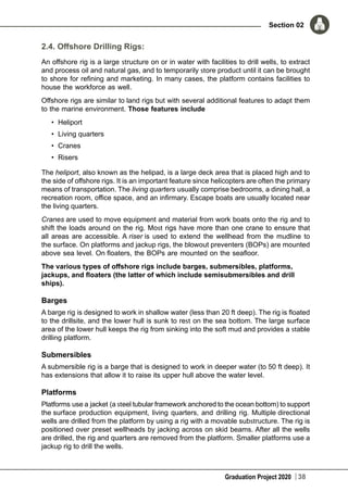
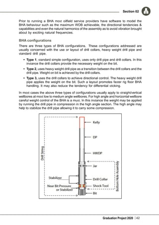
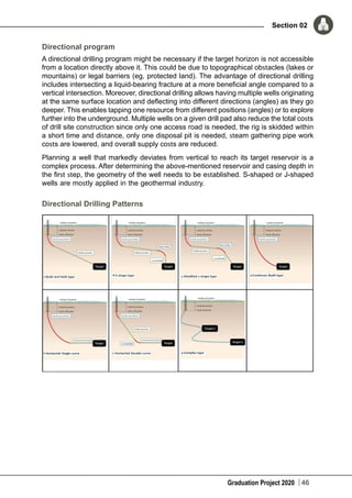
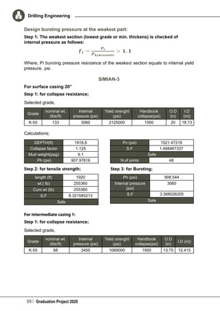
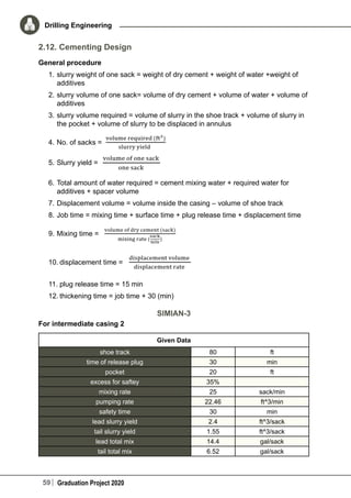
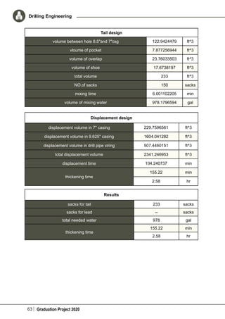
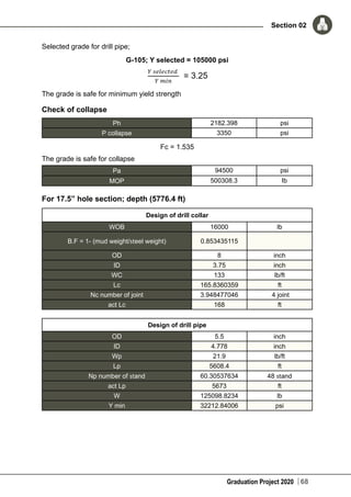
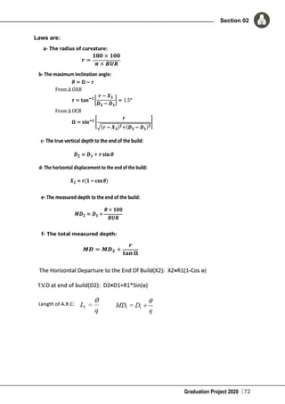
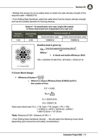
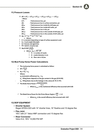
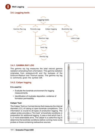
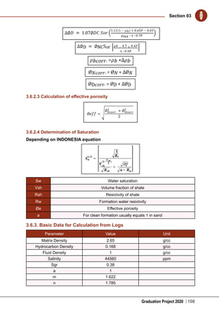
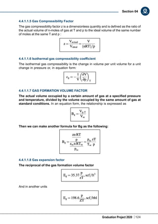
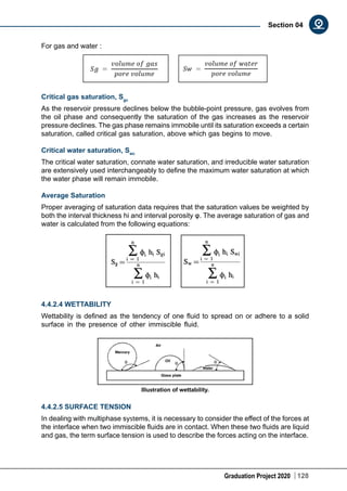
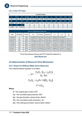
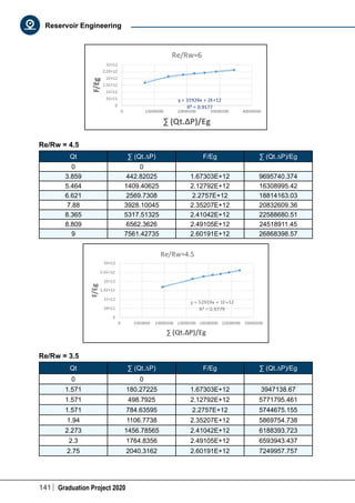
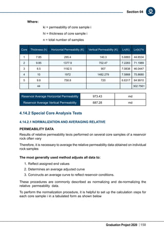
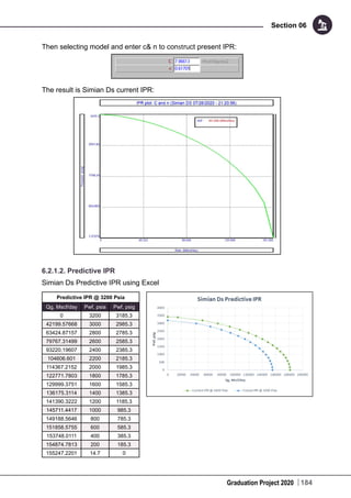
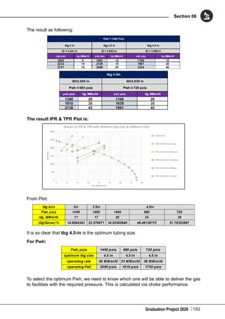
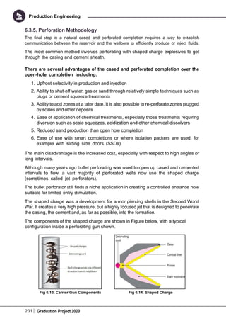
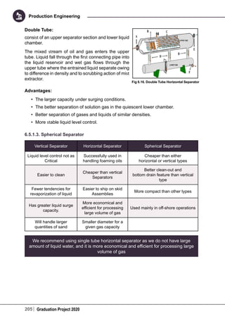
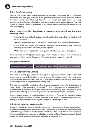
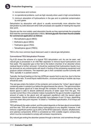
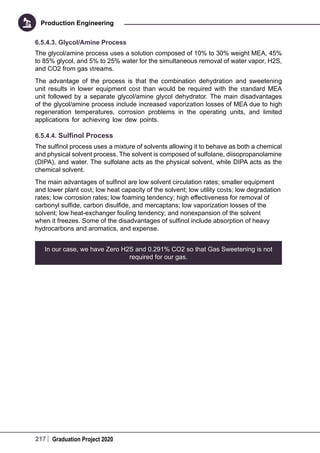
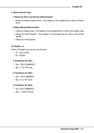
Water compressibility (Table 3):
Water Formation Volume Factor of North Area
Date
Reservoir
Pressure
C1 C2 C3 Cwp X Cw
4/26/2005 3455 3.39163 -0.008871965 3.62266E-05 2.76171E-06 0.000358274 2.76679E-06
4/26/2006 3225.5 3.422383 -0.008981437 3.64286E-05 2.78175E-06 0.000348552 2.78673E-06
4/26/2007 3049.5 3.445967 -0.009065389 3.65834E-05 2.79712E-06 0.000341097 2.80202E-06
4/26/2008 2861.6 3.4711456 -0.009155017 3.67488E-05 2.81353E-06 0.000333137 2.81834E-06
4/26/2009 2693.3 3.4936978 -0.009235296 3.68969E-05 2.82823E-06 0.000326008 2.83296E-06
4/26/2010 2559.9 3.5115734 -0.009298928 3.70143E-05 2.83987E-06 0.000320357 2.84454E-06
4/26/2011 2476.5 3.522749 -0.00933871 3.70877E-05 2.84716E-06 0.000316825 2.85178E-06
4/26/2012 2442.7 3.5272782 -0.009354832 3.71174E-05 2.85011E-06 0.000315393 2.85472E-06
4.8.1.2.3 Water Viscosity:
μw = μwD*[1+3.5*10^-2*P^-2*(T-40)]
Where
μwD = A+B/T
A = 4.518*10^-2+9.313*10^-7*Y-3.93*10^-12*Y^2
B = 70.634+9.576*10^-10*Y^2
Where
μw = brine viscosity at P and T,CP
μwD = brine viscosity at P=14.7,T,CP
P = Reservoir pressure, Psi
T = reservoir temperature
Y = Water Salinity.ppm
Water Viscosity of North Area
Date Reservoir Pressure (Psia) μw
4/26/2005 3455 20117032.16
4/26/2006 3225.5 17533228.84
4/26/2007 3049.5 15672023.92
4/26/2008 2861.6 13800209.11
4/26/2009 2693.3 12224673.75
4/26/2010 2559.9 11043680.11
4/26/2011 2476.5 10335809.2
4/26/2012 2442.7 10055602.21
constant values (north)
T ͦF 120
A -0.007743287
B 73.15476957
μwD 0.601879792](https://image.slidesharecdn.com/graduationbook2020-200811145324/85/Graduation-Project-Book-2020-140-320.jpg)
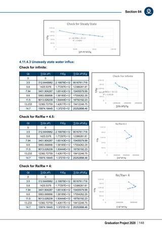
![Graduation Project 2020 146
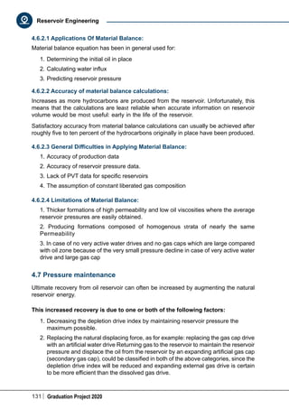
Section 04
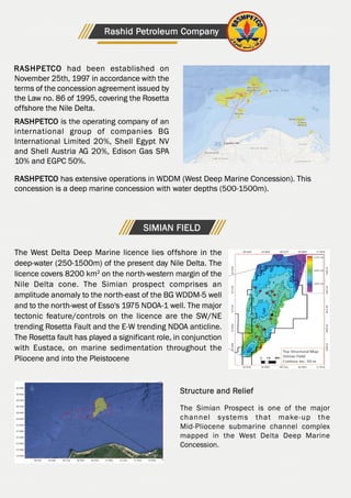
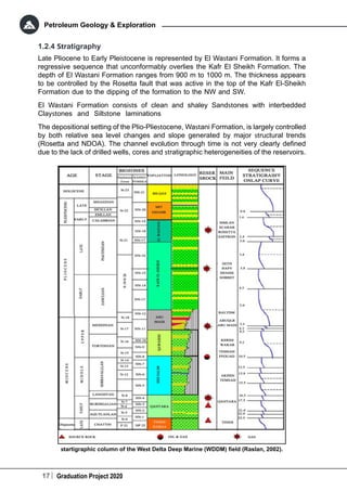
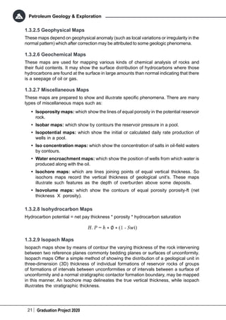
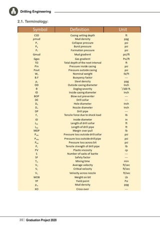
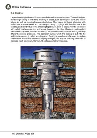
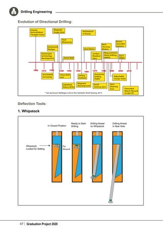
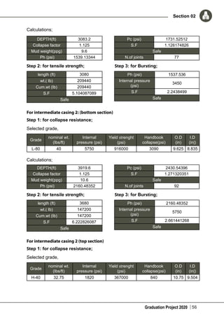
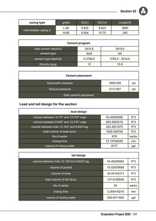
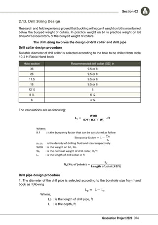
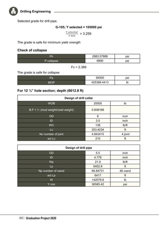
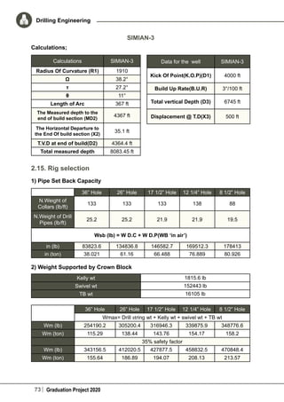
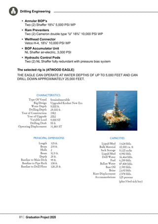
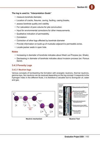
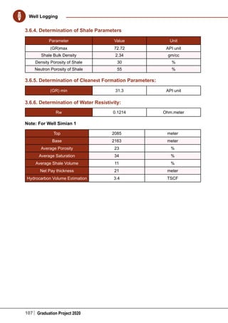
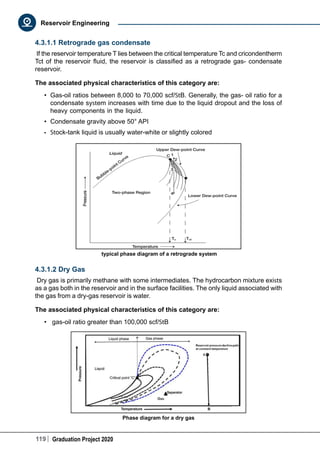
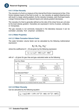
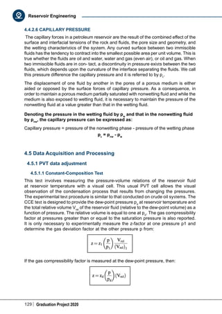
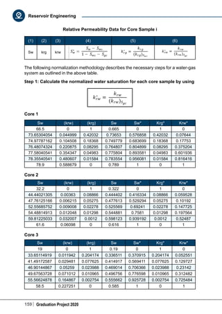
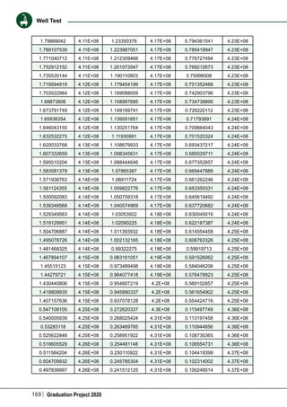
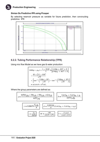
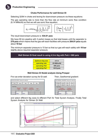
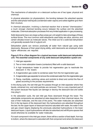
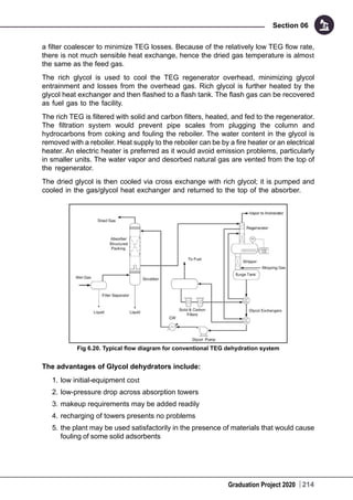
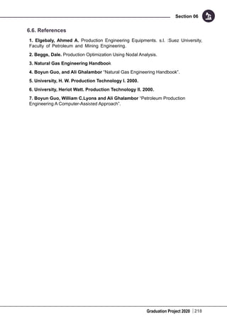
4.11.2.2 Wate compressibility:
Cw =Cwp * (1+X*Y*10^-4)
Date
Reservoir
Pressure psia
C1 C2 C3 Cwp X Cw
4/26/2005 3455 3.39163 -0.008872 3.623E-05 2.762E-06 1.762E+12 21727684
4/26/2006 3276.345715 3.4155697 -0.0089572 3.638E-05 2.777E-06 1.671E+12 20720556
4/26/2007 2936.462757 3.461114 -0.0091193 3.668E-05 2.807E-06 1.498E+12 18769489
4/26/2008 2596.980702 3.5066046 -0.0092812 3.698E-05 2.837E-06 1.324E+12 16774866
4/26/2009 2304.018793 3.5458615 -0.009421 3.724E-05 2.862E-06 1.175E+12 15016730
4/26/2010 2045.198566 3.5805434 -0.0095444 3.747E-05 2.885E-06 1.043E+12 13435089
4/26/2011 1819.933325 3.6107289 -0.0096519 3.767E-05 2.904E-06 9.282E+11 12036820
4/26/2012 1648.81514 3.6336588 -0.0097335 3.782E-05 2.919E-06 8.409E+11 10961165
4/26/2013 1444.934097 3.6609788 -0.0098308 3.8E-05 2.937E-06 7.369E+11 9664360.4
4/26/2014 1308.396909 3.6792748 -0.0098959 3.812E-05 2.949E-06 6.673E+11 8786660.6
4/26/2015 1251.874266 3.6868488 -0.0099229 3.817E-05 2.954E-06 6.385E+11 8421147.2
4.11.2.3 Water Viscosity:
μw= μwD*[1+3.5*10^-2*P^-2*(T-40)]
Water Viscosity
Date Reservoir Pressure psia μw cp
4/26/2005 3455 19823336.49
4/26/2006 3276.345715 17826254.16
4/26/2007 2936.462757 14319559.18
4/26/2008 2596.980702 11200002.11
4/26/2009 2304.018793 8815616.721
4/26/2010 2045.198566 6946269.561
4/26/2011 1819.933325 5500366.624
4/26/2012 1648.81514 4514655.613
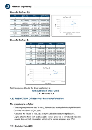
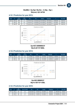
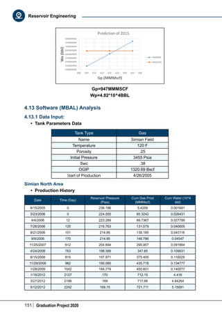
4.11.3 PVT Data for Gas:
Constant Values
T F Tpc R Tpr Ppc psia SP.Gr µ1 N2 µ2 CO2 µ1 HC µ1 Y N2 Y CO2 Y N2 Y CO2
120 349.18875 1.6609928 663.36625 0.57 1.181E-05 1.171E-05 0.0115991 0.0116226 0.00157 0.00291 0.002 0.003
a0 a1 a2 a3 a4 a5 a6 a7 a8 a9 a10 a11 a12
-2.4621 2.9705 -0.2862 0.008 2.8086 -3.498 0.3603 -0.0104 -0.7933 1.3964 -0.1491 0.004 0.084
a11 a12 a13 a14 a15
0.0044 0.0839 -0.1864 0.0203 -0.0006](https://image.slidesharecdn.com/graduationbook2020-200811145324/85/Graduation-Project-Book-2020-150-320.jpg)


![Graduation Project 2020
Section 05
178
5.5. References:
1. Advanced Reservoir Engineering,Tarek Ahmed & Paul D.McKinney.
2. Applied Well Test Interpretation, John P.Spivey& W. John Lee.
3. Modern Well Test Analysis (A computer-Aided approach).
4. Well Testing (SPE Textbook Series Vol.1 ) [John Lee].
5. SPETextbookSeries_Volume9_PressureTransientTesting.](https://image.slidesharecdn.com/graduationbook2020-200811145324/85/Graduation-Project-Book-2020-182-320.jpg)


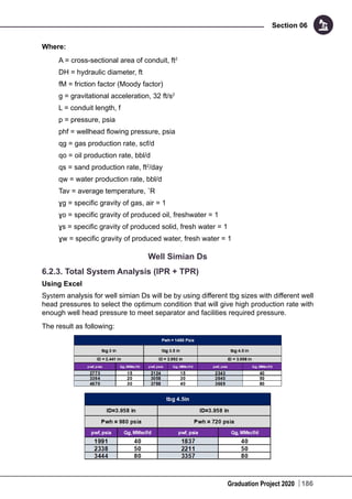
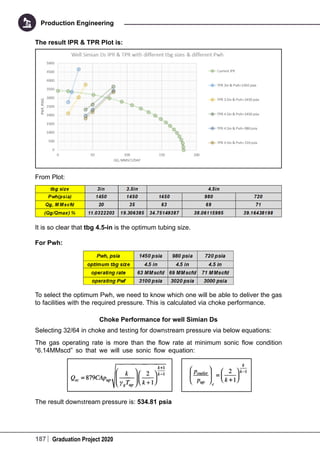
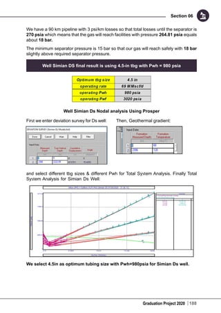
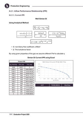
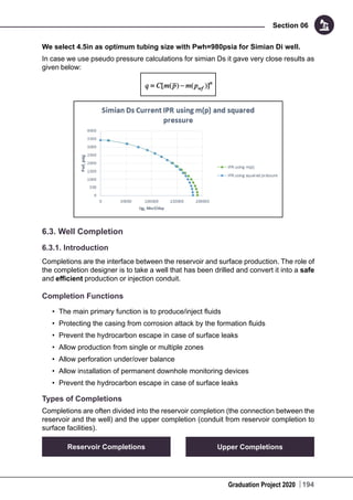


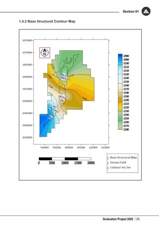
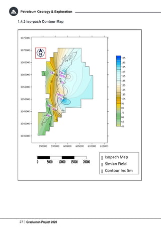
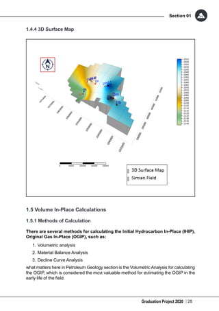
This document provides an overview of a graduation project studying the SIMIAN field. It will integrate petroleum geology and exploration, drilling engineering, well logging, reservoir engineering, well testing, and production engineering. The study will include constructing structure contour maps, isopach maps, and calculating the original gas in place. It will also include determining the number of casing strings needed, designing the cement program, predicting drilling problems, and calculating the total drilling cost. Other aspects covered are making qualitative and quantitative log interpretations, identifying the reservoir driving mechanism, determining boundaries and properties from well testing, and selecting the optimum tubing size and gas processing method.