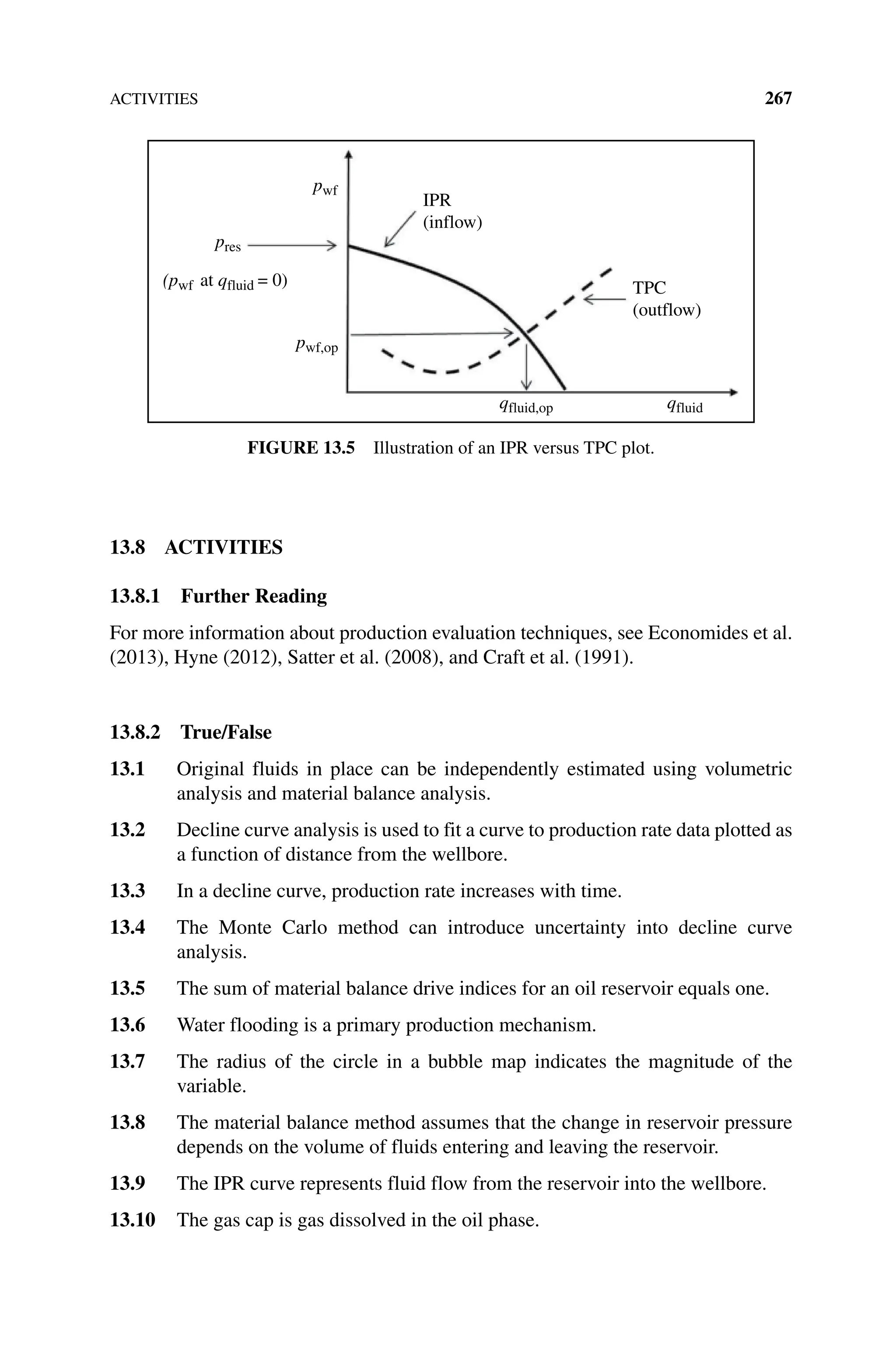
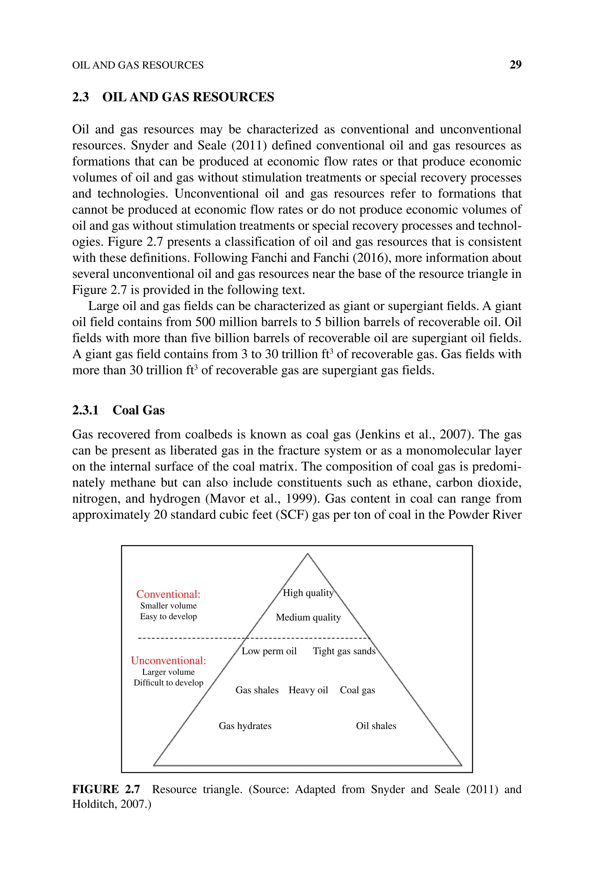
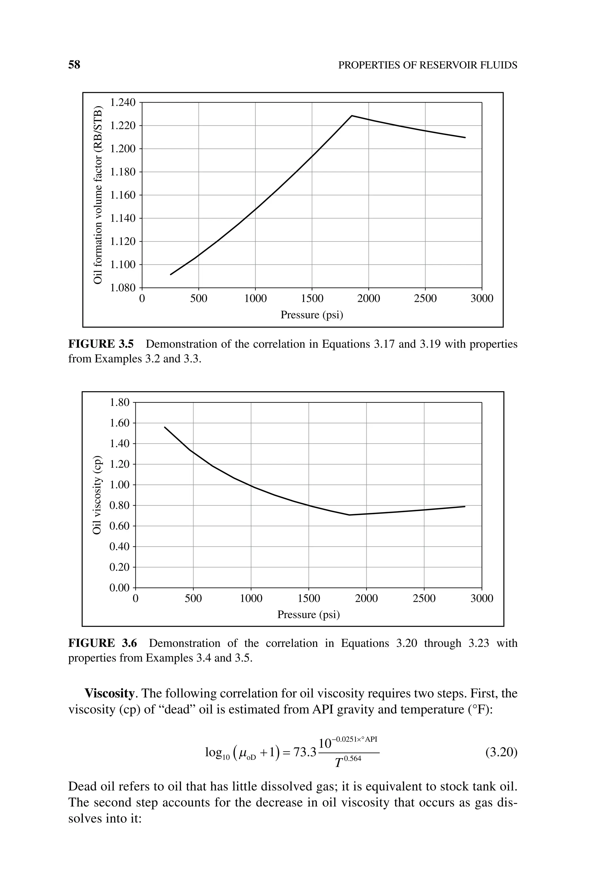
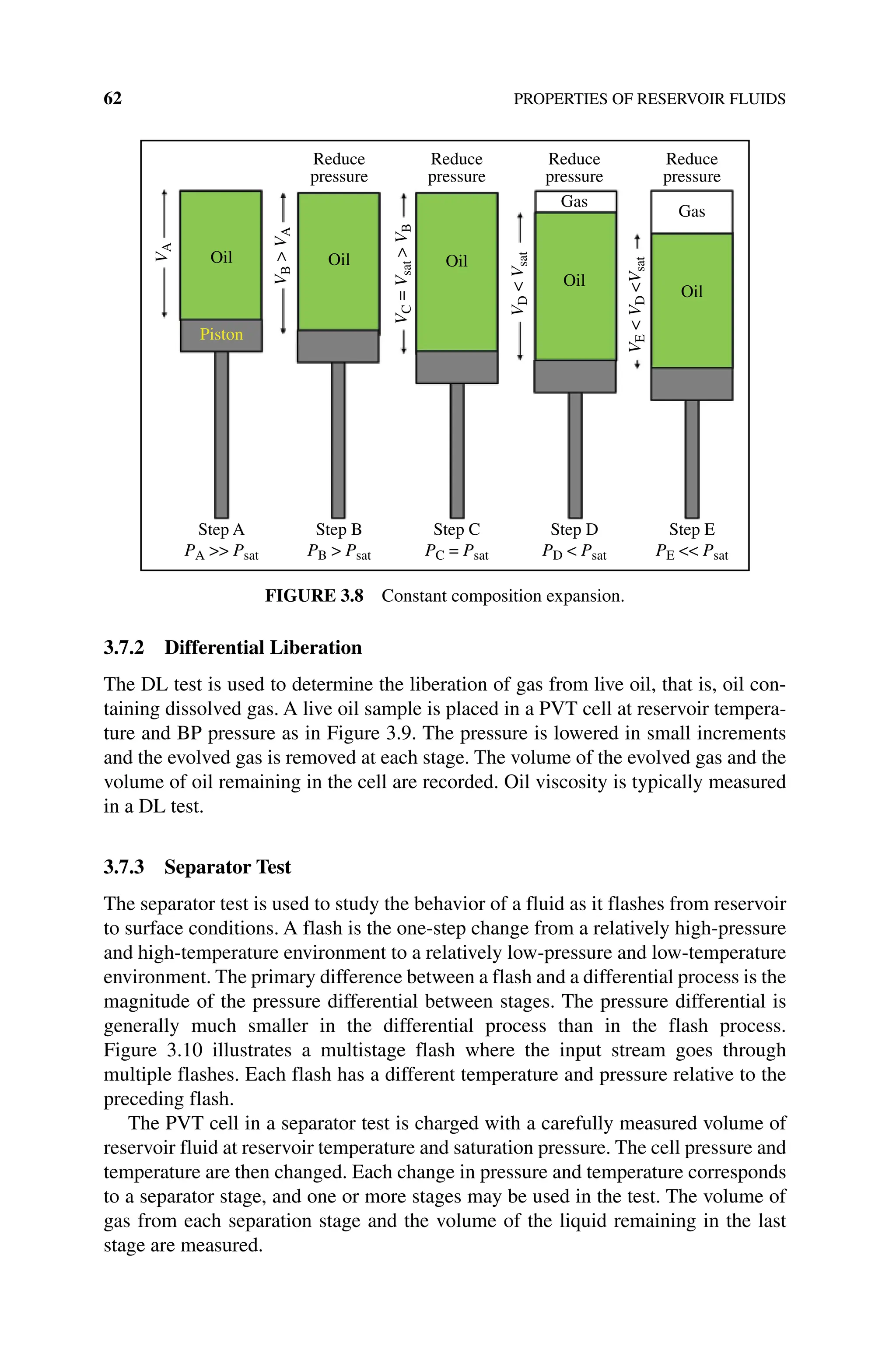
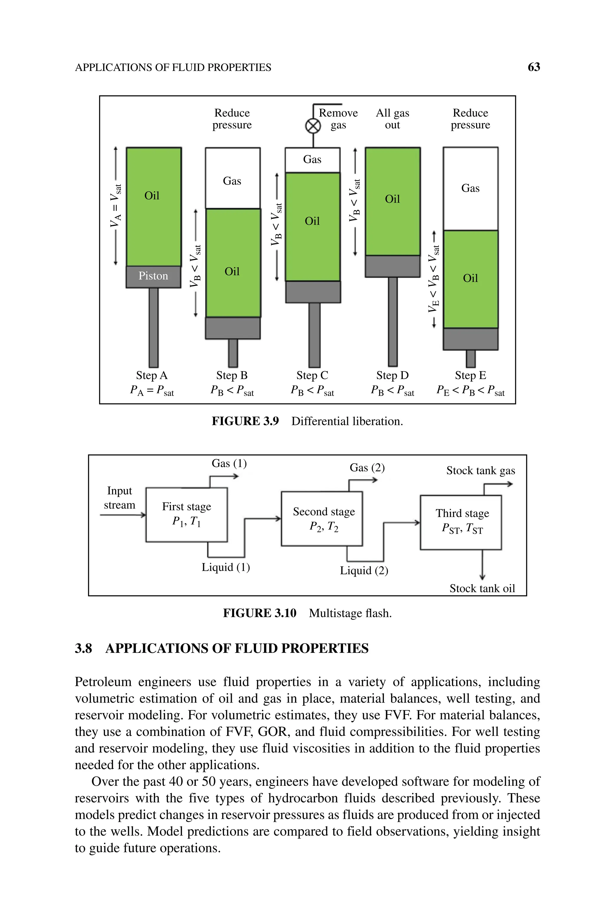
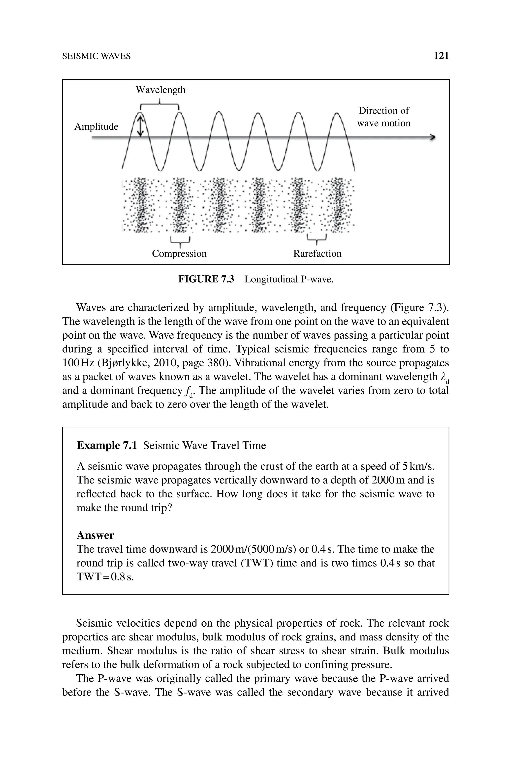
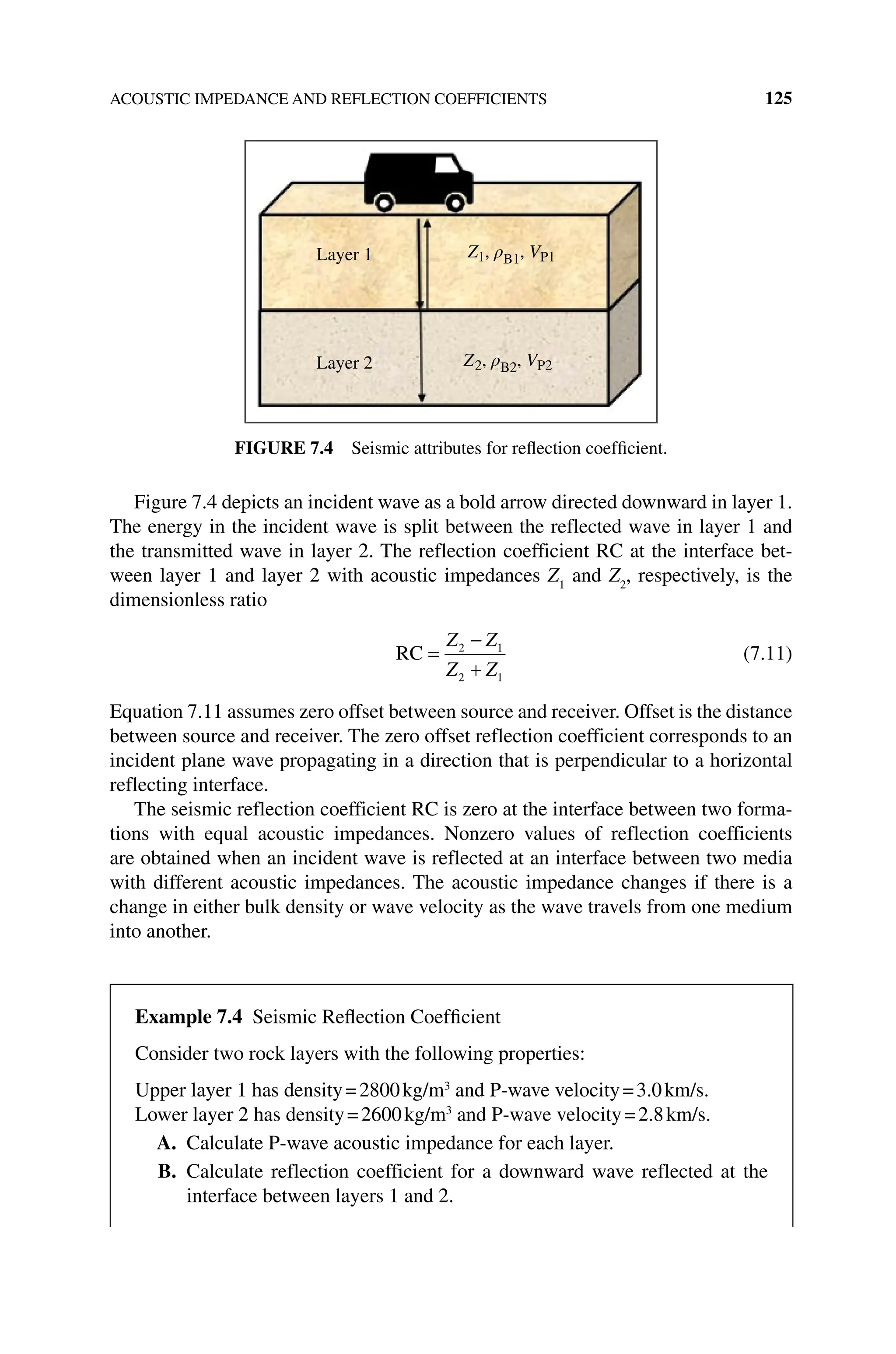
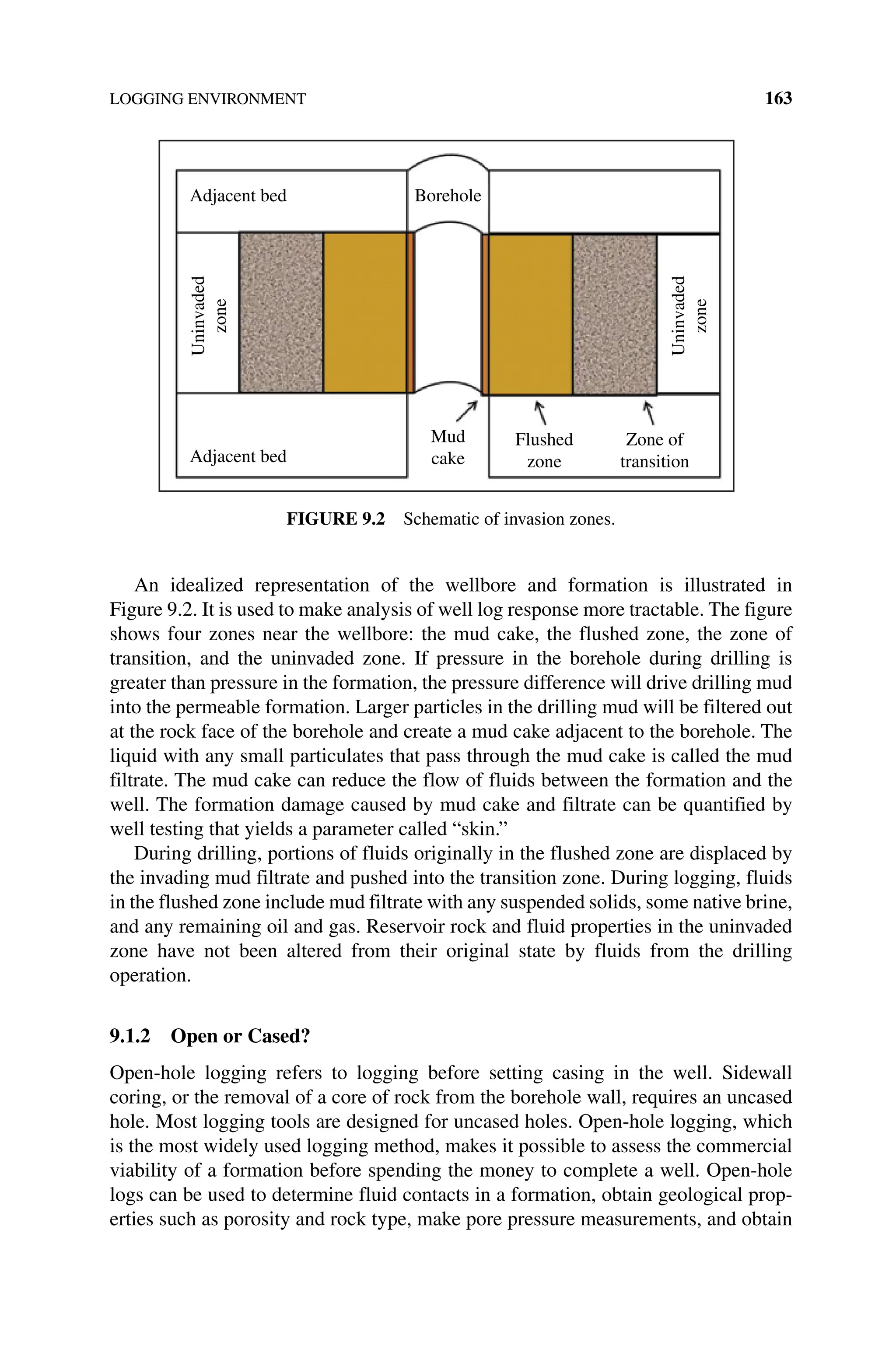
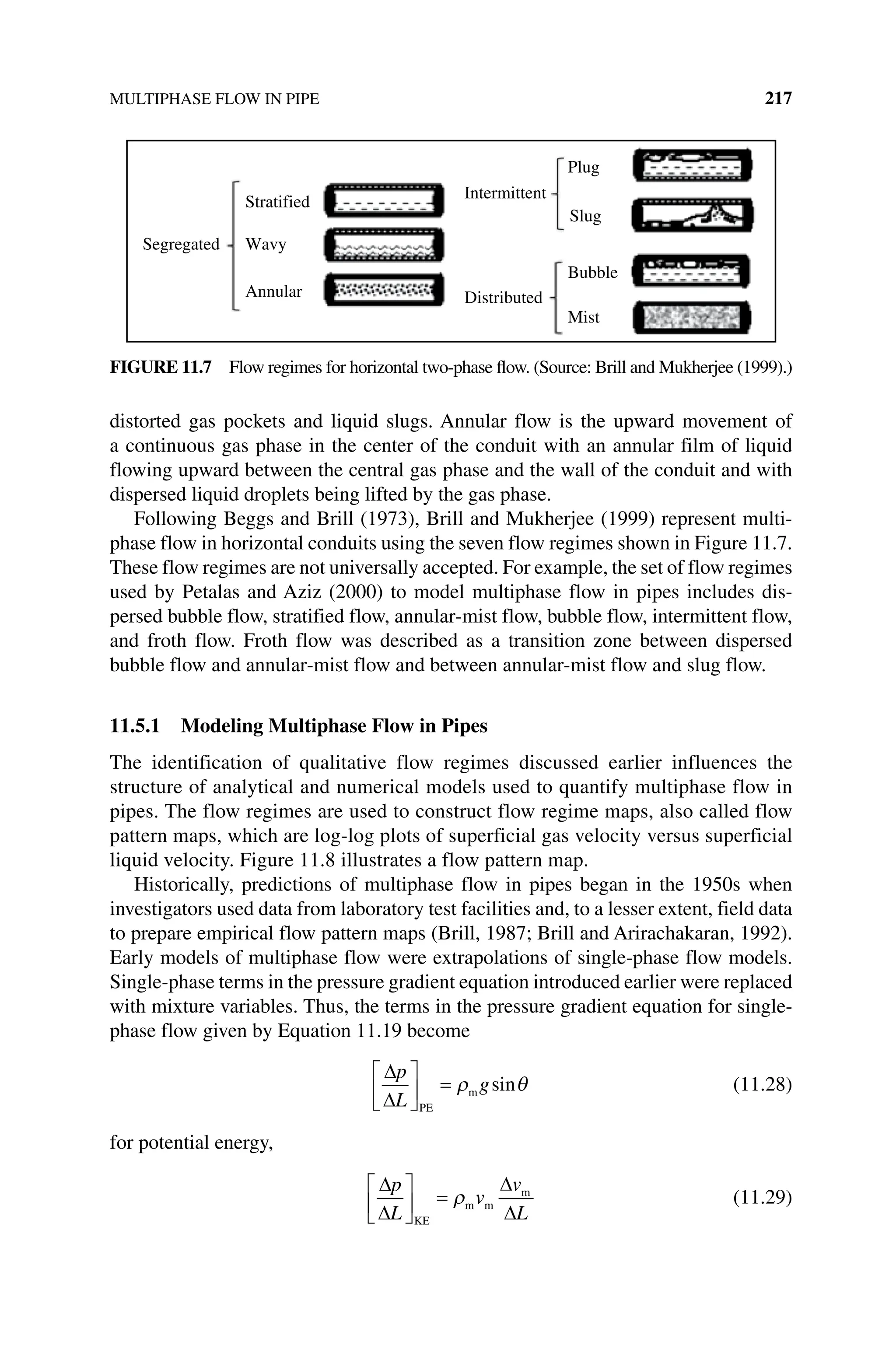
The document is a comprehensive introduction to petroleum engineering authored by John R. Fanchi and Richard L. Christiansen, detailing key concepts such as reservoir management, production performance, and the future of energy. It covers various aspects of the field, including drilling, well logging, and production performance, alongside practical activities and further readings for educational purposes. The book stresses the importance of environmental considerations and economics in relation to petroleum engineering.

![Copyright © 2017 by John Wiley & Sons, Inc. All rights reserved
Published by John Wiley & Sons, Inc., Hoboken, New Jersey
Published simultaneously in Canada
No part of this publication may be reproduced, stored in a retrieval system, or transmitted in any form
or by any means, electronic, mechanical, photocopying, recording, scanning, or otherwise, except as
permitted under Section 107 or 108 of the 1976 United States Copyright Act, without either the prior
written permission of the Publisher, or authorization through payment of the appropriate per‐copy fee
to the Copyright Clearance Center, Inc., 222 Rosewood Drive, Danvers, MA 01923, (978) 750‐8400,
fax (978) 750‐4470, or on the web at www.copyright.com. Requests to the Publisher for
permission should be addressed to the Permissions Department, John Wiley & Sons, Inc.,
111 River Street, Hoboken, NJ 07030, (201) 748‐6011, fax (201) 748‐6008, or online at
http://www.wiley.com/go/permissions.
Limit of Liability/Disclaimer of Warranty: While the publisher and author have used their best efforts
in preparing this book, they make no representations or warranties with respect to the accuracy or
completeness of the contents of this book and specifically disclaim any implied warranties of
merchantability or fitness for a particular purpose. No warranty may be created or extended by sales
representatives or written sales materials. The advice and strategies contained herein may not be suitable
for your situation. You should consult with a professional where appropriate. Neither the publisher nor
author shall be liable for any loss of profit or any other commercial damages, including but not limited to
special, incidental, consequential, or other damages.
For general information on our other products and services or for technical support, please contact our
Customer Care Department within the United States at (800) 762‐2974, outside the United States at
(317) 572‐3993 or fax (317) 572‐4002.
Wiley also publishes its books in a variety of electronic formats. Some content that appears in print may
not be available in electronic formats. For more information about Wiley products, visit our web site at
www.wiley.com.
Library of Congress Cataloging‐in‐Publication Data:
Names: Fanchi, John R., author. | Christiansen, Richard L. (Richard Lee), author.
Title: Introduction to petroleum engineering / by John R. Fanchi and Richard L. Christiansen.
Description: Hoboken, New Jersey : John Wiley & Sons, Inc., [2017] | Includes bibliographical
references and index.
Identifiers: LCCN 2016019048| ISBN 9781119193449 (cloth) | ISBN 9781119193647 (epdf) |
ISBN 9781119193616 (epub)
Subjects: LCSH: Petroleum engineering.
Classification: LCC TN870 .F327 2017 | DDC 622/.3382–dc23
LC record available at https://lccn.loc.gov/2016019048
Printed in the United States of America
10 9 8 7 6 5 4 3 2 1](https://image.slidesharecdn.com/introductiontopetroleumengineeringbyjohnr-241125084112-ea228c08/75/Introduction-to-Petroleum-Engineering-by-John-R-Fanchi-pdf-3-2048.jpg)


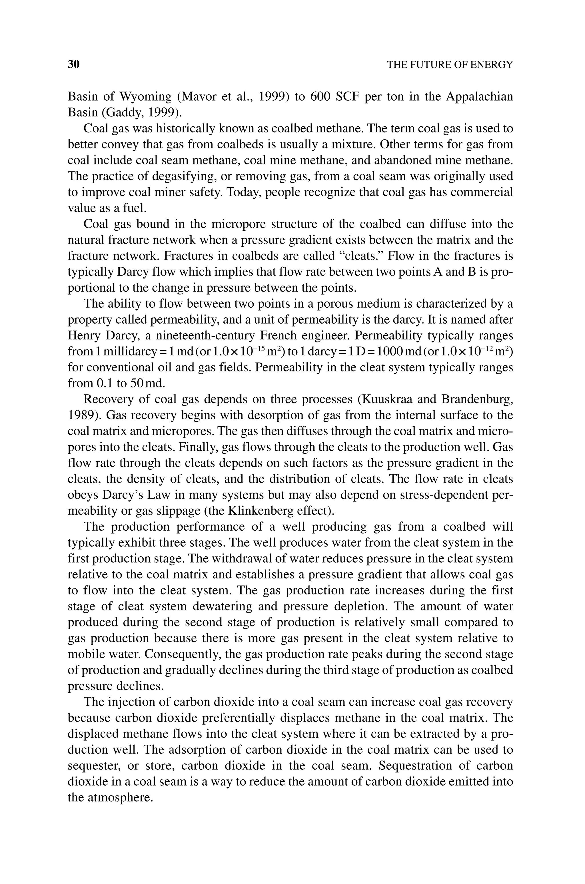

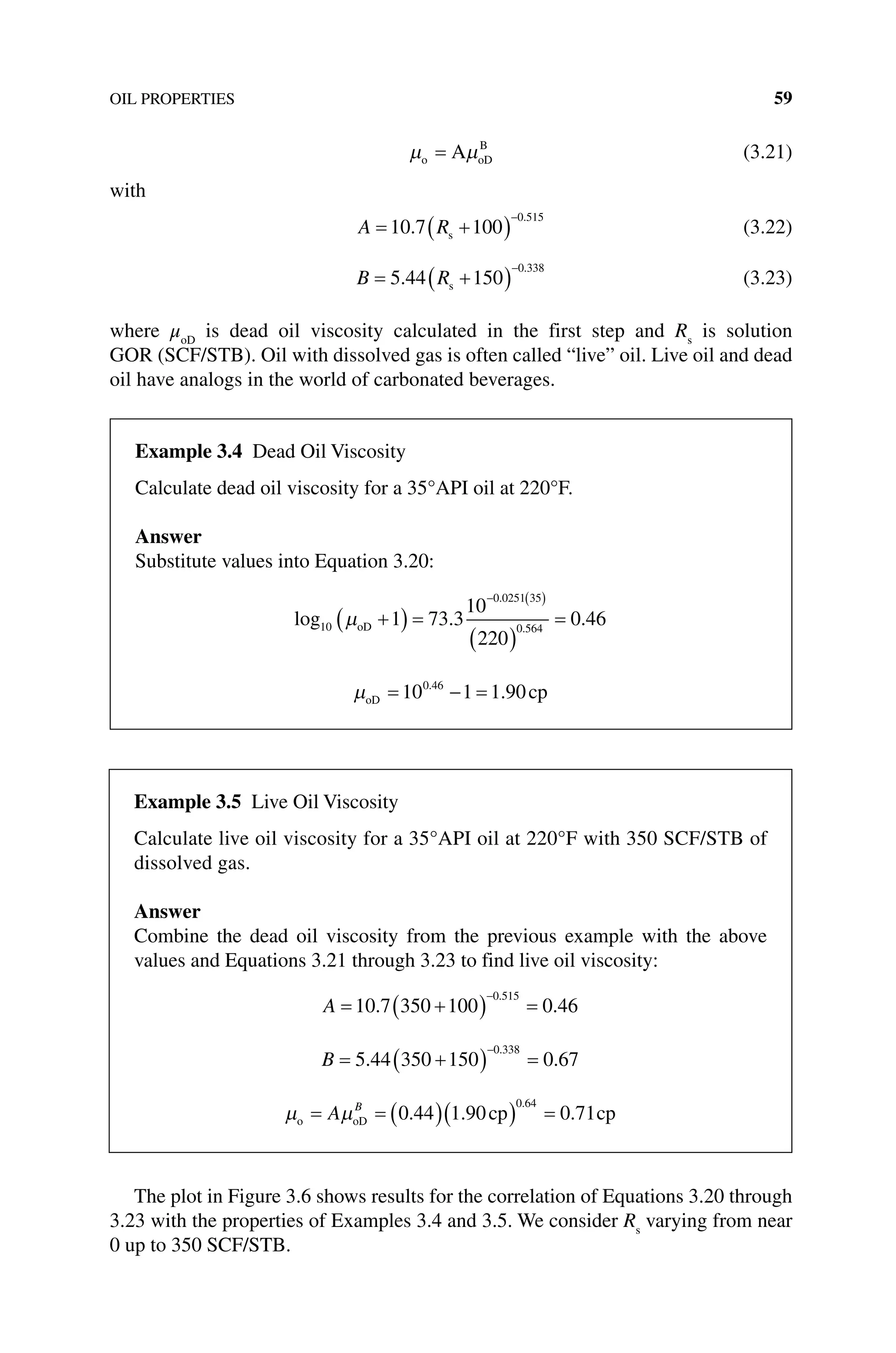

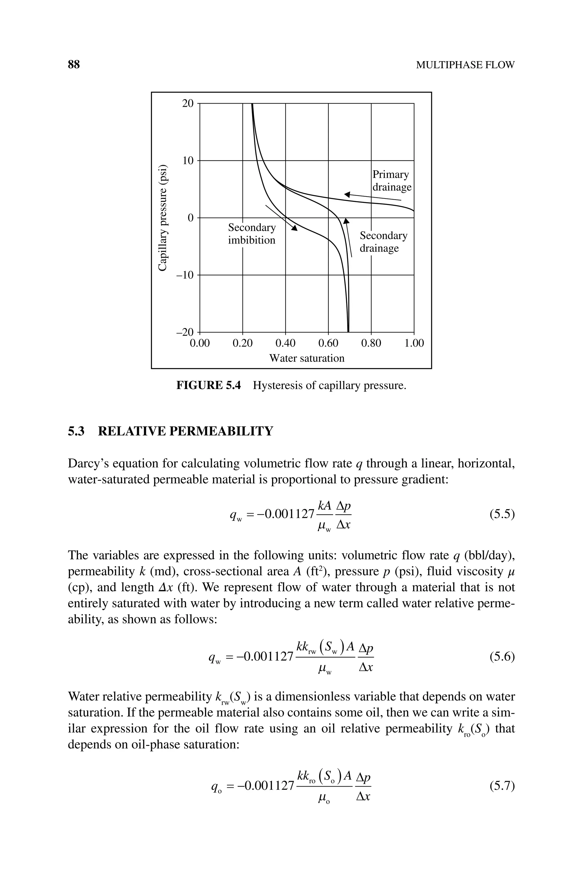
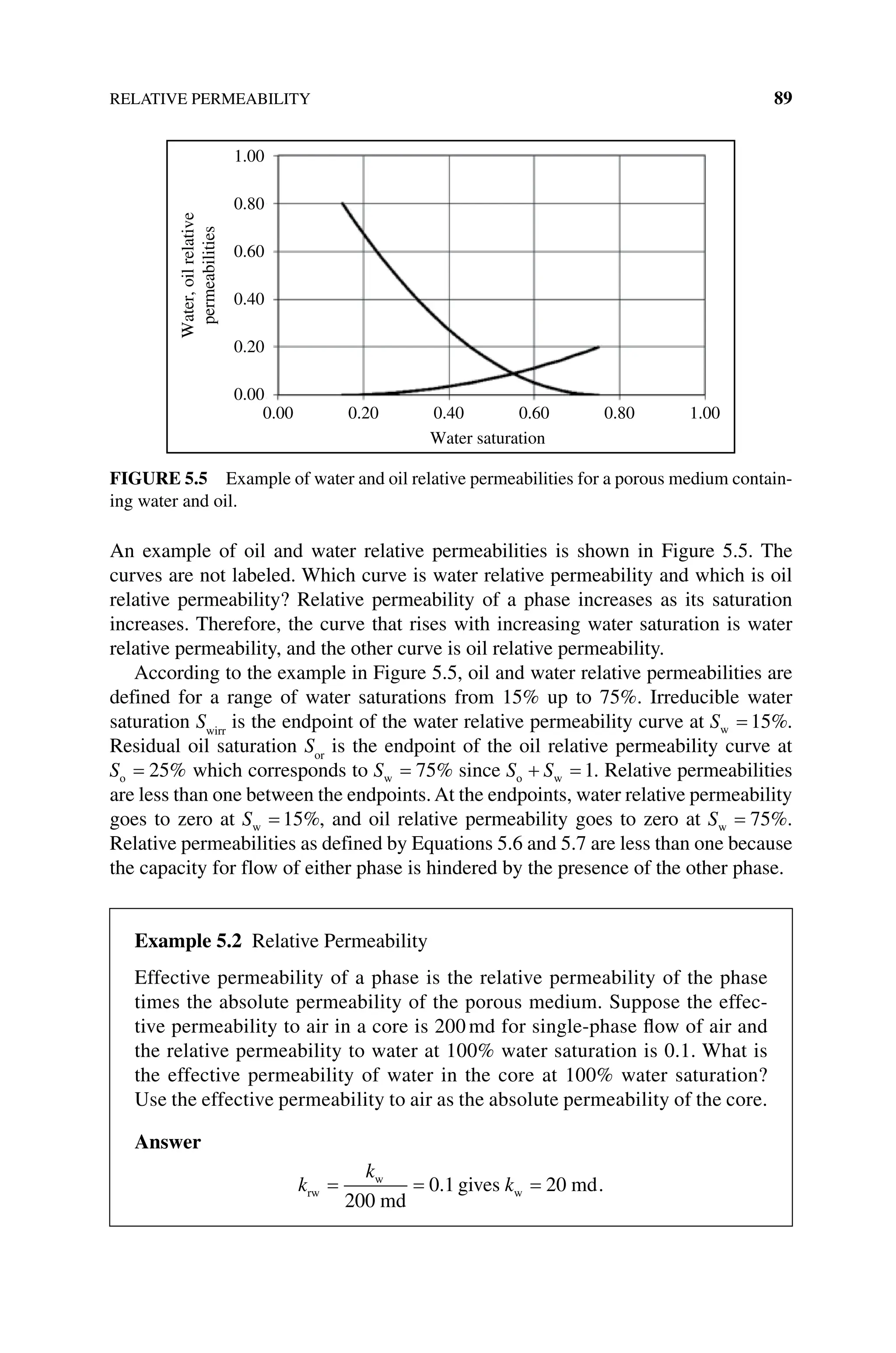
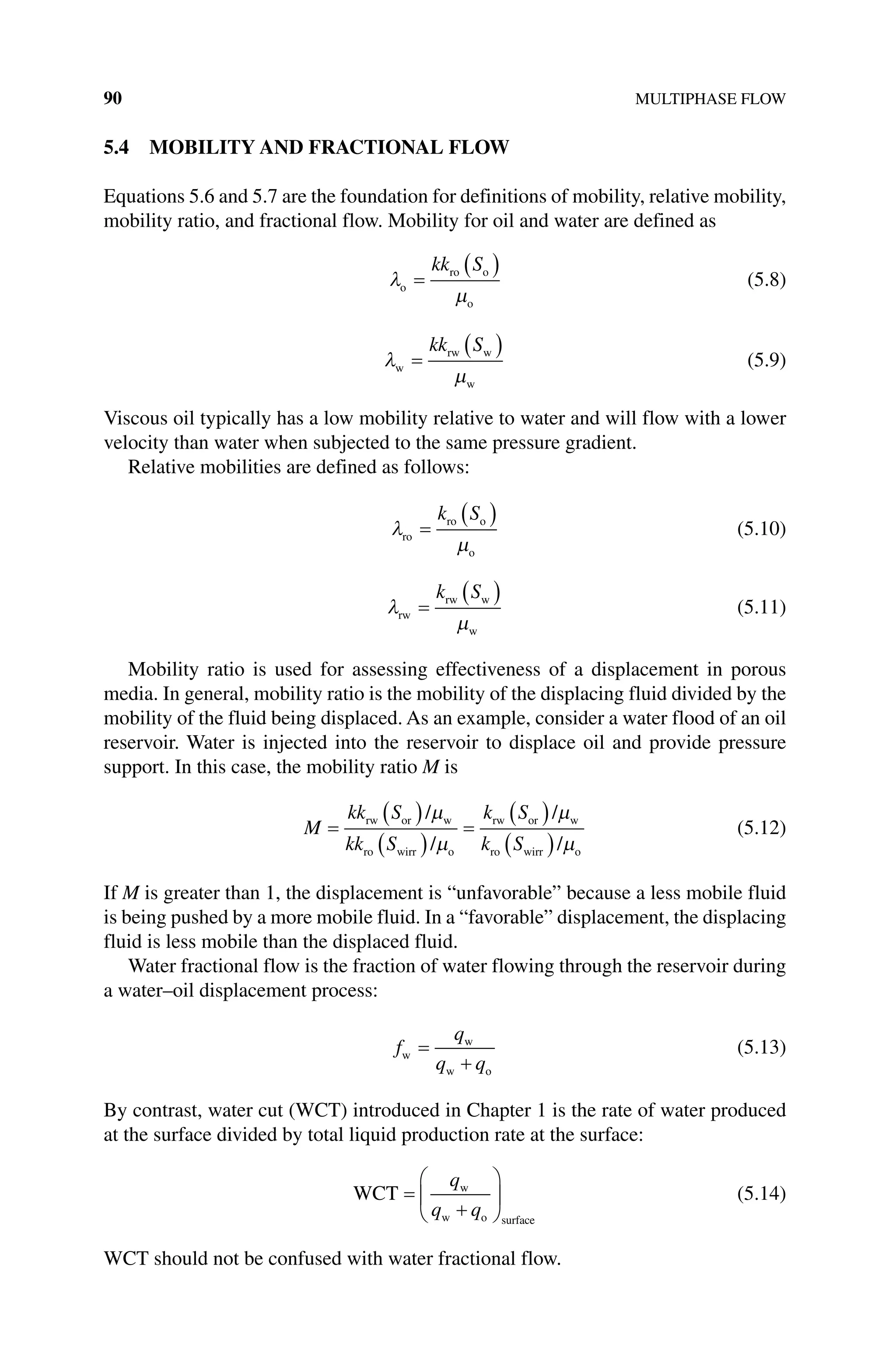
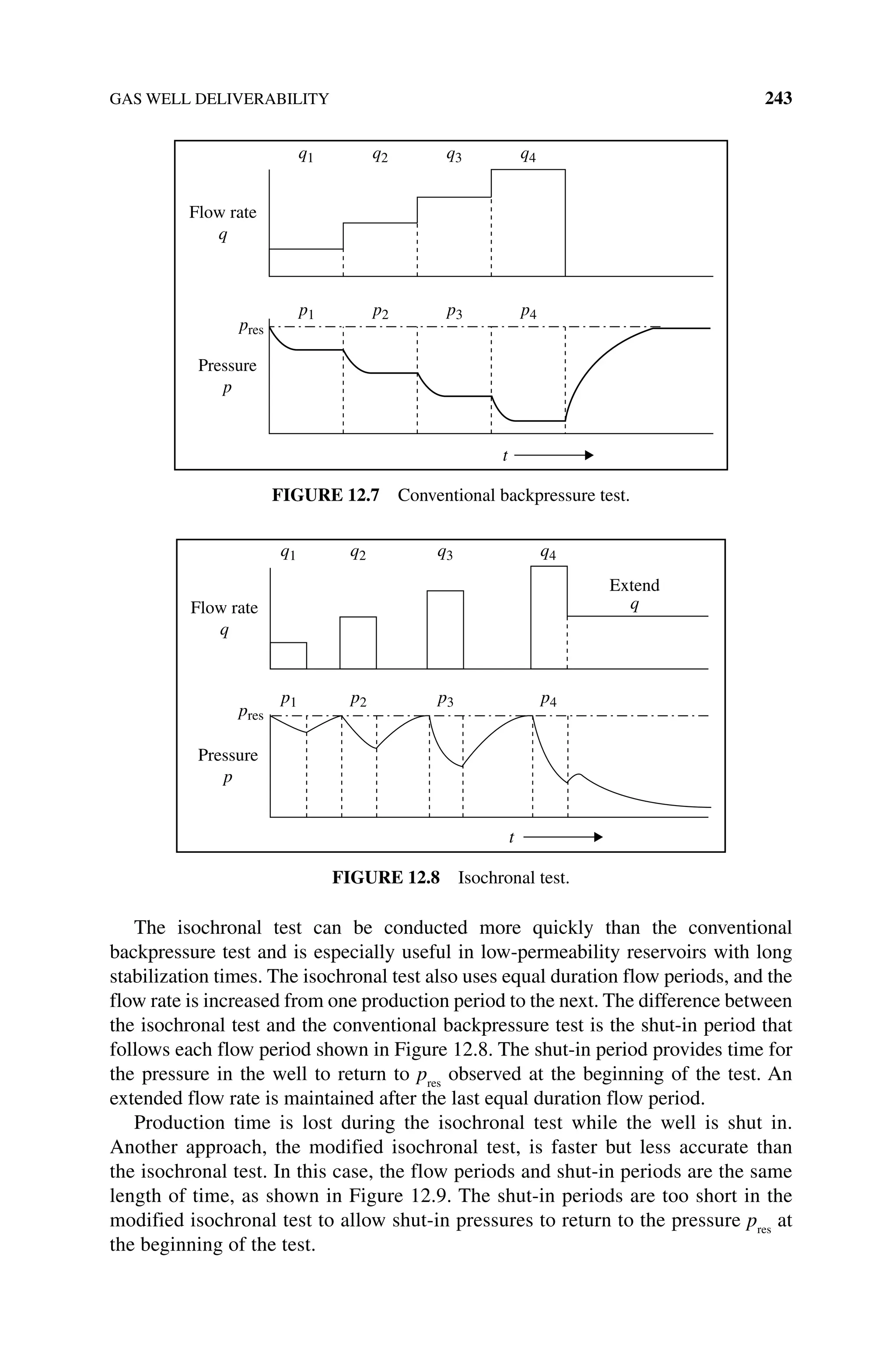
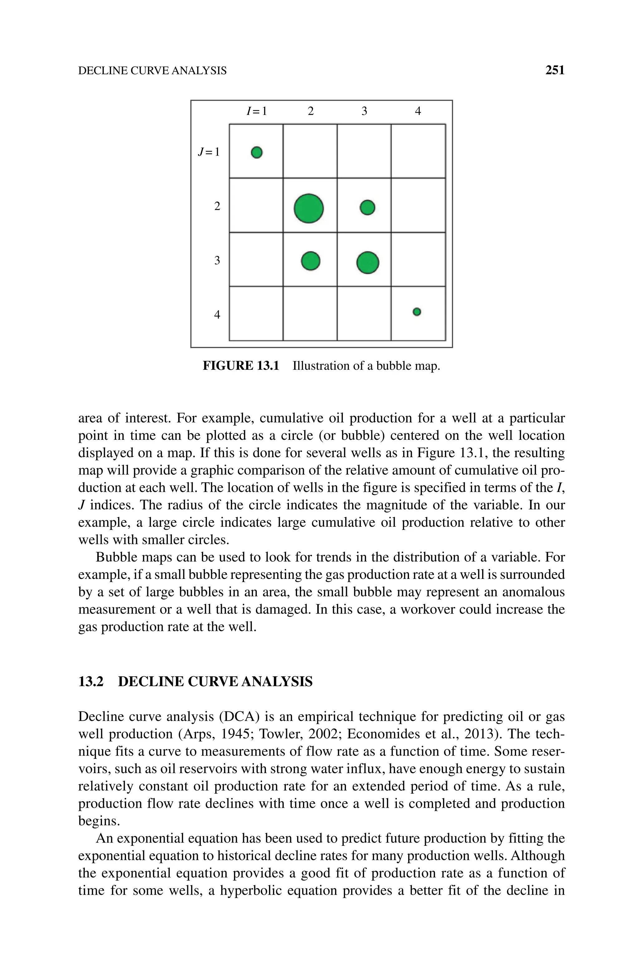
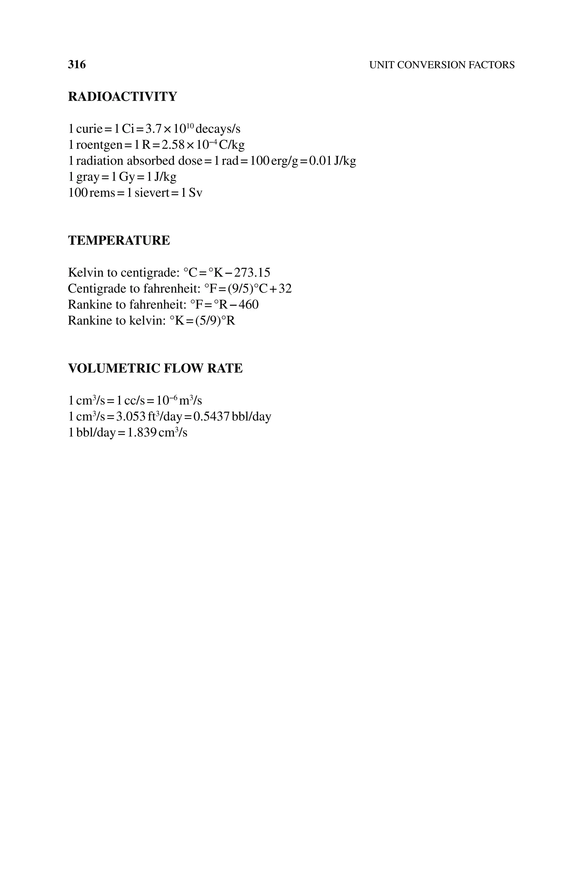
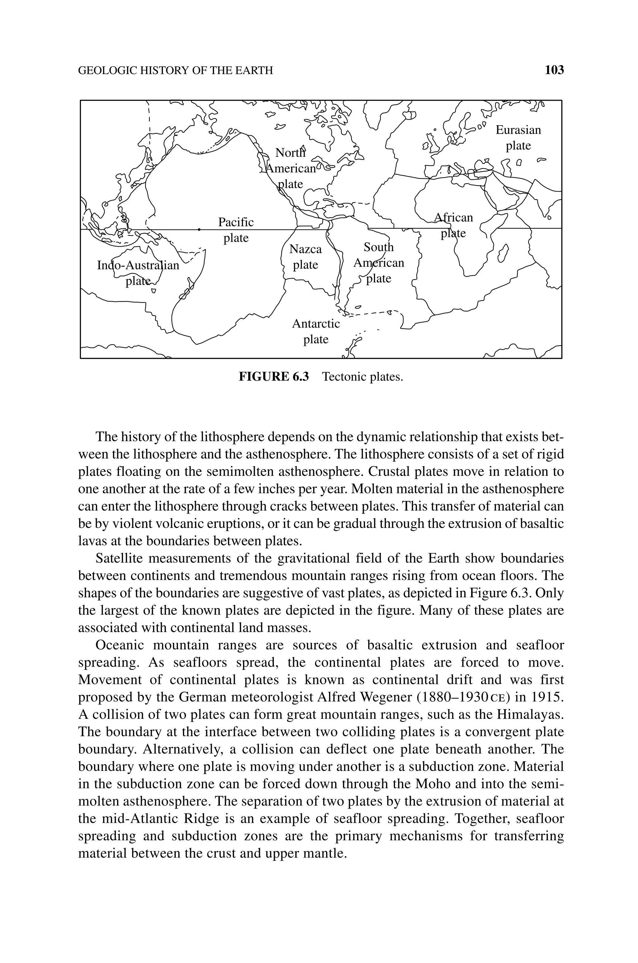
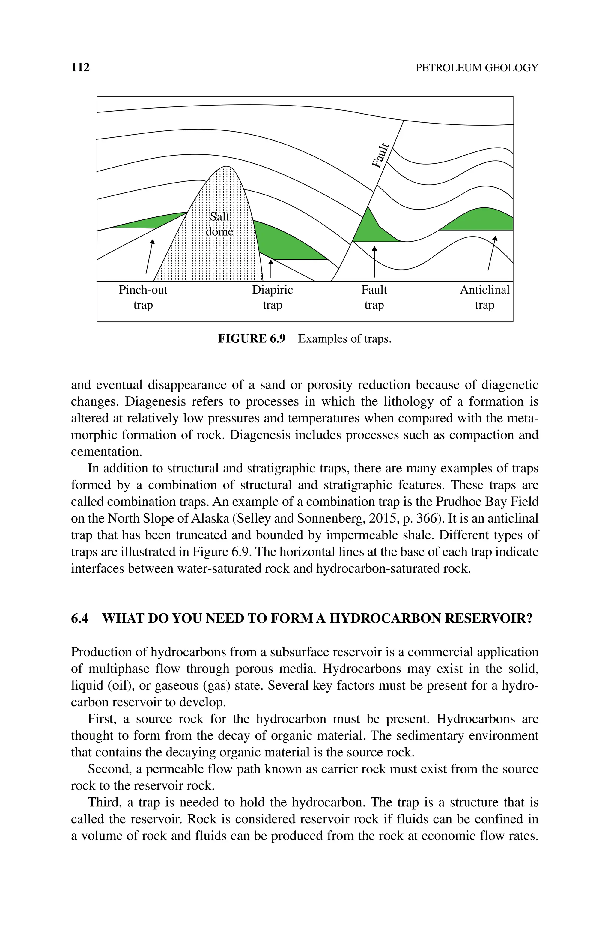
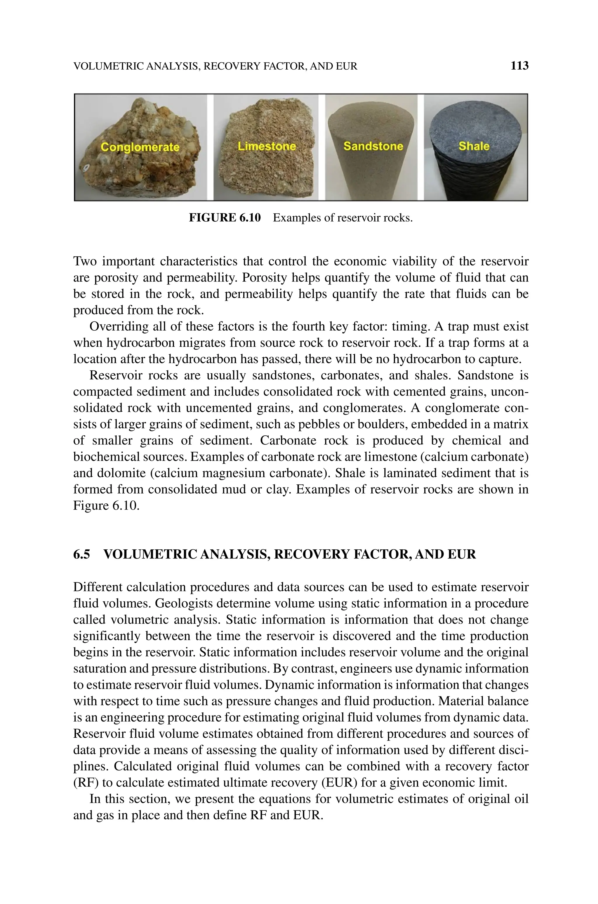
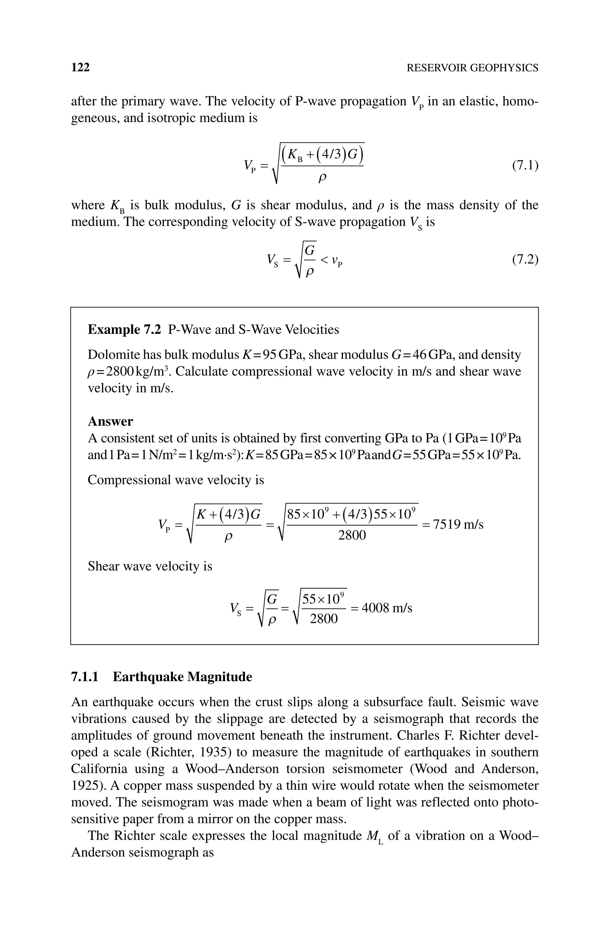
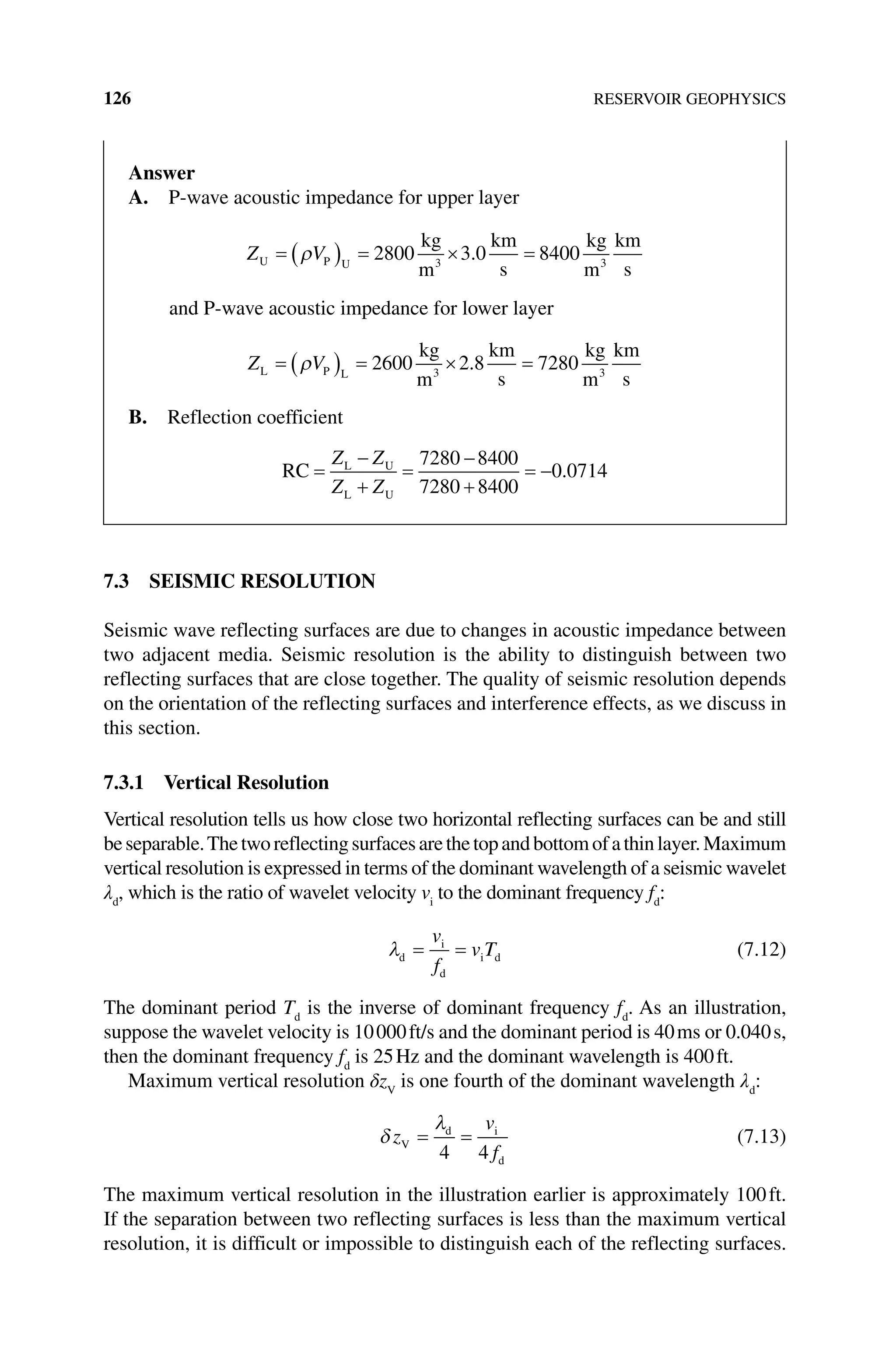
![ACTIVITIES 99
A. What is residual oil saturation (Sorw
)?
B. What is connate water saturation (Swc
)?
C. What is the relative permeability to oil at connate water saturation kro
(Swc
)?
D. What is the relative permeability to water at residual oil saturation krw
(Sorw
)?
E. Assume oil viscosity is 1.30 cp and water viscosity is 0.80 cp. Calculate
mobility ratio for water displacing oil in an oil–water system using the
data in the table and mobility ratio = λ λ µ
Displacing displaced rw orw w
/ / /
= ( )
( )
k S
ro wc o
( )
( / )
k S µ .
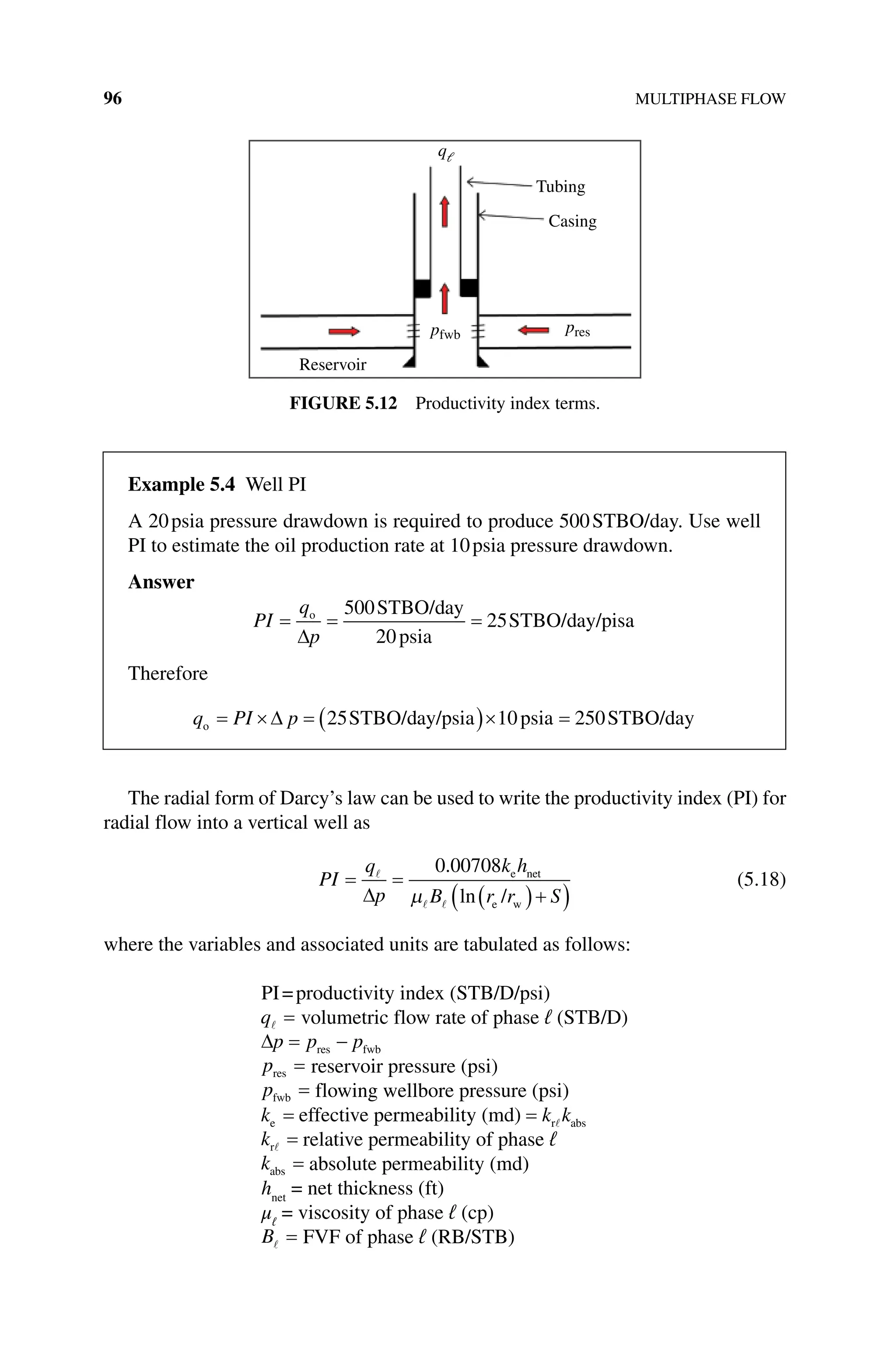
5.6 A well is producing oil in a field with 20‐acre well spacing. The oil has vis-
cosity 2.3cp and formation volume factor 1.25RB/STB. The net thickness of
the reservoir is 30ft and the effective permeability is 100md. The well radius is
4.5in. and the well has skin=0. What is the productivity index (PI) of the well
in STB/D/psi?
5.7 A.
Interfacial tension (IFT) σ can be estimated using the Weinaug–Katz vari-
ation of the Macleod–Sugden correlation:
σ σ
ρ ρ
1 4
1
1 4
1
/ /
= = −
= =
∑ ∑
i
N
i
i
N
i i
c c
P x
M
y
M
chi
L
L
V
V
where σ is the interfacial tension (dyne/cm), Pchi
is an empirical parameter
known as the parachor of component i [(dynes/cm)1/4
/(g/cm3
)], ML
is the
molecular weight of liquid phase, MV
is the molecular weight of vapor
phase, ρL
is the liquid phase density (g/cm3
), ρV
is the vapor phase density
(g/cm3
), xi
is the mole fraction of component i in liquid phase, and yi
is the
mole fraction of component i in vapor phase. The parachor of component
i can be estimated using the molecular weight Mi
of component i and the
empirical regression equation (Fanchi, 1990):
P Mi
chi = +
10 0 2 92
. .
This procedure works reasonably well for molecular weights ranging from
100 to 500. Estimate the parachor for octane. The molecular weight of
octane (C8
H18
) is approximately 8 12 18 1 114
* *
+ = , and the density of
octane in the liquid state is approximately 0.7g/cc.
B.
Estimate the contribution σi
of IFT for octane in a liquid mixture with
density 0.63g/cc and molecular weight 104. Assume there is no octane in
the vapor phase and the mole fraction of octane in the liquid phase is 0.9.](https://image.slidesharecdn.com/introductiontopetroleumengineeringbyjohnr-241125084112-ea228c08/75/Introduction-to-Petroleum-Engineering-by-John-R-Fanchi-pdf-113-2048.jpg)


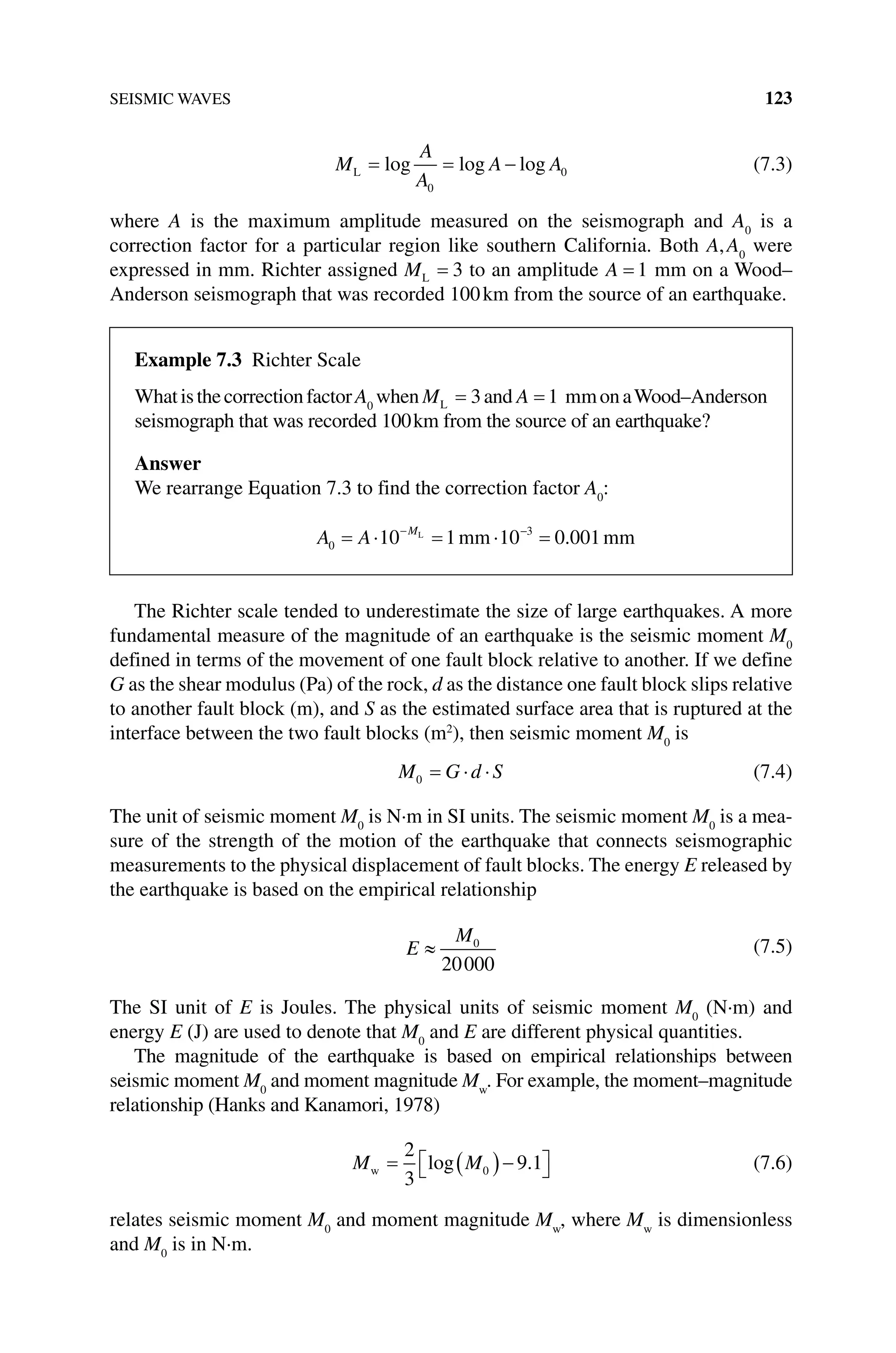
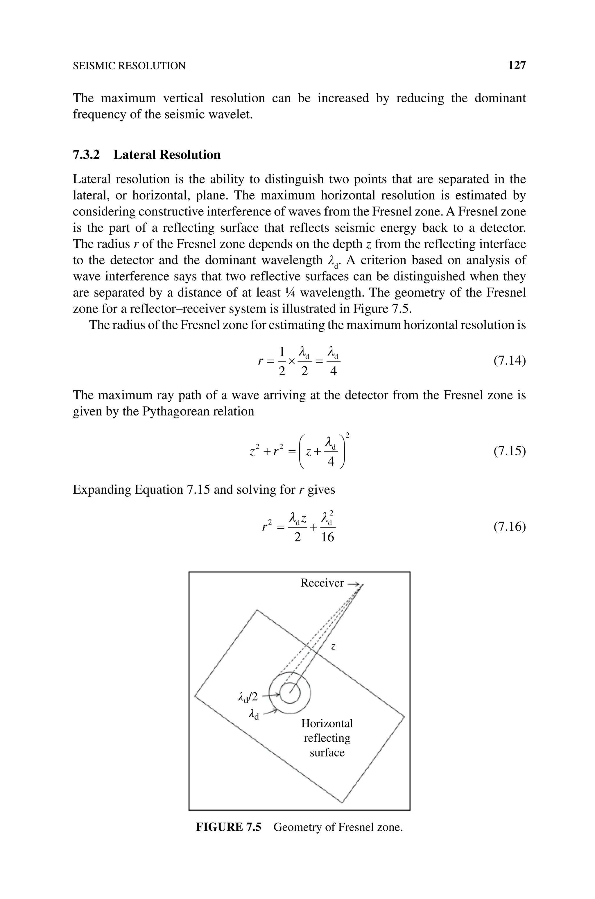


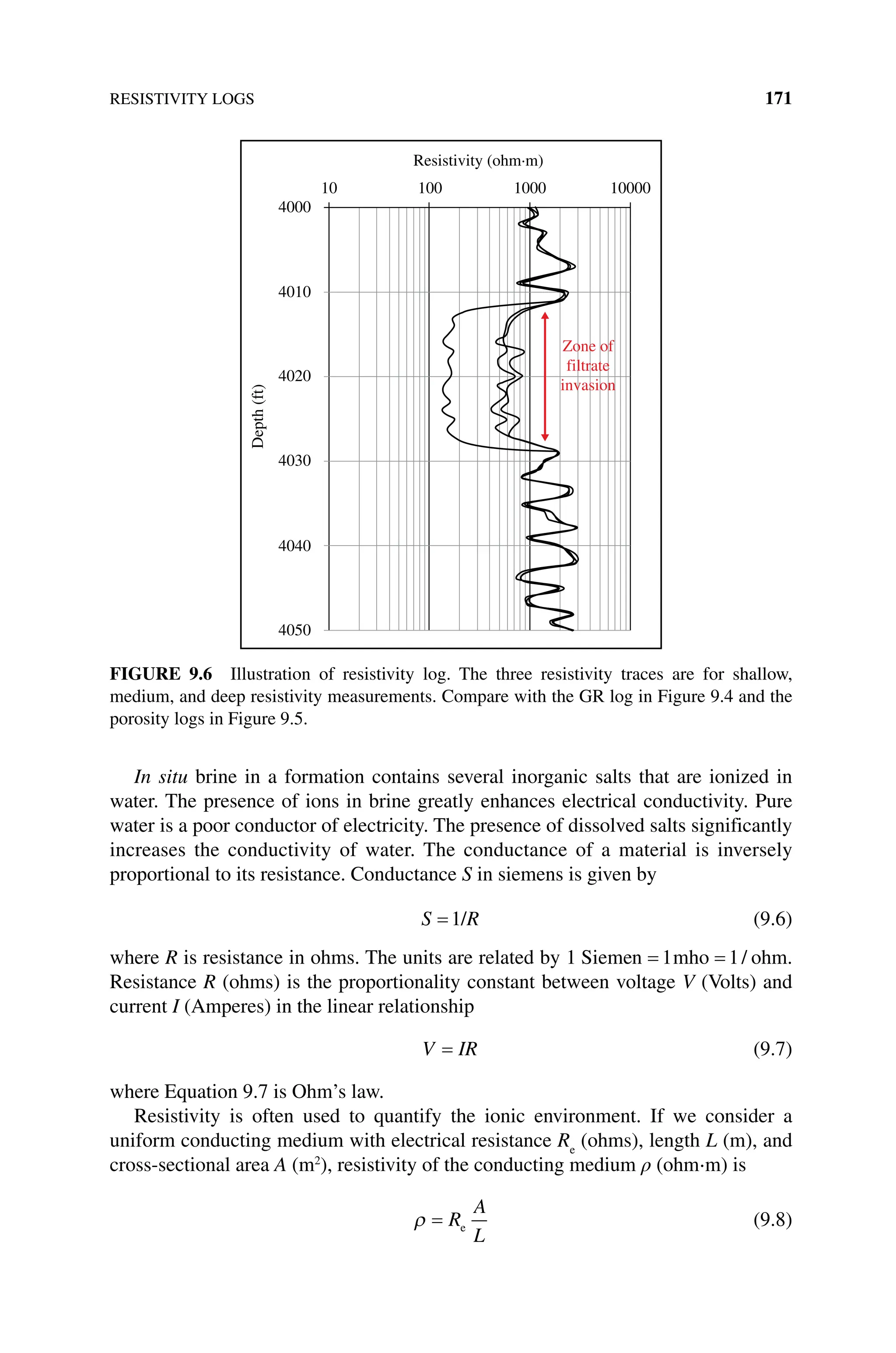
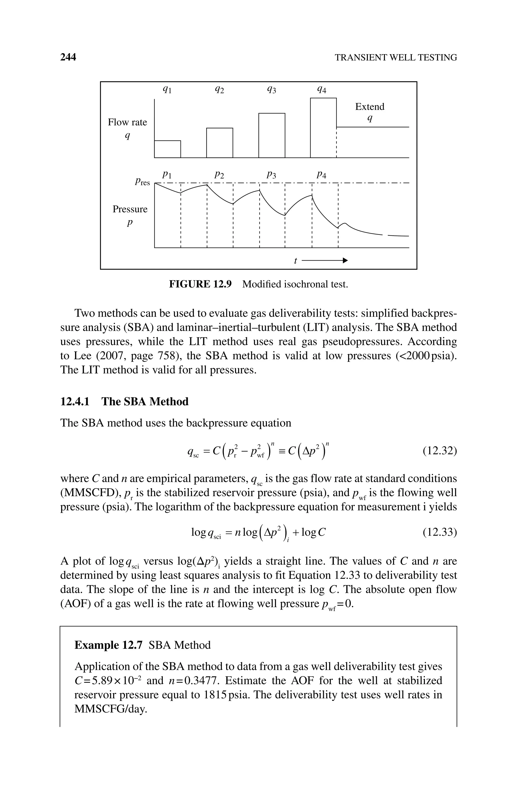
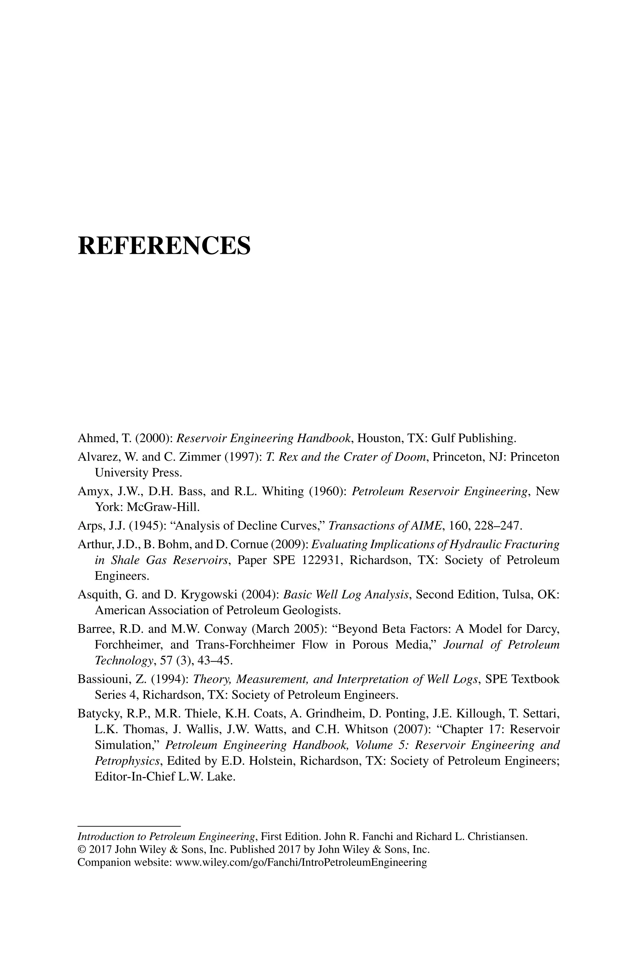
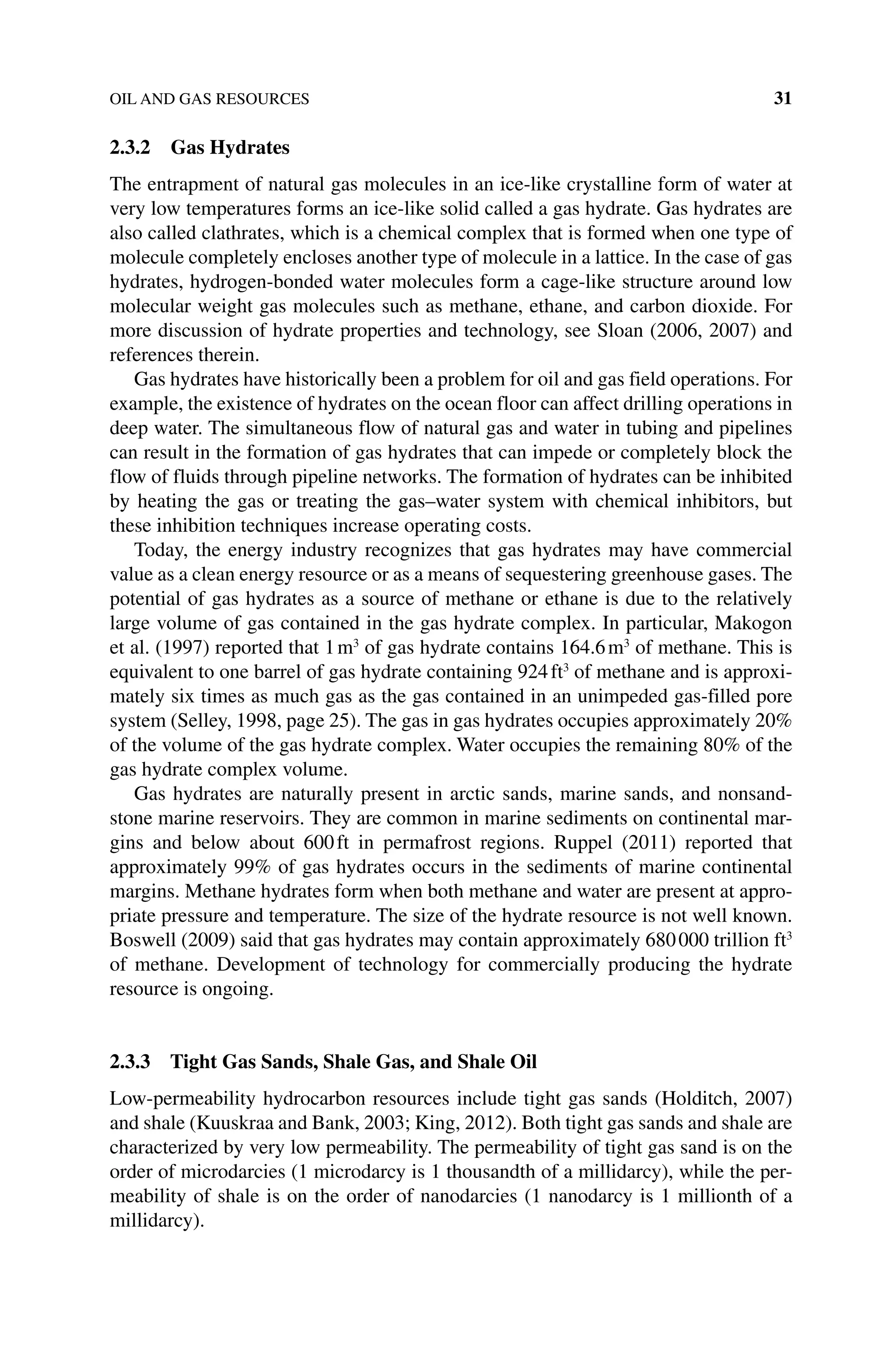
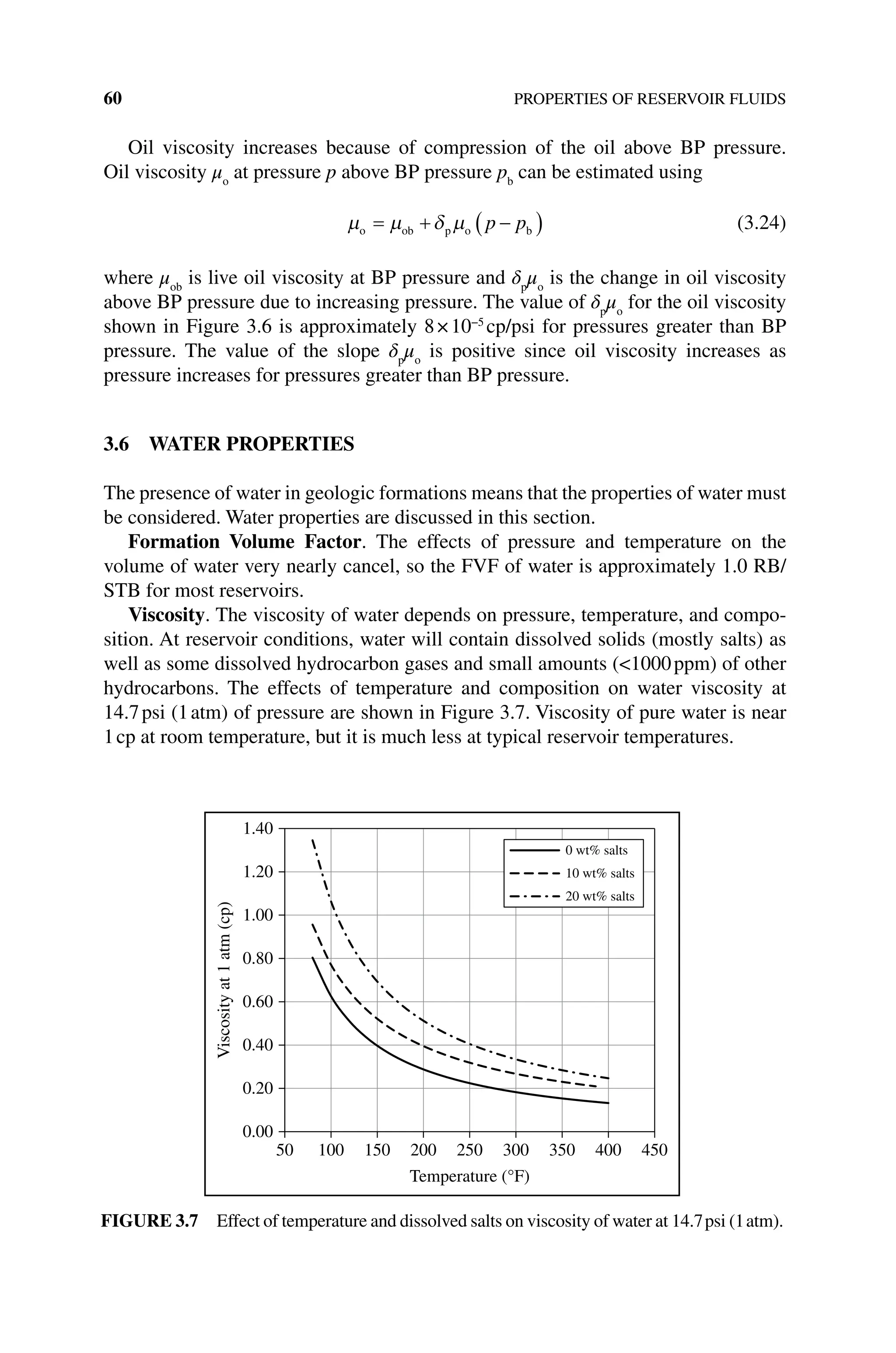
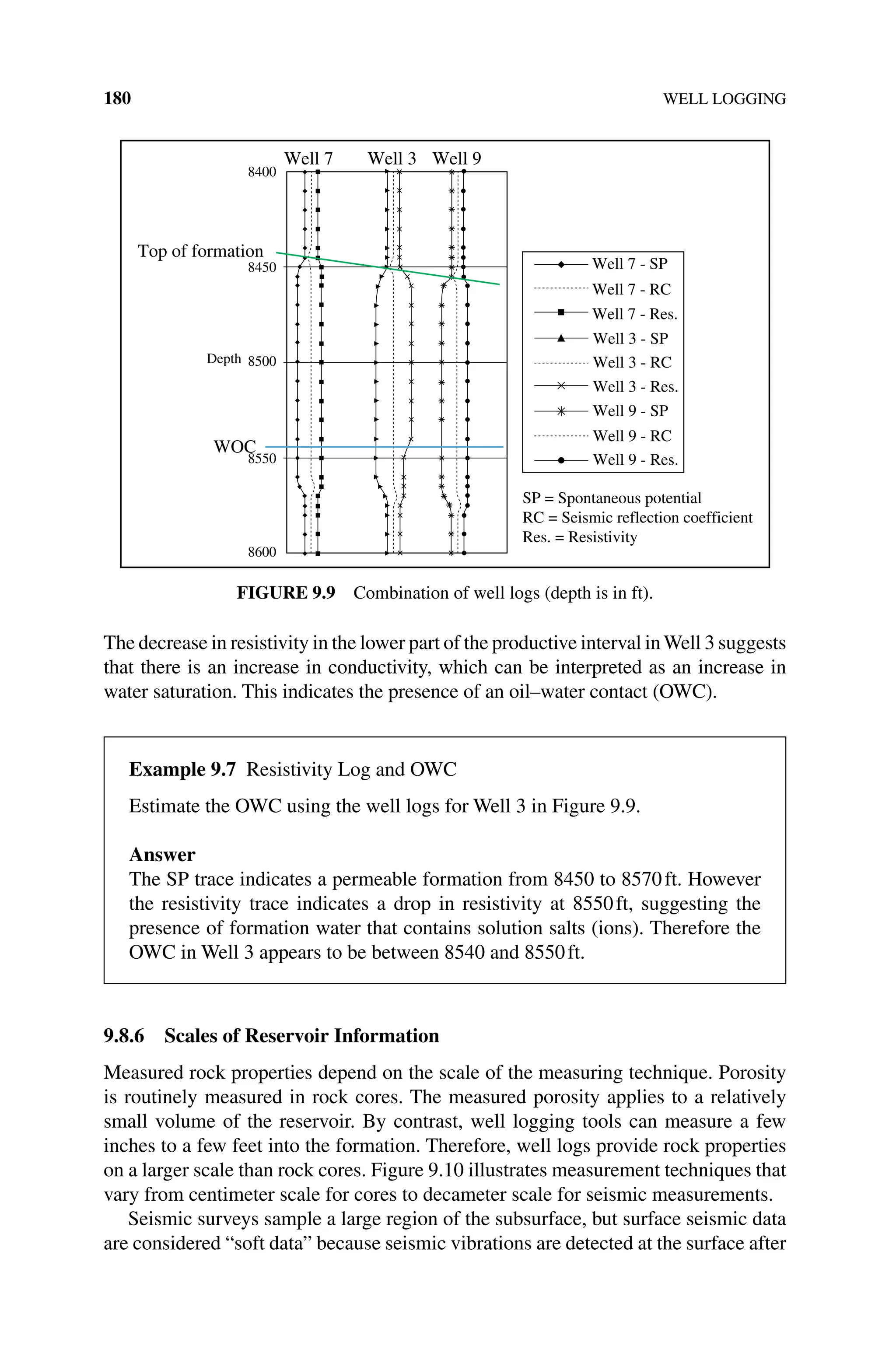
![172 WELL LOGGING
Resistivity ρ (ohm⋅m) is inversely proportional to electrical conductivity σ
(mho/m S/m
= ):
σ ρ
=1/ (9.9)
where1 1 1
S/m siemen/m mho/m
= = .
A high conductivity fluid has low resistivity. By contrast, a low‐conductivity fluid
like oil or gas would have high resistivity. A tool that can measure formation resis-
tivity indicates the type of the fluid that is present in the pore space. Resistivity in
a pore space containing hydrocarbon fluid will be greater than resistivity in the
same pore space containing brine.
The resistivity R0
of a porous material saturated with an ionic solution is equal to
the resistivity Rw
of the ionic solution times the formation resistivity factor F of the
porous material, thus
R FR
0 = w (9.10)
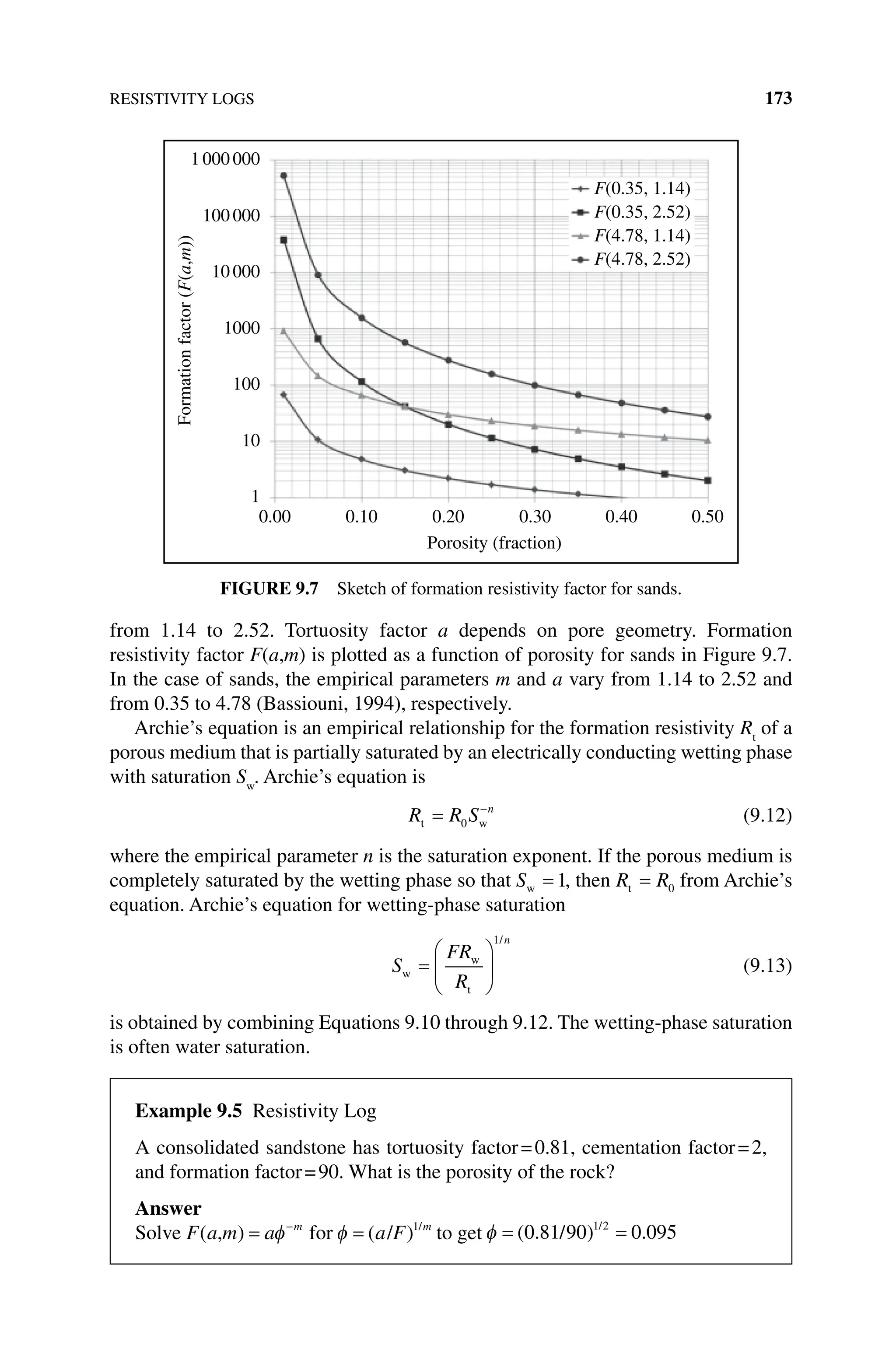
Formation resistivity factor F is sometimes referred to as formation factor. It can be
estimated from the empirical relationship
F a m a m
,
( ) = −
φ (9.11)
where ϕ is porosity, m is cementation exponent, and a is tortuosity factor. The cemen-
tation exponent m depends on the degree of consolidation of the rock and varies
Example 9.4 Ohm’s Law, Resistivity, and Conductivity
A. 0.006C of charge moves through a circuit in 0.1s. What is the current?
B. A 6V battery supports a current in a circuit of 0.06A. Use Ohm’s law to
calculate the resistance of the circuit.
C. Suppose the circuit has a length of 1m and a cross‐sectional area of
1.8m2
. What is the resistivity of the circuit?
D. What is the electrical conductivity of the circuit?
Answer:
A. Current [Ampere]
[Coulomb]
[Second]
C
s
A
= = =
0 006
0 1
0 06
.
.
.
B. Ohm’s law:Voltage V I R
( ) = × = ( )× ( )
current resistance A ohm orV IR
= .
Calculate / 6 V/ 6 A ohm
R V I
= = =
0 0 100
.
C. ρ = = = ⋅
R
A
L
e ohm
m
m
ohm m
100
1 8
1
180
2
.
D. σ
ρ
= =
⋅
= =
1 1
180
0 0056 5 6
ohm m
mho/m mmho/m
. . where mmho=
milli‐mho](https://image.slidesharecdn.com/introductiontopetroleumengineeringbyjohnr-241125084112-ea228c08/75/Introduction-to-Petroleum-Engineering-by-John-R-Fanchi-pdf-184-2048.jpg)


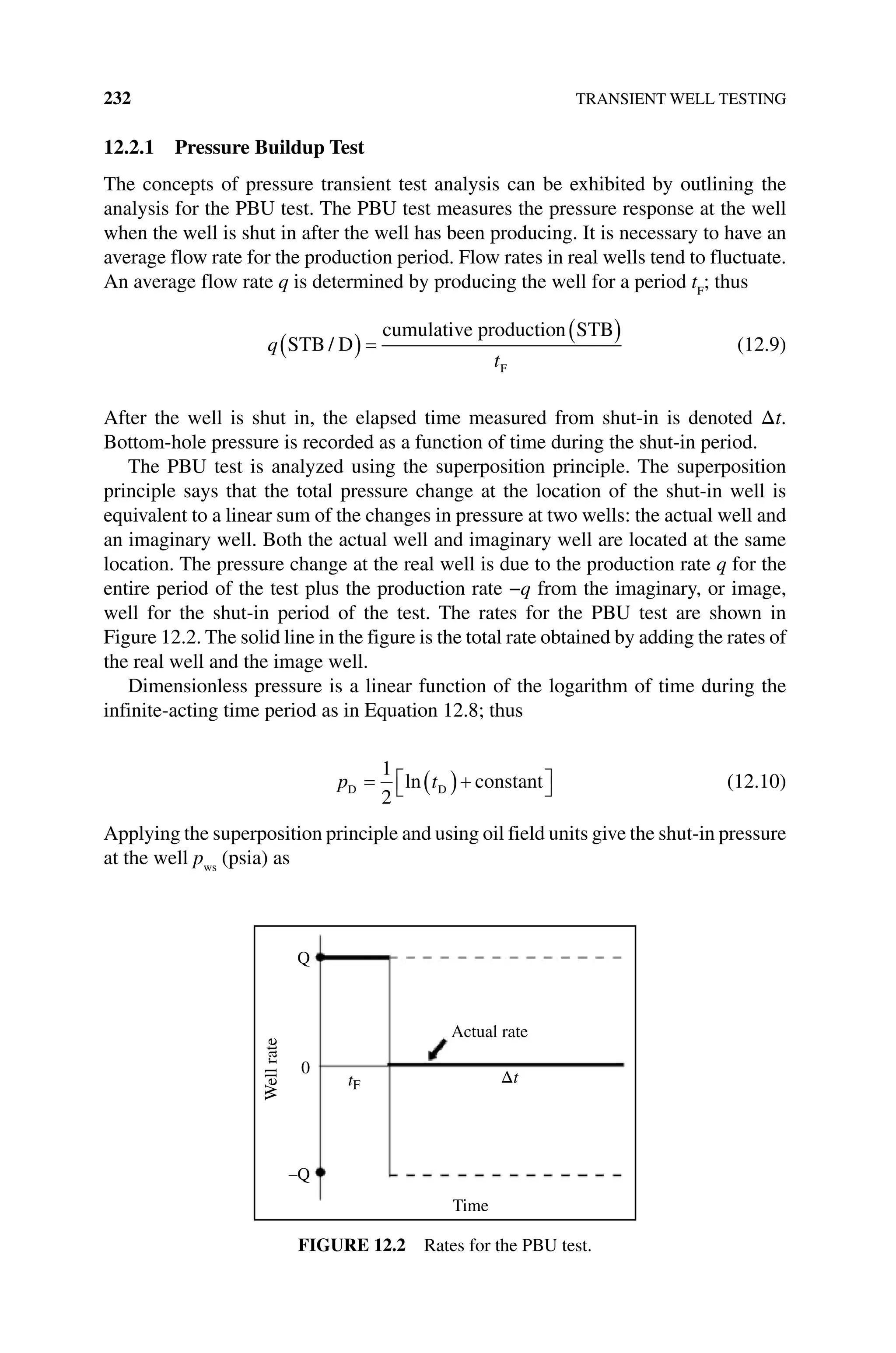
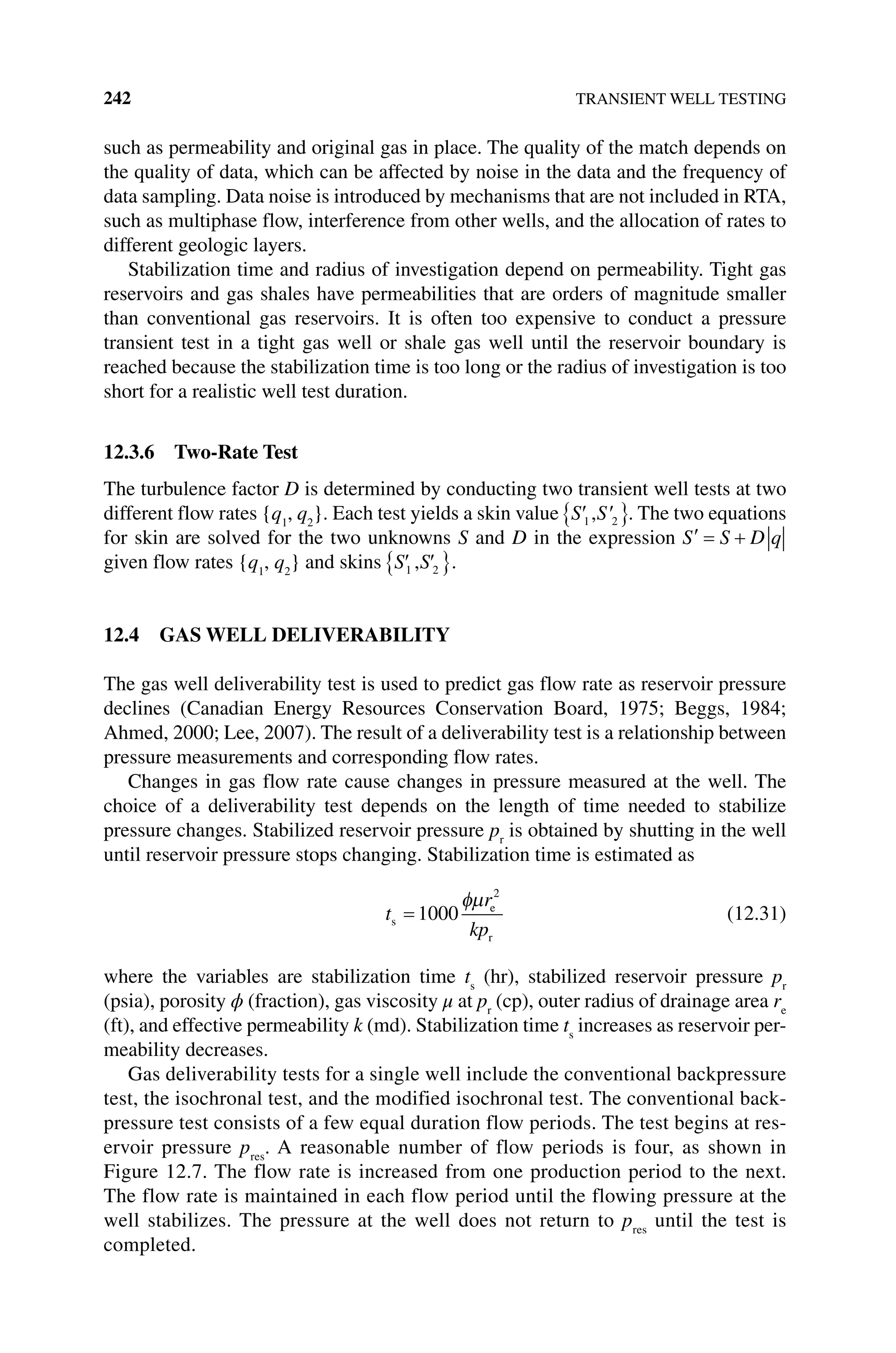
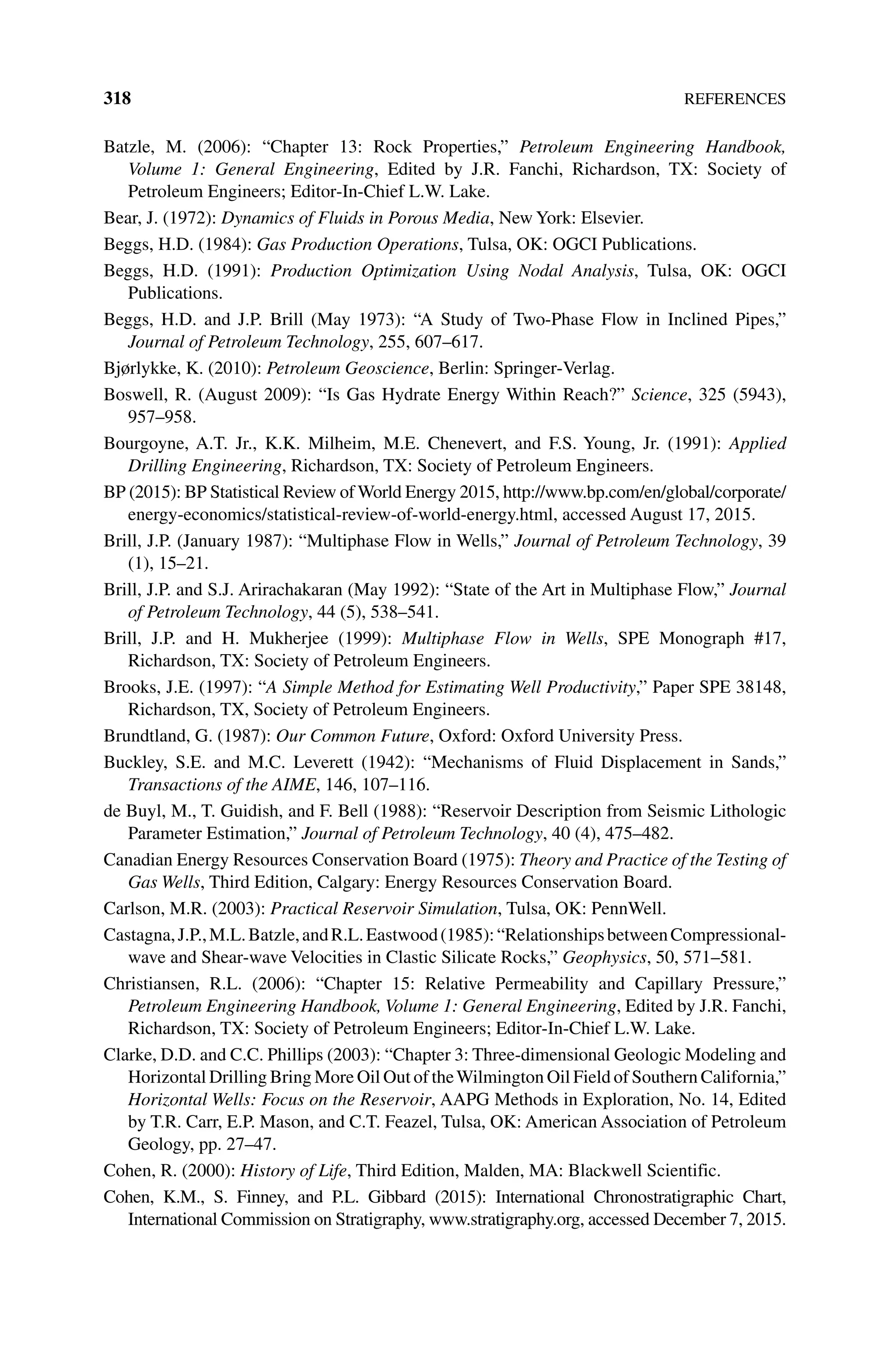
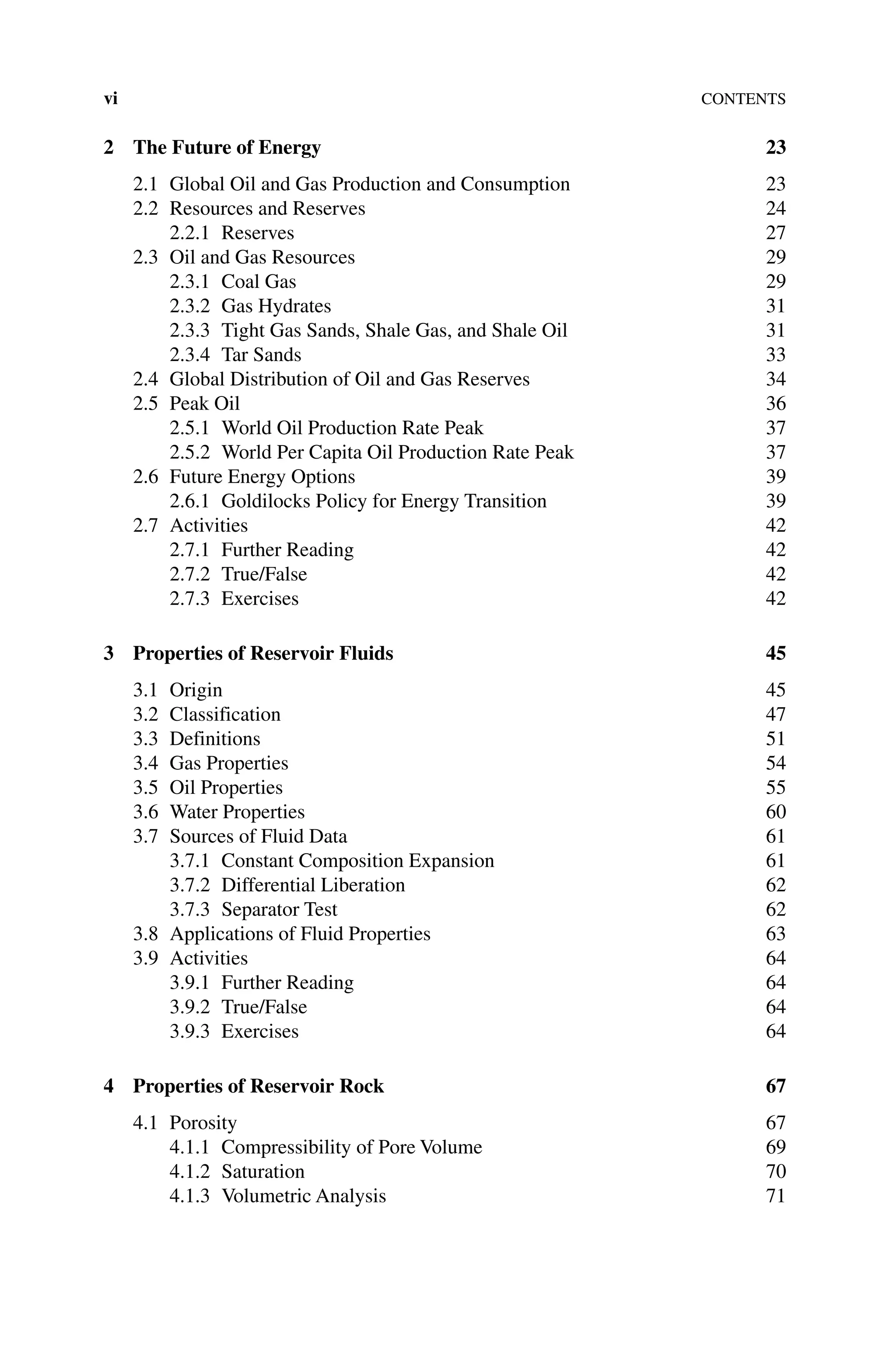
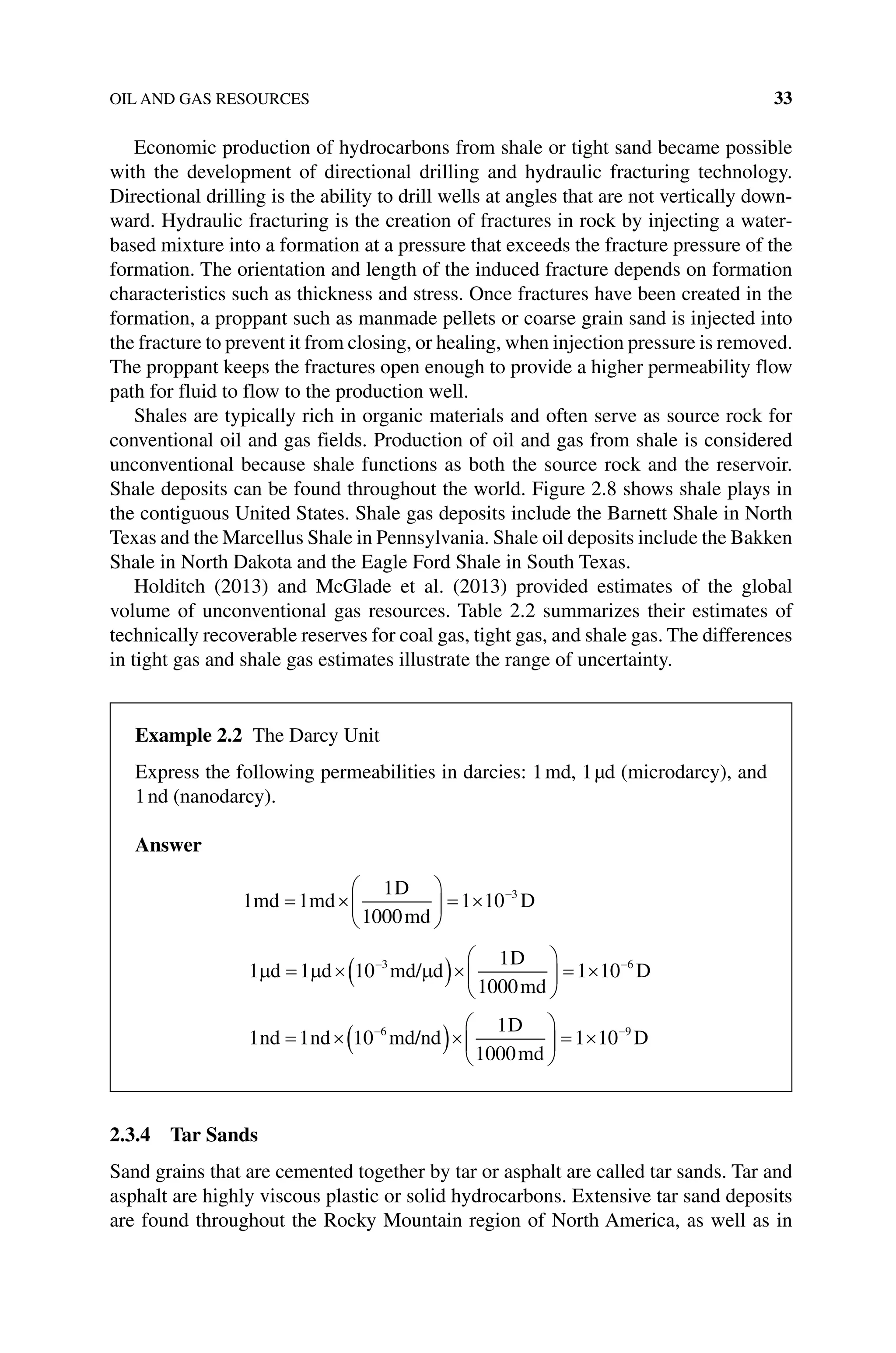
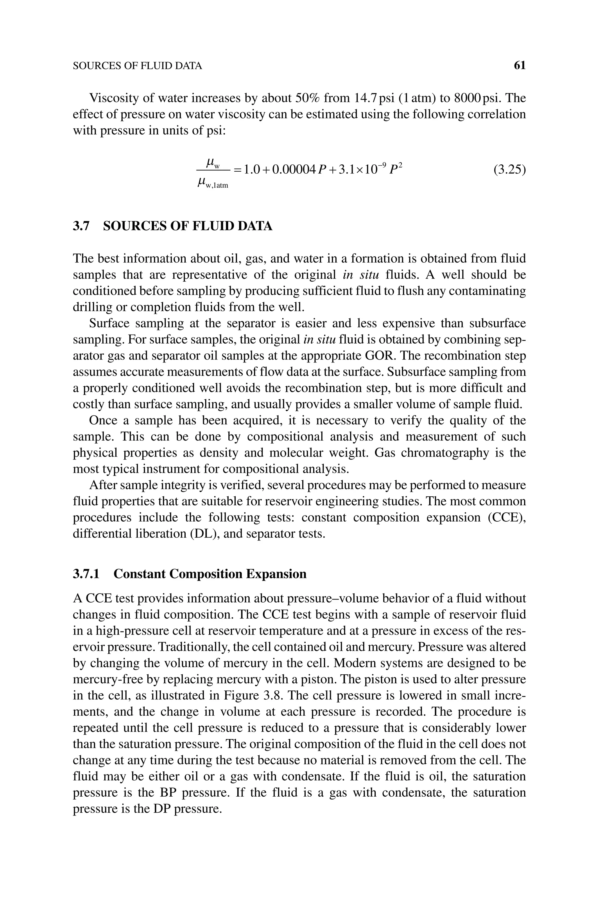
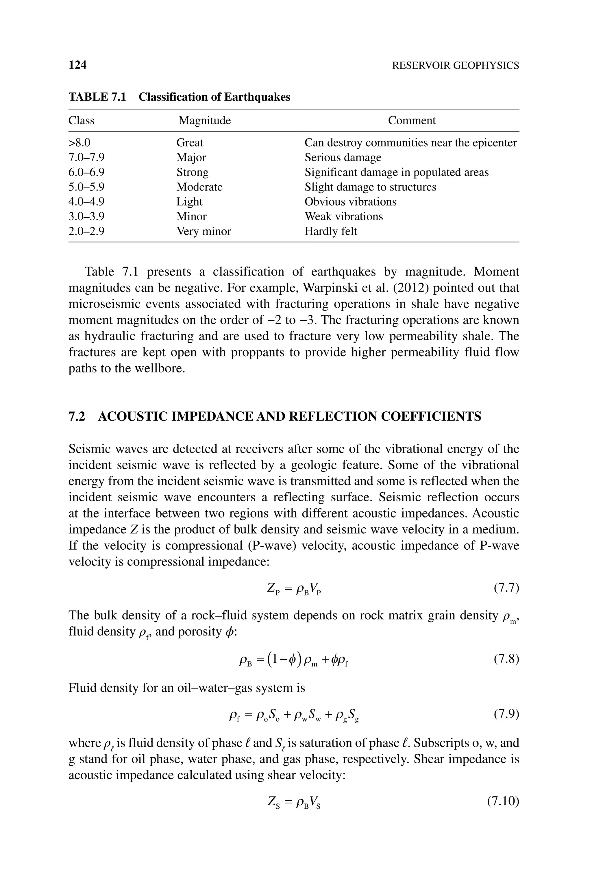
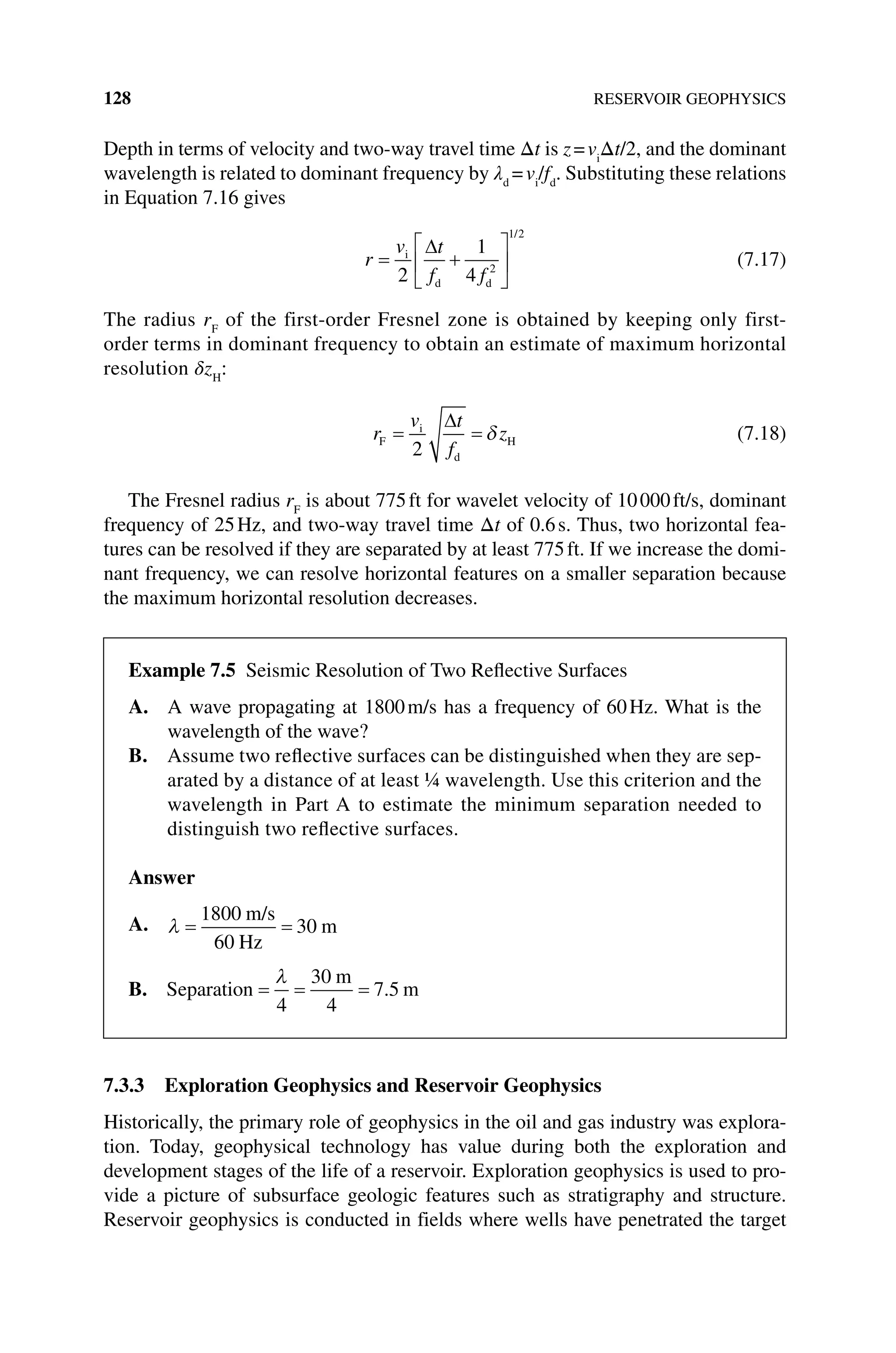
![OIL WELL PRESSURE TRANSIENT TESTING 233
p p
qB
kh
p t t p t
ws i D F D D D
141 2
. (12.11)
where pi
is the initial reservoir pressure (psia), q is the stabilized flow rate (STB/D),
B is the formation volume factor (RB/STB), μ is the viscosity (cp), k is the
permeability (md), and h is the net thickness (ft). The term p t t
D F D
( )
[ ] is
dimensionless pressure evaluated at dimensionless time [ ]
t t
F D, and the term
pD
(ΔtD
) is dimensionless pressure evaluated at dimensionless time ΔtD
. Dimensionless
pressure in Equation 12.11 is replaced by Equation 12.10 to obtain
p p m t
ws i H
log (12.12)
where tH
is the dimensionless Horner time:
t
t t
t
H
F
(12.13)
The hour is the unit of both times tF
,Δt to be consistent with the unit of time used in
the dimensionless time calculation. The variable m is given by
m
qB
kh
162 6
. (12.14)
The unit of m is psia per log cycle when pressure is in psia, q is stabilized flow rate
(STB/D), B is formation volume factor (RB/STB), μ is viscosity (cp), k is perme-
ability (md), and h is net thickness (ft). The concept of log cycle is clarified later.
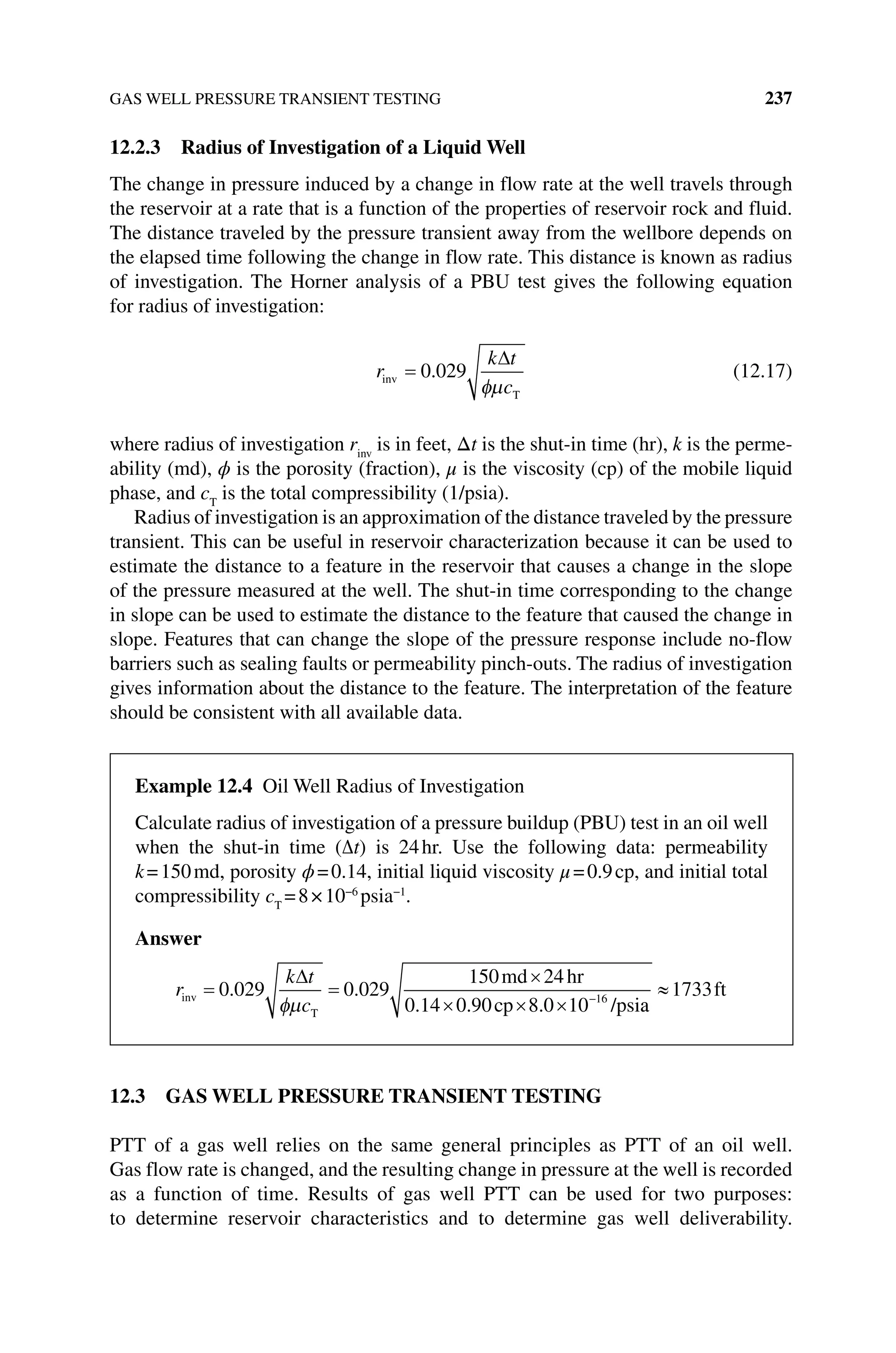
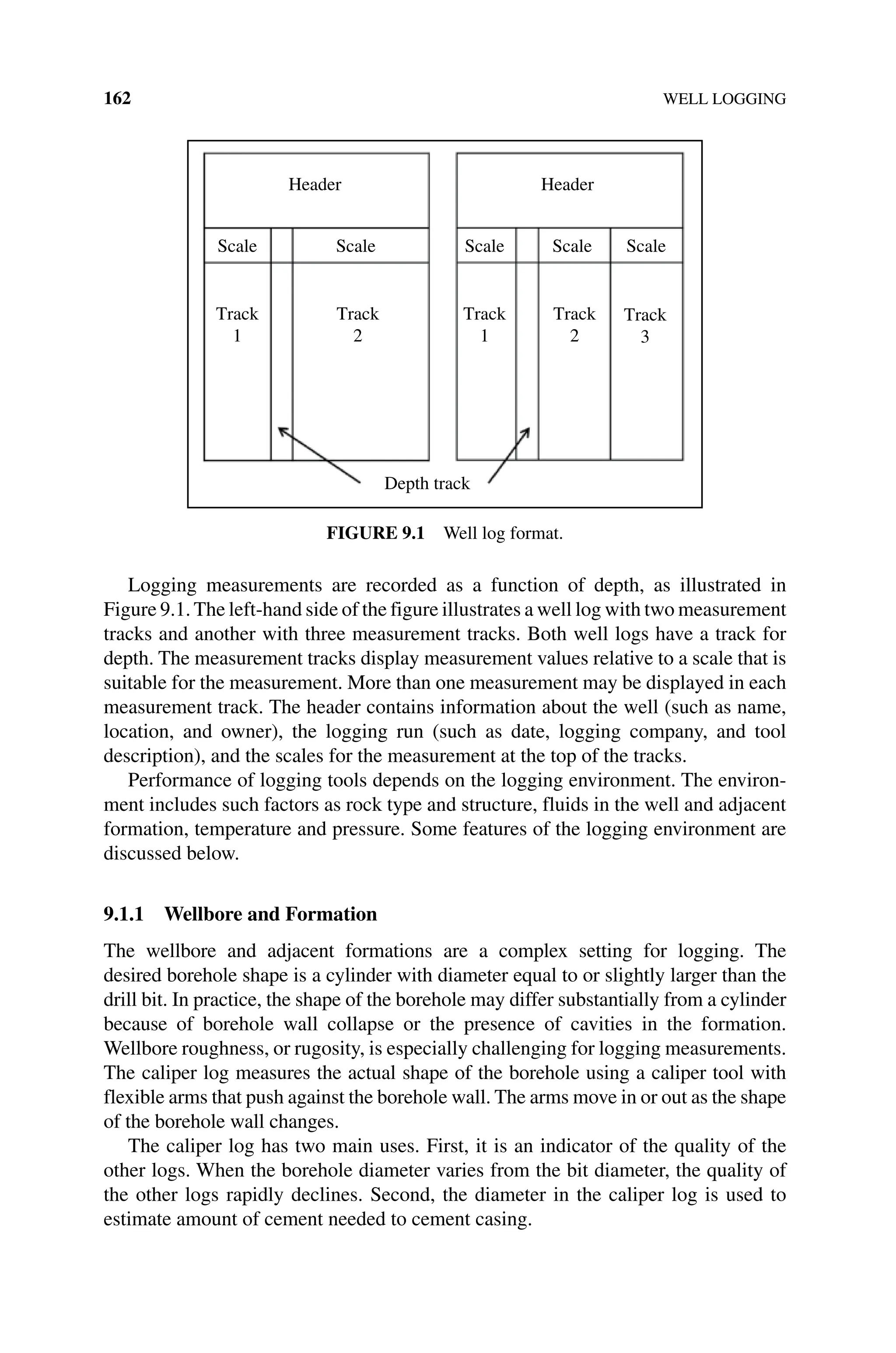
Equation 12.12 is the equation of a straight line if we plot pws
versus the logarithm
of Horner time on a semilogarithmic plot. The slope of the straight line is −m.
An example of the semilogarithmic plot for a PBU test is shown in Figure 12.3.
The plot is called a Horner plot.
The early time behavior of a Horner plot is displayed at large Horner times on
the right‐hand side of the plot. Later times correspond to smaller Horner times on
the left‐hand side of the plot. The wellbore storage effect appears as the rapid increase
of shut‐in pressure at early times in Figure 12.3 and does not end until Horner
time≈25. The infinite‐acting period appears as the straight line in the Horner time
Example 12.2 Horner Time
A well flows for 8hr with a stabilized rate before being shut in. Calculate
Horner time at a shut‐in time of 12hr.
Answer
The previous data gives Horner time t
t t
t
H
F 8 12
12
1 667
. .](https://image.slidesharecdn.com/introductiontopetroleumengineeringbyjohnr-241125084112-ea228c08/75/Introduction-to-Petroleum-Engineering-by-John-R-Fanchi-pdf-245-2048.jpg)