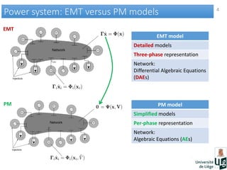
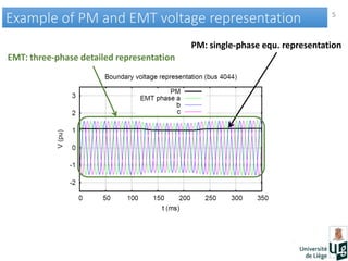
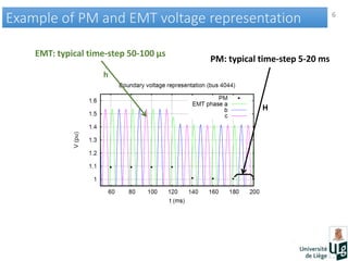
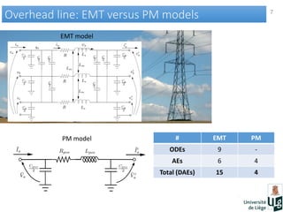
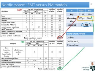
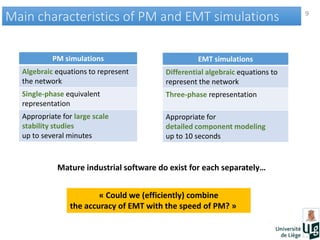
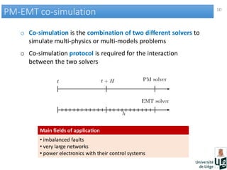
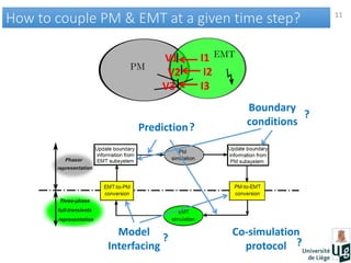
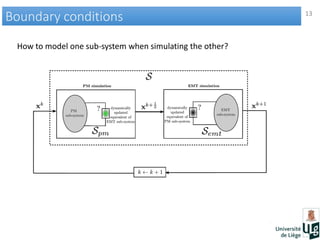
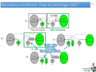
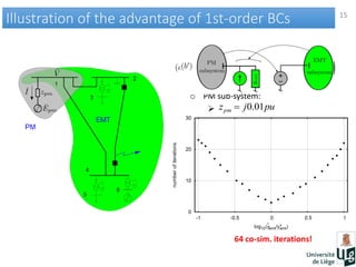
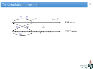
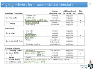
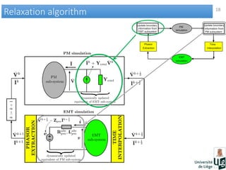
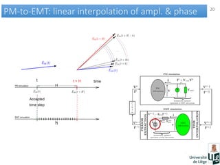
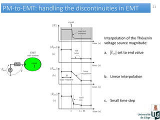
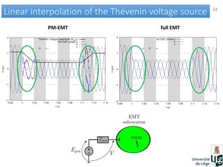
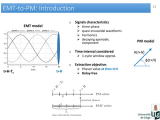
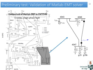
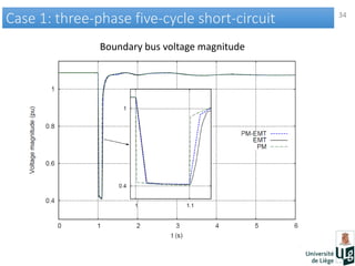
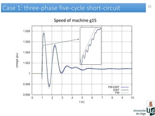
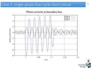
This document discusses co-simulation of electromagnetic transient (EMT) and phasor models for electric power system simulation. It presents methods for interfacing EMT and phasor models, including the use of dynamically updated Thevenin-Norton equivalents as boundary conditions and linear interpolation or least squares fitting for signal extraction. Several test cases demonstrate the approach on a 74-bus power system with single and multiple interface buses. The results show the co-simulation technique can accurately reproduce transient behaviors like oscillations and voltage fluctuations during faults.

1. Co-simulation of Electromagnetic Transients
and Phasor Models of Electric Power Systems
Frédéric Plumier
Department of Electrical Engineering and Computer Science
University of Liège
Liège, 29 January 2015

2. 2
General Structure of Power SystemsGeneral Structure of Power Systems
o Our economy is highly
dependent on Electrical Energy
o Complex, interconnected,
synchronous, systems
 Subject to external
aggressions
 Subject to volatility of
renewable sources
 Working closer to their
operating limit
o What if…
 fault occurs (lightning, …)?
 line switched off?
 generator outage?
o Modeling and simulations
needed!

3. 3
Dynamic phenomena in a Power SystemDynamic phenomena in a Power System
Power electronic controllers
EMT = ElectroMagnetic Transients
PM = Phasor-Mode

4. 4
Power system: EMT versus PM modelsPower system: EMT versus PM models
EMT model
Detailed models
Three-phase representation
Network:
Differential Algebraic Equations
(DAEs)
PM model
Simplified models
Per-phase representation
Network:
Algebraic Equations (AEs)
EMT
PM

5. 5
Example of PM and EMT voltage representationExample of PM and EMT voltage representation
PM: single-phase equ. representation
EMT: three-phase detailed representation

6. 6
Example of PM and EMT voltage representationExample of PM and EMT voltage representation
PM: typical time-step 5-20 ms
EMT: typical time-step 50-100 µs
H
h

7. 7
Overhead line: EMT versus PM modelsOverhead line: EMT versus PM models
# EMT PM
ODEs 9 -
AEs 6 4
Total (DAEs) 15 4
EMT model
PM model

8. 8
Nordic system: EMT versus PM modelsNordic system: EMT versus PM models
# EMT PM
Eqs 2287 609
time step
size
100µs 20ms
speedup ≈ 770
Nordic test system
74-bus,
102-branch,
23-machine.
EMT
PM
2 2

9. 9
Main characteristics of PM and EMT simulationsMain characteristics of PM and EMT simulations
PM simulations
Algebraic equations to represent
the network
Single-phase equivalent
representation
Appropriate for large scale
stability studies
up to several minutes
EMT simulations
Differential algebraic equations to
represent the network
Three-phase representation
Appropriate for
detailed component modeling
up to 10 seconds
Mature industrial software do exist for each separately…
« Could we (efficiently) combine
the accuracy of EMT with the speed of PM? »

10. 10
PM-EMT co-simulationPM-EMT co-simulation
o Co-simulation is the combination of two different solvers to
simulate multi-physics or multi-models problems
o Co-simulation protocol is required for the interaction
between the two solvers
Main fields of application
• imbalanced faults
• very large networks
• power electronics with their control systems

11. 11
How to couple PM & EMT at a given time step?How to couple PM & EMT at a given time step?
V1
V2
V3
I1
I2
I3
Boundary
conditions
Model
Interfacing
Co-simulation
protocol
Prediction?
?
? ?

12. 12
Outline of presentationOutline of presentation
o Coupling PM and EMT simulations
o Interfacing PM and EMT models
o Illustrative test results
o Summary of contributions

13. 13
Boundary conditionsBoundary conditions
How to model one sub-system when simulating the other?

14. 14
Boundary conditions: How to exchange info?Boundary conditions: How to exchange info?
Single-sided
First-order
Boundary Conditions
PM simulation EMT simulation
V = f(I)
V ≠ f(I)
Double-sided
First-order
Boundary Conditions

15. 15
Illustration of the advantage of 1st-order BCsIllustration of the advantage of 1st-order BCs
o PM sub-system:

o EMT sub-system
 56 diff. & 63 alg. states
pujzpm 01.0
64 co-sim. iterations!
3 co-sim.
iterations!

16. 16
Co-simulation protocolCo-simulation protocol

17. 17
Key ingredients for a successful co-simulationKey ingredients for a successful co-simulation

18. 18
Relaxation algorithmRelaxation algorithm

19. 19
Outline of presentationOutline of presentation
o Coupling PM and EMT simulations
o Interfacing PM and EMT models
o Illustrative test results
o Summary of contributions

20. 20
PM-to-EMT: linear interpolation of ampl. & phasePM-to-EMT: linear interpolation of ampl. & phase

21. 21
PM-to-EMT: handling the discontinuities in EMTPM-to-EMT: handling the discontinuities in EMT
Interpolation of the Thévenin
voltage source magnitude:
a. set to end value
b. Linear interpolation
c. Small time step
pmE

22. 22
Linear interpolation of the Thévenin voltage sourceLinear interpolation of the Thévenin voltage source
PM-EMT full EMT

23. 23
EMT-to-PM: IntroductionEMT-to-PM: Introduction
o Signals characteristics
 three-phase
 quasi-sinusoidal waveforms
 harmonics
 decaying aperiodic
component
o Time interval considered
 1-cycle window approx.
o Extraction objective:
 Phasor value at time t+H
 Delay-free
EMT model
PM model
t+Ht+H-Tx
A(t+H)
φ(t+H)

24. 24
EMT-to-PM: 1. least-squares curve-fittingEMT-to-PM: 1. least-squares curve-fitting
Aa(t+H), Ab(t+H), Ac(t+H)
φa(t+H), φb(t+H), φc(t+H)
Each of the
three phases
fitting one phase
Use the residuals as a measure
of the extraction quality

25. 25
EMT-to-PM: 1. least-squares curve-fittingEMT-to-PM: 1. least-squares curve-fitting
Choice of the curve f
f = f1: cosine waveform characterized
by a constant amplitude and a constant phase angle
f = f2: a quasi-cosine waveform,
whose amplitude and phase angle are linearly varying with time
f = f3: a quasi-cosine waveform of the type f2,
with the addition of a linearly varying DC component
f = f4: a quasi-cosine waveform of the type f2,
with the addition of an exponentially decaying aperiodic component
Literature
Proposed

26. 26
EMT-to-PM: 2. Projection on Synchronously
Rotating Axes (PSRA)
EMT-to-PM: 2. Projection on Synchronously
Rotating Axes (PSRA)

27. 27
EMT-to-PM: 2. Projection on Synchronously
Rotating Axes (PSRA) with a smoother
EMT-to-PM: 2. Projection on Synchronously
Rotating Axes (PSRA) with a smoother
Butterworth

28. 28
EMT-to-PM: Comparison of the TVEsEMT-to-PM: Comparison of the TVEs
Total Vector Error (TVE)

29. 29
EMT-to-PM: Problem at fault eliminationEMT-to-PM: Problem at fault elimination
o Time interval comprises two segments of
(quasi-)cosine waveforms with different
amplitudes and phase angles
o EMT-to-PM methods based on an
interval of time, not adapted
 Fourier transform
 Least-Squares fitting
o Combination of methods:
Least-squares and PSRA

30. 30
Outline of presentationOutline of presentation
o Coupling PM and EMT simulations
o Interfacing PM and EMT models
o Illustrative test results
o Summary of contributions

31. 31
Computing toolsComputing tools
PM solver: Ramses (ULg)
Implemented in FORTRAN 2003
Step size: 0.02s (1 cycle at 50 Hz)
EMT solver: Matlab-EMT (ULg)
Implemented in Matlab
State-space modeling
Step size: 100 µs
Validated through comparison with
EMTP-RV

32. 32
Preliminary test: Validation of Matlab-EMT solverPreliminary test: Validation of Matlab-EMT solver
5-cycles, single-phase fault
Comparison of Matlab-EMT to EMTP-RV

33. 33
Single boundary bus (4043)Single boundary bus (4043)
g15 & g15’ in EMT sub-system
thermal units,
600 MVA,
round rotor machines.
Test cases 1 & 2
Five-cycle short-circuit very near bus
4047,
Case 1: Three-phase fault,
Case 2: Single-phase fault.

34. 34
Case 1: three-phase five-cycle short-circuitCase 1: three-phase five-cycle short-circuit
Boundary bus voltage magnitude

35. 35
Case 1: three-phase five-cycle short-circuitCase 1: three-phase five-cycle short-circuit
Speed of machine g15

36. 36
Case 2: single-phase five-cycle short-circuitCase 2: single-phase five-cycle short-circuit
Phase currents at boundary bus

37. 37
Case 2: single-phase five-cycle short-circuitCase 2: single-phase five-cycle short-circuit
Relative error on the complex power flowing through the boundary bus

38. 38
Multiple boundary buses (4041, 4044, 4042)Multiple boundary buses (4041, 4044, 4042)
Test cases 3a, 3b, 4 & 5
Case 3: Three-phase fault at bus 1042,
a. marginally stable,
b. marginally unstable,
Case 4: Single-phase fault at bus 1042,
Case 5: Tripping g9 in PM sub-system.

39. 39
Case 3a: Three-phase fault, marginally stableCase 3a: Three-phase fault, marginally stable
o Voltages at interface buses
o Electromechanical
oscillations correctly
reproduced by PM-EMT
o PM shifted after 2s

40. 40
Case 3b: Three-phase fault, marginally unstableCase 3b: Three-phase fault, marginally unstable
Rotor speed of generator g6
Voltage magnitude at bus 4044

41. 41
Case 4: single-phase 10.5 cycle fault on bus 1042Case 4: single-phase 10.5 cycle fault on bus 1042

42. 42
Case 5: Tripping g9 in PM sub-systemCase 5: Tripping g9 in PM sub-system

43. 43
PM-EMT versus Static Thévenin equivalentPM-EMT versus Static Thévenin equivalent
Case 3a, 3b and 4: Relative error on
the complex power at bus 4044 when
using a static Thévenin equivalent.
Relative error on the complex power,
comparing PM-EMT to EMTP-RV
at boundary bus 4044, for test cases
involving multiple boundary buses.

44. 44
Convergence of the relax. process: Boundary Cond.Convergence of the relax. process: Boundary Cond.
Number of co-simulation iterations for various
boundary conditions and with 2nd order prediction
« Med » designates the median, and « Max » the
maximum value

45. 45
Convergence of the relax. process: PredictionConvergence of the relax. process: Prediction
Number of co-simulation iterations
for various predictions of the boundary variables
Reduction of
1 co-simulation iter!

46. 46
Single EMT eval. per time step for different BCsSingle EMT eval. per time step for different BCs
Case 3b: Relative error on complex power at bus 4044
when performing a single co-simulation iteration, with zero-order prediction.

47. 47
Single EMT error versus Fully converged errorSingle EMT error versus Fully converged error
Relative error on complex power at bus 4044
when performing a single co-simulation iteration.
Case 3a: Relative error on complex power
at bus 4044
when performing a single co-sim .iteration,
compared to the error
of the fully converged solution
with respect to the reference solution
(EMTP-RV).
Boundary conditions: type-(d)
Prediction: second order

48. 48
Outline of presentationOutline of presentation
o Coupling PM and EMT simulations
o Interfacing PM and EMT models
o Illustrative test results
o Summary of contributions

49. 49
Summary of contributionsSummary of contributions
Premise: With modern solvers, the EMT sub-system can be enlarged to the
extent that, at the interface with the PM sub-system, the three-phase
voltages and currents are almost sinusoidal and balanced
o Boundary conditions: Dynamically updated Thévenin – Norton equivalents
 Essential for good convergence
 Updating with frequency recommended
o Prediction of the boundary voltages and currents
o PM-to-EMT: linear interpolation of Thévenin voltage sources
o EMT-to-PM: Combination of
 Least-squares fitting of a quasi-cosine waveform including an
exponentially decaying aperiodic component
 Projection on Synchronously Rotating Axes (PSRA)
 Monitoring the residuals for switching between methods

50. 50
Summary of contributionsSummary of contributions
o Assessment of single co-simulation iteration accuracy
o Tests of marginally stable/unstable case
o Results presented on a 74-bus, 23-machine test system,
 split into one EMT and one PM sub-system with
• single interface bus,
• several interface buses.
 validated through comparison with EMTP-RV.

51. 51
Future extensions of the workFuture extensions of the work
o Using three-phase PM models for
 Intermediate layer,
 Whole PM sub-system,
o Identifying automatically the PM and the EMT sub-systems
suitable for a given event, in a given network,
o Switching back to PM-only simulation after the system has come
back to (three-phase balanced) steady state operation

52. 52
Future extensions of the workFuture extensions of the work
o Impact on the convergence of a larger number of boundary buses
to test if the convergence would be affected
o Using of a coarse EMT solver
 Prediction cannot be used when discrete event in EMT sub-system
 Serial protocol could be